Inverse Kinematics of Concentric Tube Steerable Needles

Abstract

Prior papers have introduced steerable needles composed of precurved concentric tubes. The curvature and extent of these needles can be controlled by the relative rotation and translation of the individual tubes. Under certain assumptions on the geometry and design of these needles, the forward kinematics problem can be solved in closed form by means of algebraic equations. The inverse kinematics problem, however, is not as straightforward owing to the nonlinear map between relative tube displacements and needle tip configuration as well as to the multiplicity of solutions as the number of tubes increases. This paper presents a general approach to solving the inverse kinematics problem using a pseudoinverse solution together with gradients of nullspace potential functions to enforce geometric and mechanical constraints.

I. Introduction

Needles are used to deliver drugs, implants and surgical tools to locations throughout the body. A fundamental limitation on the variety and complexity of procedures for which needles can be used is the extent to which a needle can be steered around delicate or bony structures during insertion as well as the capability to articulate the needle tip at the target site.

Recently, needles composed of precurved concentric tubes have been proposed as a technology which is capable of substantially increasing steerability and tip control in comparison to existing needles [10],[12],[13]. In this approach, the initial curvatures of the tubes interact to produce the mutual curvature along the length of the needle. Needle curvature can be controlled by rotating and translating the tubes with respect to each other. Fig. 1 depicts an example comprised of four tubes.

Figure 1.

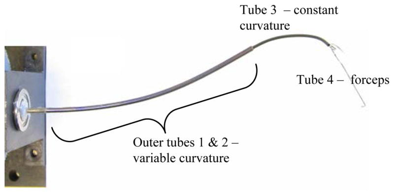
Four-tube steerable needle with forceps grasping a suture needle.

While closed-form inverse kinematic equations have been derived for several simple needle designs [10], a general approach to inverse kinematics is needed which can be employed for both closed-loop control and surgical planning. The method must be computationally efficient to be useful for control and should also, in the case of kinematic redundancy, enable exploration of the self motion manifold to compare alternative paths to surgical targets.

This is a difficult problem since computation of concentric-tube needle curvature is a 3D beam bending problem. Solving problems of this type typically requires numerical integration along the length of the beam to solve a two-point boundary value problem [1]. Such a model is cumbersome to implement in a surgical planning system let alone for real-time control. Alternatively, as introduced in [10], an approximate algebraic model for beam curvature can be adopted. While this model makes certain assumptions, such as negligibility of external forces on the shape of the needle and torsional rigidity of the individual tubes, it substantially reduces the computational complexity of the kinematics. Using this model, tubes of initial piecewise constant curvature combine to form steerable needles of piecewise constant curvature [10].

This paper presents a generalized inverse Jacobian approach for efficiently solving the inverse kinematics problem for concentric tube needles. This approach also facilitates mapping of the self-motion manifold as well as the inclusion of constraints on tube length and curvature. While the algebraic curvature model of [10] is used here, the approach applies to any algebraic curvature model which results in a needle of piecewise constant curvature. Such a shape is advantageous for a concentric tube needle, since it can be inserted into tissue in a telescoping fashion while applying minimum off-axis forces to the tissue.

Generalized inverse Jacobian solutions to the kinematics problem are widely reported in the literature for robots comprised of links and joints [3],[5],[6]. Steerable needles, however, belong to the class of continuum robots which lack discrete links and joints [9]. The kinematics of these systems have been addressed in [2],[4],[11].

In contrast to hyper-redundant manipulators, the number of kinematic variables of a steerable needle (relative tube rotations and translations) is modest. Thus, while the coordinate frames employed here have some similarity to the backbone reference frames of [2], the kinematic map is most easily expressed in terms of shape functions specific to the component tubes (i.e., piecewise constant curvature) rather than a more general modal mapping. In approach, this paper is closest to [4] which derives the kinematic map for a multi-section continuum robot in which the curvature and length of each section is determined by the length of three cables equally spaced around the trunk. The present work differs from [4] in several respects. First, the kinematic inputs are the relative rotations and translations of the tubes. Second, the curvature of each needle section depends on all tubes within that section and the number of sections can vary as tubes are extended and retracted. Third, constraints on tube length and curvature exist which can be directly incorporated in the inverse solution.

In the next section, the forward kinematic map between the tube variables and needle tip frame is derived as the product of three mappings. Section III develops the inverse solution to these three maps. The subsequent sections provide examples inverse kinematic solutions for several needle designs as well as conclusions.

II. Forward Kinematic Modeling

Using the methodology proposed in [10], needles can be designed and described according to the relative bending stiffness between sets of tubes. Limiting cases correspond to when the bending stiffness ratio of a pair of tubes is either close to one (balanced stiffness) or very large (dominating stiffness). In this approach, a needle design can be described in terms of the stiffness ratios of its tubes starting from the outermost tube and proceeding to the innermost. For example, the design of Fig. 1 can be described as (1) balanced stiffness I₁/I₂ ≈ 1, (2) dominating stiffness (I₁ + I₂) ≫ (I₃ + I₄) and (3) dominating stiffness, I₃ ≫ I₄. Note that tube 4 has zero initial curvature. When the tubes are extended in telescoping fashion, this ordering also describes the ordering of controllable sections from the proximal to the distal end.

When balanced stiffness tubes are rotated with respect to each other, their combined curvature varies. This is the case for the outer pair of tubes in Fig. 1. As the relative rotation angle between these tubes is changed, their curvature varies from zero (straight) to a maximum value. If, as shown in Fig. 1, additional tubes are contained inside this pair, which are very flexible in comparison to the outer pair, the shape of the inner tubes conforms to that of the outer pair. If these inner tubes are extended beyond the end of the outer tubes, however, they relax to their own curvature.

The kinematic input variables (θ, l) for each tube consist of its rotation angle, θ, and extension length, l. It is assumed here that any balanced stiffness tube pairs in a design are included for curvature control over their mutual length and so their extension lengths are constrained to be equal. For a needle comprised of n tubes with p balanced pairs, the kinematic input variables can arranged in m = n − p groups of either (θ, l)_i or (θ₁, θ₂, l)_i. The latter applies for balanced stiffness pairs.

The kinematic mapping from tube variables to needle tip frame is diagrammed in Figure 2 as a product of three mappings. The first mapping converts the tube kinematic variables to m corresponding input curves of curvature κ̂_i(s) = [κ̂_x(s) κ̂_y(s)]_i and extension length, l_i. These m curves are of piecewise constant curvature. The second mapping converts the input curves to the actual arcs of the needle, (κ_x, κ_y, s)_j, j = 1, …, n, where the number of arcs, n, is the total number of constant curvature segments for all the tubes combined. These two mappings are considered separately because the designs of the individual tubes are most easily described in the input curve space. This proves useful when computing the inverse kinematics.

Figure 2.

Kinematic mappings.

The third mapping determines the needle tip coordinate frame, W^{W (0)}(l _m), with respect to the needle base frame from the sequence of needle arcs as previously described in [10].

A. Mapping Tube Parameters to Input Curves

Balanced stiffness tube pairs require use of a curvature model in this step. The model from [10] will be used here. For a set of p tubes, the resultant curvature is

$${\kappa }_f={\left(\sum _{i=1}^p{K}_i\right)}^{-1}\sum _{i=1}^p{K}_i{\overline{\kappa }}_i,$$ (1)

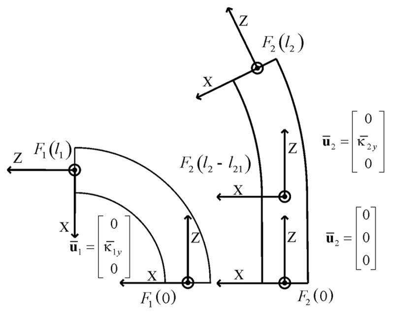
where ${\kappa }_f={\left[\begin{array}{cc}{\kappa }_{fx}& {\kappa }_{fy}\end{array}\right]}^T$ is the resultant curvature of the combined tubes, ${\overline{\kappa }}_i={\left[\begin{array}{cc}{\overline{\kappa }}_{xi}& {\overline{\kappa }}_{yi}\end{array}\right]}^T$ is the initial curvature of tube i prior to assembly, and $K_i=E_i{I}_i\left[\begin{array}{cc}1& 0\\ 0& 1\end{array}\right]$ is the stiffness matrix for tube i, with I_i being the tube cross section moment of inertia [10]. To apply (1), all of the κ̄_i must be expressed in the same coordinate frame. This is done, as shown in Fig. 1, by assigning a frame F_i(0) to the base of tube i, such that the z-axis of F_i(0) is tangent to the tube and the y-axis is aligned with the tube’s initial curvature vector. When the tubes are assembled, the frames F_i(0) are initially coincident with each other and with a stationary world frame W(0) (not shown). As each tube is rotated by an angle θ_i about the common z-axis, the frames F_i(0) are related to the world frame by F_i(0) = R(z, θ_i)W(0). Since the frames F_i(0) are chosen such that the initial curvature is entirely in the direction of the y-axis, the curvature of tube i in frame W(0) can be written as

$${\overline{\kappa }}_i^{W(0)}={\left[-\Vert {\overline{\kappa }}_i^{F_i(0)}\Vert sin\left({\theta }_i\right)\Vert {\overline{\kappa }}_i^{F_i(0)}\Vert cos\left({\theta }_i\right)\right]}^T$$ (2)

The application of mapping #1 for each type of fundamental element follows.

1. Individual Tubes: When a tube’s bending stiffness is greatly exceeded by that of its outer neighbor, it is treated individually and the curvature model (1) does not need to be applied. Its curvature is given by

   $${\widehat{\kappa }}_i^{W(0)}={\left[-\Vert {\overline{\kappa }}_i^{F_i(0)}\Vert sin\left({\theta }_i\right)\Vert {\overline{\kappa }}_i^{F_i(0)}\Vert cos\left({\theta }_i\right)\right]}^T.$$ (3)
2. Balanced Stiffness Tube Pair: The composite curvature for these tubes is computed using (1). The resulting map for this type of element is

   $${\left[\begin{array}{c}{\widehat{\kappa }}_{xi}\\ {\widehat{\kappa }}_{yi}\end{array}\right]}^{W(0)}=\frac{1}{K_{1i}+K_{2i}}\left[\begin{array}{c}-K_{1i}\Vert {\overline{\kappa }}_{1i}^{F_i}\Vert sin\left({\theta }_{1i}\right)-K_{2i}\Vert {\overline{\kappa }}_{2i}^{F_i}\Vert sin\left({\theta }_{2i}\right)\\ K_{1i}\Vert {\overline{\kappa }}_{1i}^{F_i}\Vert cos\left({\theta }_{1i}\right)+K_{2i}\Vert {\overline{\kappa }}_{2i}^{F_i}\Vert cos\left({\theta }_{2i}\right)\end{array}\right],$$ (4)

   and its composite stiffness is K̂_i = K_1i + K_2i.

B. Mapping Input Curves to Needle Arcs

The maximum number of needle arcs corresponds to the sum of piecewise constant curvature segments of all the tubes, n. As the extensions of the tubes vary, however, the actual number of arcs and the sequence of arcs from base to tip varies as well. This is treated here by assuming that there are always n arcs, but that some may be of zero arc length. For any given needle design, there will be a finite number of sequences of these n arcs. As will be demonstrated in the example section of the paper, this mapping must encode each extension-length dependent sequence of needle arcs. The curvature of each is computed using (1) applied to all input curves within the arc length.

C. Mapping Needle Arcs to Tip Frame

From [10], the transformation for a single arc is

$$T\left({\kappa }_x,{\kappa }_y,s\right)=\left[\begin{array}{cccc}\frac{{\kappa }_x^2+{\kappa }_y^{2}cos\left(s\Vert \kappa \Vert \right)}{{\Vert \kappa \Vert }^2}& \frac{{\kappa }_x{\kappa }_y\left(1-cos\left(s\Vert \kappa \Vert \right)\right)}{{\Vert \kappa \Vert }^2}& \frac{sin\left(s\Vert \kappa \Vert \right){\kappa }_y}{\Vert \kappa \Vert }& \frac{{\kappa }_y\left(1-cos\left(s\Vert \kappa \Vert \right)\right)}{{\Vert \kappa \Vert }^2}\\ \frac{{\kappa }_x{\kappa }_y\left(1-cos\left(s\Vert \kappa \Vert \right)\right)}{{\Vert \kappa \Vert }^2}& \frac{{\kappa }_y^2+{\kappa }_x^{2}cos\left(s\Vert \kappa \Vert \right)}{{\Vert \kappa \Vert }^2}& -\frac{sin\left(s\Vert \kappa \Vert \right){\kappa }_x}{\Vert \kappa \Vert }& -\frac{{\kappa }_x\left(1-cos\left(s\Vert \kappa \Vert \right)\right)}{{\Vert \kappa \Vert }^2}\\ -\frac{sin\left(s\Vert \kappa \Vert \right){\kappa }_y}{\Vert \kappa \Vert }& \frac{sin\left(s\Vert \kappa \Vert \right){\kappa }_x}{\Vert \kappa \Vert }& cos\left(s\Vert \kappa \Vert \right)& \frac{sin\left(s\Vert \kappa \Vert \right)}{\Vert \kappa \Vert }\\ 0& 0& 0& 1\end{array}\right]$$ (5)

The needle tip frame can then be written as a concatenation of all of the arc transformations,

$$W^{W(0)}(l_m)=T\left({\kappa }_{x1},{\kappa }_{y1},s_1\right)\cdots T\left({\kappa }_{xn},{\kappa }_{yn},s_n\right).$$ (6)

III. Inverse Kinematics

Solving the inverse kinematics relies on inverting the sequence of mappings described by Figure 2. While the first mapping between tube parameters and input curves is nonlinear, it can always be explicitly inverted. The second mapping from tube input curves to needle arcs is linear, but is not square since the number of needle arcs can exceed the number of input curves. Furthermore, the tube input curves are constrained by the curvatures and stiffnesses of the individual tubes. It is therefore advantageous to employ a generalized inverse Jacobian method to invert the second and third mappings since tube property constraints can be enforced via projection on the self motion manifold.

A. Inverting the Tube Parameters to Input Curves Map

The inverse can be performed explicitly for individual tubes and balanced stiffness pairs. Each is treated below.

1. Individual Tubes: The inverse is trivially obtained from (3) to be

   $${\theta }_i=\text{atan}2\left(-{\widehat{\kappa }}_{xi},{\widehat{\kappa }}_{yi}\right).$$ (7)

2. Balanced Stiffness Tube Pair: The resulting curvature of the tube pair is in a direction obtained by rotating the y-axis of W(0) by an angle α_i about the z-axis.

This angle is defined as

$${\alpha }_i=\text{atan}2\left(-{\widehat{\kappa }}_{xi},{\widehat{\kappa }}_{yi}\right).$$ (8)

Equation (4) can be inverted to yield two solutions since equal clockwise and counterclockwise relative rotations of the tube pair produce the same curvature,

$$\begin{array}{l}{\theta }_{2i}=\pm {cos}^{-1}\left(\frac{-{\left(K_{1i}\Vert {\overline{\kappa }}_{1i}\Vert \right)}^2+{\left(K_{2i}\Vert {\overline{\kappa }}_{2i}\Vert \right)}^2+{\Vert {\widehat{\kappa }}_i\Vert }^2{(K_{1i}+K_{2i})}^2}{2\Vert {\widehat{\kappa }}_i\Vert \Vert {\overline{\kappa }}_{2i}\Vert (K_{1i}+K_{2i})K_{2i}}\right)+{\alpha }_i,\\ {\theta }_{1i}={\theta }_{2i}-\text{atan}2\left(\pm \sqrt{1-c^2},c\right)\end{array}$$ (9)

where c = cos(θ_2i − θ_1i) and is given by

$$c=\frac{{\Vert {\widehat{\kappa }}_i\Vert }^2{\left(K_{1i}+K_{2i}\right)}^2-{\left(K_{1i}\Vert {\overline{\kappa }}_{1i}\Vert \right)}^2-{\left(K_{2i}\Vert {\overline{\kappa }}_{2i}\Vert \right)}^2}{2K_{1i}{K}_{2i}\Vert {\overline{\kappa }}_{1i}\Vert \Vert {\overline{\kappa }}_{2i}\Vert }.$$ (10)

B. Jacobian of Input Curve to Needle Arc Mapping

The m tube input curves (κ̂_x(s), κ̂_y (s), l)_i are mapped to the n≥m needle arcs (κ_x, κ_y, s)_j using the linear map of (1). Its derivative is denoted by J₂ which satisfies

$$\left[\begin{array}{c}{\left({\stackrel{.}{\kappa }}_x,{\stackrel{.}{\kappa }}_y,\stackrel{.}{s}\right)}_1^T\\ ⋮\\ {\left({\stackrel{.}{\kappa }}_x,{\stackrel{.}{\kappa }}_y,\stackrel{.}{s}\right)}_n^T\end{array}\right]=J_2\left[\begin{array}{c}{\left({\stackrel{.}{\widehat{\kappa }}}_x(s),{\stackrel{.}{\widehat{\kappa }}}_y(s),i\right)}_1^T\\ ⋮\\ {\left({\stackrel{.}{\widehat{\kappa }}}_x(s),{\stackrel{.}{\widehat{\kappa }}}_y(s),i\right)}_m^T\end{array}\right].$$ (11)

C. Jacobian of Needle Arc to Tip Frame Mapping

Given the transformation for a single arc in (5), the instantaneous spatial velocity at the arc tip is given by the twist, $V^s={\left[\begin{array}{cc}{v}^s& {\omega }^s\end{array}\right]}^T$ [8]. The matrix form V̂^s is given by

$${\widehat{V}}^s=\stackrel{.}{T}{T}^{-1}.$$ (12)

Expressing (12) in vector form defines the spatial Jacobian J_a for a single arc,

$$V^s=J_a{\left[{\stackrel{.}{\kappa }}_x,{\stackrel{.}{\kappa }}_y,\stackrel{.}{s}\right]}^T,$$ (13)

where the Jacobian is given by

$$\begin{array}{l}{J}_a=\left[{\left(\frac{\partial T}{\partial {\kappa }_x}{T}^{-1}\right)}^{\vee }{\left(\frac{\partial T}{\partial {\kappa }_y}{T}^{-1}\right)}^{\vee }{\left(\frac{\partial T}{\partial s}{T}^{-1}\right)}^{\vee }\right]\\ =\left[\begin{array}{ccc}0& -\Vert \kappa \Vert \left(1-cos\left(s\Vert \kappa \Vert \right)\right)& 0\\ \Vert \kappa \Vert \left(1-cos\left(s\Vert \kappa \Vert \right)\right)& 0& 0\\ {\kappa }_x\left(s\Vert \kappa \Vert -sin\left(s\Vert \kappa \Vert \right)\right)& {\kappa }_y\left(s\Vert \kappa \Vert -sin\left(s\Vert \kappa \Vert \right)\right)& {\Vert \kappa \Vert }^3\\ s{\kappa }_x^2\Vert \kappa \Vert +{\kappa }_y^{2}sin\left(s\Vert \kappa \Vert \right)& {\kappa }_x{\kappa }_y\left(s\Vert \kappa \Vert -sin\left(s\Vert \kappa \Vert \right)\right)& {\kappa }_x{\Vert \kappa \Vert }^3\\ {\kappa }_x{\kappa }_y\left(s\Vert \kappa \Vert -sin\left(s\Vert \kappa \Vert \right)\right)& s{\kappa }_y^2\Vert \kappa \Vert +{\kappa }_x^{2}sin\left(s\Vert \kappa \Vert \right)& {\kappa }_y{\Vert \kappa \Vert }^3\\ -{\kappa }_y\Vert \kappa \Vert \left(1-cos\left(s\Vert \kappa \Vert \right)\right)& {\kappa }_x\Vert \kappa \Vert \left(1-cos\left(s\Vert \kappa \Vert \right)\right)& 0\end{array}\right]\frac{1}{{\Vert \kappa \Vert }^3}.\end{array}$$ (14)

For a needle consisting of n arcs, the Jacobian of the mapping is

$$J_3=\left[J_{a1},{\text{Ad}}_1{J}_{a2},\cdots ,{\text{Ad}}_{n-1}{J}_{an}\right],$$ (15)

in which Ad_j is the adjoint transformation for arcs 1…j,

$${Ad}_j={\left[\begin{array}{cc}{R}_{1j}& {p_{1j}}^{\wedge }{R}_{1j}\\ 0& R_{1j}\end{array}\right]}_{1,\dots j}.$$ (16)

D. Pseudo Inverse Solution

The Jacobians of mappings #2 and #3 are combined to yield the following

$$V^s=J_{32}\left[\begin{array}{c}{\left({\stackrel{.}{\widehat{\kappa }}}_x(s),{\stackrel{.}{\widehat{\kappa }}}_y(s),i\right)}_1^T\\ ⋮\\ {\left({\stackrel{.}{\widehat{\kappa }}}_x(s),{\stackrel{.}{\widehat{\kappa }}}_y(s),i\right)}_m^T\end{array}\right],$$ (17)

in which J₃₂ = J₃J₂. This relation is inverted using the generalized inverse,

$$\left[\begin{array}{c}{\left({\stackrel{.}{\widehat{\kappa }}}_x(s),{\stackrel{.}{\widehat{\kappa }}}_y(s),i\right)}_1^T\\ ⋮\\ {\left({\stackrel{.}{\widehat{\kappa }}}_x(s),{\stackrel{.}{\widehat{\kappa }}}_y(s),i\right)}_m^T\end{array}\right]=J_{32}^{+}{V}^s+\left(J_{32}^{+}{J}_{32}-I\right)\nabla h,$$ (18)

where $J_{32}^{+}=J_{32}^T{\left(J_{32}{J}_{32}^T\right)}^{-1}$ and ∇h is the gradient of a smooth positive definite function encoding constraints on tube input curve curvatures and extension lengths,

$$h=h\left({\left({\widehat{\kappa }}_x(s),{\widehat{\kappa }}_y(s),l\right)}_1,\dots ,{\left({\widehat{\kappa }}_x(s),{\widehat{\kappa }}_y(s),l\right)}_m\right).$$ (19)

This is illustrated in the example section.

E. Specifying Spatial Tip Velocity

To use (18) to compute the tube input curves, and subsequently the tube parameters, associated with a desired tip coordinate frame as given by (6), an expression for spatial velocity, V^s, is needed which relates the current and desired coordinate frames. For simplicity, the velocity profile is taken to be a constant velocity twist corresponding to the screw motion between the two frames T_a and T_b.

From [7], the direction of the screw axis, b, is given in matrix form by

$${[b]}^{\wedge }=\left(R_{ab}-I\right){\left(R_{ab}+I\right)}^{-1},$$ (20)

where R_ab is the rotation from the initial frame, R_a, to the final frame, R_b, given by

$$R_{ab}=R_b{R}_a^T.$$ (21)

The unit magnitude angular velocity from T_a to T_b is then

$${\omega }^s=b/\left|\right|b\left|\right|,$$ (22)

and the rotation angle between the frames about ω^s is

$${\theta }_{ab}=2{tan}^{-1}\left(\left|\right|b\left|\right|\right).$$ (23)

The translation between the two frames, d, is given by

$$d=p_b-p_a.$$ (24)

The vector, d^*, the projection of d onto a plane perpendicular to ω^s, is

$$d^{\ast }={\omega }^s\times \left(d\times {\omega }^s\right).$$ (25)

Also from [7], a point on the screw axis is given by

$$q^{\ast }=\frac{b\times d^{\ast }}{{\left|\right|b\left|\right|}^2}+d^{\ast }.$$ (26)

and the screw pitch is given by

$$h=sgn\left(\left(d-d^{\ast }\right)·{\omega }^s\right)\frac{\left|\right|d-d^{\ast }\left|\right|}{{\theta }_{ab}}.$$ (27)

This corresponds to a twist for use in (18) given by

$$\left[\begin{array}{c}{v}^s\\ {\omega }^s\end{array}\right]=\left[\begin{array}{c}-\left(b/\left|\right|b\left|\right|\right)\times q^{\ast }+h\left(b/\left|\right|b\left|\right|\right)\\ b/\left|\right|b\left|\right|\end{array}\right]$$ (28)

which can be numerically integrated from t = 0 to t = θ_ab. When the initial and desired tip frames are related by a pure translation, the spatial velocity is given by

$$\left[\begin{array}{c}{v}^s\\ {\omega }^s\end{array}\right]=\left[\begin{array}{c}d\\ 0\end{array}\right]$$ (29)

and integration in this case is from t = 0 to t = 1.

IV. Examples

Two examples are presented in this section. The first example is of a needle comprised of three tubes arranged as a balanced stiffness, dominating stiffness design similar to the design of Figure 1. The second example is comprised of six tubes arranged as a sequence of three balanced stiffness tube pairs.

A. Example #1

The balanced stiffness, dominating stiffness design indicates that m = 2. The innermost tube has two sections of constant curvature – zero curvature over the proximal portion and a finite nonzero curvature, ||κ̂|| = κ̂₀, over the distal portion of length l₂₁. As a result, the needle will consist of n = 3 arcs. The mapping between tube input curves and needle arcs is given by

$$\begin{array}{l}{s}_1=max\left(0,l_2-l_{21}\right)\\ s_2=l_1-max\left(0,l_2-l_{21}\right)\\ s_3=l_2-l_1\end{array}$$ (30)

$$\left[\begin{array}{c}{\kappa }_1\\ {\kappa }_2\\ {\kappa }_3\end{array}\right]=\left[\begin{array}{cc}{c}_1& 0\\ c_1& c_2\\ 0& 1\end{array}\right]\left[\begin{array}{c}{\widehat{\kappa }}_1\\ {\widehat{\kappa }}_2\end{array}\right],$$ (31)

where c_i = K̂_i/(K̂₁ + K̂₂). The Jacobian J₂ is obtained by differentiating these expressions resulting in

$$J_2=\left[\begin{array}{cccccc}{c}_1& 0& 0& 0& 0& 0\\ 0& c_1& 0& 0& 0& 0\\ 0& 0& 0& 0& 0& U(l_2-l_{21})\\ c_1& 0& 0& c_2& 0& 0\\ 0& c_1& 0& 0& c_2& 0\\ 0& 0& 1& 0& 0& -U(l_2-l_{21})\\ 0& 0& 0& 1& 0& 0\\ 0& 0& 0& 0& 1& 0\\ 0& 0& -1& 0& 0& 1\end{array}\right],$$ (32)

where U is the unit step function. The Jacobian J₃ is computed using (14) and (15).

To enforce the tube constraints on curvature, the following positive definite function is used for (19).

$$h={\left({\widehat{\kappa }}_{x1}^2+{\widehat{\kappa }}_{y1}^2-{{\widehat{\kappa }}_{1,\text{des}}}^2\right)}^2+{\left({\widehat{\kappa }}_{x2}^2+{\widehat{\kappa }}_{y2}^2-{{\widehat{\kappa }}_{2,\text{act}}}^2\right)}^2,$$ (33)

In the first term, κ̂_1,des is selected as a value of curvature that the balanced stiffness pair can achieve for some relative rotation angle. In the second term, κ̂_2,act is the actual value of curvature of the distal portion of the inner tube. After integrating (18) to the goal configuration, if the curvatures have not converged sufficiently to the desired values, V^s is set to zero and integration continues until the convergence criteria is satisfied.

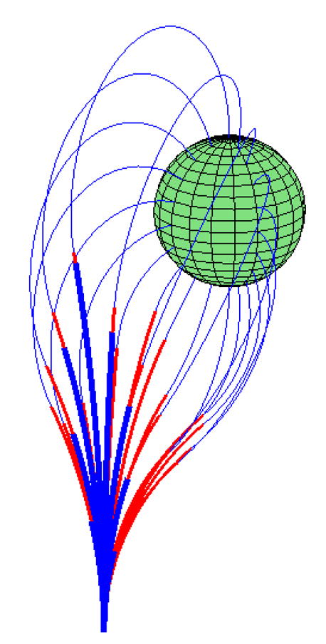
Figure 3 depicts the inverse kinematic solutions for the example needle tracing a portion of a sphere’s surface. The convergence criteria for κ̂_2,act was ±.005cm⁻¹. The colors indicate the three arcs of the needle. The red section corresponds to the overlap between the balanced stiffness pair and the nonzero curvature portion of the inner tube.

Figure 3.

Needle of example 1 tracing the surface of a sphere.

B. Example #2

This design is comprised of three balanced stiffness tube pairs. The two inner balanced stiffness pairs are constructed similarly to the dominating stiffness element in the previous example with sections of zero curvature at their proximal ends and variable curvature at their distal ends. As a result, the needle consists of n = 5 arcs. These arcs can be arranged in three different overlap configurations as shown in Figure 4 where changes in curvature along a tube are indicated by changes in shading.

Figure 4.

Three possible arrangements of needle arcs for example 2.

The needle is in configuration (a) when l₃ − l₃₁ > l₁, in configuration (b) when l₁ > l₃ − l₃₁ > l₂ − l₂₁, and in configuration (c) when l₂ − l₂₁ > l₃ − l₃₁. It should be noted that configuration (c) is only possible if l₃₁ > l₂₁.

The second mapping for each configuration is as follows:

$$(a)\left[\begin{array}{c}{\kappa }_1\\ {\kappa }_2\\ {\kappa }_3\\ {\kappa }_4\\ {\kappa }_5\end{array}\right]=\left[\begin{array}{ccc}{a}_1& 0& 0\\ a_1& a_2& 0\\ 0& b_2& 0\\ 0& b_2& b_3\\ 0& 0& 1\end{array}\right]\left[\begin{array}{c}{\widehat{\kappa }}_1\\ {\widehat{\kappa }}_2\\ {\widehat{\kappa }}_3\end{array}\right]$$ (34)

$$\begin{array}{ll}{s}_1=max\left(0,l_2-l_{21}\right)\hfill & s_4=l_2-l_1-max\left(0,l_3-l_{31}-l_1\right)\hfill \\ s_2=l_1-max\left(0,l_2-l_{21}\right)\hfill & s_5=l_3-l_2\hfill \\ s_3=max\left(0,l_3-l_{31}-l_1\right)\hfill & \hfill \end{array}$$ (35)

$$(b)\left[\begin{array}{c}{\kappa }_1\\ {\kappa }_2\\ {\kappa }_3\\ {\kappa }_4\\ {\kappa }_5\end{array}\right]=\left[\begin{array}{ccc}{a}_1& 0& 0\\ a_1& a_2& 0\\ a_1& a_3& a_3\\ 0& b_2& b_3\\ 0& 0& 1\end{array}\right]\left[\begin{array}{c}{\widehat{\kappa }}_1\\ {\widehat{\kappa }}_2\\ {\widehat{\kappa }}_3\end{array}\right]$$ (36)

$$\begin{array}{l}\begin{array}{l}{s}_1=max\left(0,l_2-l_{21}\right)\hfill \\ s_2=max\left(0,l_3-l_{31}-max\left(0,l_2-l_{21}\right)\right)\hfill \\ s_3=l_1-max\left(0,l_3-l_{31}-max\left(0,l_2-l_{21}\right)\right)-max\left(0,l_2-l_{21}\right)\hfill \\ s_4=l_2-l_1\hfill \\ s_5=l_3-l_2\hfill \end{array}\hfill \end{array},$$ (37)

$$(c)\left[\begin{array}{c}{\kappa }_1\\ {\kappa }_2\\ {\kappa }_3\\ {\kappa }_4\\ {\kappa }_5\end{array}\right]=\left[\begin{array}{ccc}{a}_1& 0& 0\\ a_1& 0& a_3\\ a_1& a_3& a_3\\ 0& b_2& b_3\\ 0& 0& 1\end{array}\right]\left[\begin{array}{c}{\widehat{\kappa }}_1\\ {\widehat{\kappa }}_2\\ {\widehat{\kappa }}_3\end{array}\right]$$ (38)

$$\begin{array}{ll}{s}_1=max\left(0,l_3-l_{31}\right)\hfill & s_4=l_2-l_1\hfill \\ s_2=max\left(0,l_2-l_{21}\right)-max\left(0,l_3-l_{31}\right)\hfill & s_5=l_3-l_2\hfill \\ s_3=l_1-max\left(0,l_2-l_{21}\right)\hfill & \hfill \end{array},$$ (39)

where a_i = K̂_i/(K̂₁ + K̂₂ + K̂₃) and b_i = K̂_i/(K̂₂ + K̂₃).

The Jacobian J₂ is straightforward to compute, but is not given here due to space limitations.

The positive definite function used in integrating (18) is given by

$$h=\sum _{i=1}^3{\left({\widehat{\kappa }}_{xi}^2+{\widehat{\kappa }}_{yi}^2-{{\widehat{\kappa }}_{i,\text{des}}}^2\right)}^2+{\left(l_2-l_1-{\lambda }_1\right)}^2+{\left(l_3-l_2-{\lambda }_2\right)}^2,$$ (40)

where λ₁ and λ₂ are positive constants. The latter terms enforce the assumption of telescoping extension, l₁ ≤ l₂ ≤ l₃.

The figure below shows the results for this needle design tracing the same path on the surface of a sphere as in the first example. As before, sections of overlapping curvature between balanced pairs are shown in red.

V. Conclusion

Concentric tube needles represent a novel and exciting approach to enhancing the steerability of needles for percutaneous procedures. This paper presents a methodology for efficient computation of the individual tube rotations and extensions needed to advance a concentric tube needle along a desired insertion path. These techniques can be adapted for intervention planning and for closed-loop control.

Figure 5.

Needle of example 2 tracing the surface of a sphere.

Figure 6.

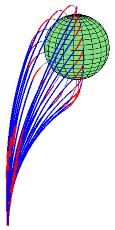
Fig. 1. Tube coordinate frames and initial curvatures.

References

- 1.Antman SS. Nonlinear problems of elasticity. Springer Verlag; New York: 1995. [Google Scholar]
- 2.Chirikjian GS. A Modal Approach to Hyper-redundant Manipulator Kinematics. IEEE Trans On Robotics and Automation. 1994;10(3):343–354. [Google Scholar]
- 3.Huang MZ, Varma H. Optimal Rate Allocation in Kinematically Redundant Manipulators – The Dual Projection Method. Proc. IEEE Intl. Conf. on Robotics and Automation; 1993. [Google Scholar]
- 4.Jones B, Walker ID. Kinematics for Multi-Section Continuum Robots. IEEE Transactions on Robotics. 2006;22(1):45–53. [Google Scholar]
- 5.Klein CA, Huang CH. Review of Pseudoinverse Control for Use with Kinematically Redundant Manipulators. IEEE Transactions of Systems, Man, and Cybernetics. 1983;13(3):245–250. [Google Scholar]
- 6.Liégeois A. Automatic Supervisory Control of the Configuration and Behavior of Multibody Mechanisms. IEEE Transactions on Systems, Man, and Cybernetics. 1977;7(12):868–871. [Google Scholar]
- 7.McCarthy JM. An Introduction to Theoretical Kinematics. The MIT Press; Cambridge, Massachusetts: 1990. [Google Scholar]
- 8.Murray R, Li Z, Sastry S. A Mathematical Introduction to Robotic Manipulation. CRC Press; Boca Raton, Florida: 1994. [Google Scholar]
- 9.Robinson G, Davies JBC. Continuum Robots – A State of the Art. Proc. IEEE Intl. Conf. on Robotics and Automation; Detroit. May 1999; pp. 2849–2854. [Google Scholar]
- 10.Sears P, Dupont P. A Steerable Needle Technology Using Curved Concentric Tubes. IEEE/RSJ Int. Conference on Intelligent Robots and Systems; Beijing. 2006. pp. 2850–2856. [Google Scholar]
- 11.Simaan N, Taylor R, Flint P. A dexterous system for laryngeal surgery. Proc. IEEE Intl. Conf. on Robotics and Automation; New Orleans. April 2004; pp. 351–357. [Google Scholar]
- 12.Webster RJ, Okamura AM, Cowan NJ. Toward Active Cannulas: Miniature Snake-Like Surgical Robots. IEEE/RSJ Int. Conference on Intelligent Robots and Systems; Beijing. 2006. pp. 2857–2863. [Google Scholar]
- 13.Loser M. Dr Ing Dissertation. Microsystems Technology, Univ. of Freiburg; Germany: 2005. A New Robotic System for Visually Controlled Percutaneous Interventions under X-ray Fluoroscopy or CT-imaging. [Google Scholar]