Mapping shape quantitative trait loci using a radius-centroid-contour model

Abstract

As the consequence of complex interactions between different parts of an organ, shape can be used as a predictor of structural–functional relationships implicated in changing environments. Despite such importance, however, it is no surprise that little is known about the genetic detail involved in shape variation, because no approach is currently available for mapping quantitative trait loci (QTLs) that control shape. Here, we address this problem by developing a statistical model that integrates the principle of shape analysis into a mixture-model-based likelihood formulated for QTL mapping. One state-of-the-art approach for shape analysis is to identify and analyze the polar coordinates of anatomical landmarks on a shape measured in terms of radii from the centroid to the contour at regular intervals. A procrustes analysis is used to align shapes to filter out position, scale and rotation effects on shape variation. To the end, the accurate and quantitative representation of a shape is produced with aligned radius-centroid-contour (RCC) curves, that is, a function of radial angle at the centroid. The high dimensionality of the RCC data, crucial for a comprehensive description of the geometric feature of a shape, is reduced by principal component (PC) analysis, and the resulting PC axes are treated as phenotypic traits, allowing specific QTLs for global and local shape variability to be mapped, respectively. The usefulness and utilization of the new model for shape mapping in practice are validated by analyzing a mapping data collected from a natural population of poplar, Populus szechuanica var tibetica, and identifying several QTLs for leaf shape in this species. The model provides a powerful tool to compute which genes determine biological shape in plants, animals and humans.

Introduction

Tremendous variation in morphological shape provides a fuel for the evolution of biological function and the formation of new species that best adapt to a specific environment (Albertson et al., 2005; Klingenberg, 2010; Koenig and Sinha, 2010). Genes are thought to have an important role in controlling phenotypic variation in shape (van der Knapp et al., 2002; Tanksley, 2004; Scarpella et al., 2010); according to quantitative genetic analyses in animals, shape may have a heritability of 0.60–0.70 (Klingenberg and Leamy, 2001; Monteiro et al., 2002; Klingenberg, 2003; Mezey and Houle, 2005; Gilchrist and Crisafulli, 2006). With the development of genotyping techniques, genetic mapping that dissects phenotypic variation into individual quantitative trait loci (QTLs) (Lander and Botstein, 1989) has been used to detect specific QTLs for morphological shape in the mouse, Drosophila and tomato, providing many promising results (Weber et al., 1999; Klingenberg et al., 2001, 2004, 2012; van der Knapp et al., 2002; Mezey et al., 2005; Leamy et al., 2008). More recently, (Fu et al., 2010) developed a binary model for shape mapping based on computer-simulated black and white shape data. (Langlade et al., 2005) used 19 representative points for a leaf to map the QTLs that control the allometry of leaf shape and pioneered the integration of shape QTLs with interspecific divergence and evolution.

Many of these shape genetic studies are based on a simple geometric analysis and, thus, do not intend to resolve the inherently complicated structure of a biological shape. For example, simple morphological measures for length, width, height, ratio and angle do not separate size and shape clearly (Rohlf and Marcus, 1993; van der Knapp et al., 2002), although these two aspects perform different biological functions (Tanksley, 2004). In addition, some more advanced genetic analyses of shape mostly focus on drastic morphological changes, but do not allow a quantitative description of detailed structures of organ morphology, such as leaf margins that can be entire, serrated or lobed (reviewed in Klingenberg, 2010).

As an important approach for shape analysis, geometric morphometrics has a capacity to quantify each piece of subtle variation that accumulatively contributes to shape (Klingenberg, 2010). By analyzing the polar coordinates of anatomical landmarks, shape analysis based on the geometric morphometrics model retains geometric information from digitized data and relates abstract, multivariate results to the physical structure of the original specimens (Adams et al., 2004; Slice, 2007). The development of image and digital technologies has greatly facilitated shape recognition and shape registration based on the theory that a shape can be represented by a number of carefully selected and coded image patches extracted from images taken from different viewpoints (Belongie et al., 2002). The recent years have seen the development of new technologies used to analyze and interpret the molecular, mechanical and dynamic mechanisms that form shape (Nath et al., 2003; Rolland-Lagan et al., 2003; Coen et al., 2004). Coen et al. (2004) used clonal analysis techniques to study the dynamic relationship between gene expression pattern and leaf shape (Rolland-Lagan et al., 2005). Liang and Mahadevan (2009) capitalized on a combination of scaling, stability and asymptotic analysis to quantify leaf shape and the conditions that cause different morphologies of leaves.

As a first step of our shape gene identification project, here, we developed a model for studying the genetic mechanisms of morphological shape by mapping specific QTLs involved in shape variation. This model integrates existing geometric morphometrics analysis into a framework for QTL mapping through a series of statistical bridges. By measuring radii from the centroid to the contour at regular intervals, we quantify the geometric features of a shape and further use a procrustes analysis to align shapes with different poses, scales and rotations. The high dimension of shape data measured by a radius-centroid-contour (RCC) analysis is reduced by principal component (PC) analysis producing orthogonal PC axes that capture global and local variability, respectively. Based on the PC axes of RCC values, a QTL-mapping model is derived and then the QTL effects detected on shape structure are transformed back to image domains in order to intuitively visualize how QTLs affect shape variation. To demonstrate the utility and usefulness of the new model, we used it to analyze a mapping population of a poplar species, leading to the detection of several significant QTLs that govern leaf shape. The new model combines the strengths from genetic mapping and shape analysis, providing a powerful tool for the genome-wide identification of QTLs with varying sizes of genetic effects on shape diversity.

Materials and methods

The theory of shape analysis has well been established by (Kendall, 1984), in which a finite number of landmarks are used to represent a shape of an object. According to Kendall's definition, ‘shape is all the geometrical information that remains when location, scale and rotational effects are filtered out from an object.' Here, we integrate this theory into the genetic mapping framework that is used to characterize the structural, functional, and developmental features of shape.

Statistical design

A segregating population is a prerequisite for mapping trait QTLs. Consider a natural population from which a sample of n individuals is drawn randomly. All these individuals are genotyped for a panel of molecular markers. Meanwhile, the shape of an organ, such as leaf, is measured for each individual by taking a photograph of representative leaves. It is likely that a set of QTLs controls shape, forming a total of J genotypes. Although we cannot observe these QTL genotypes directly, they can be inferred from the markers (M) that are linked to the QTLs. For this reason, a basic statistical model for QTL mapping is a mixture model, in which each observation Y is assumed to have arisen from one of the J QTL genotypes, each genotype (j) being modeled from a density function (frequently a normal distribution is assumed). Thus, the likelihood of Y is expressed as

where ω is composed of mixture proportions ω_j|i of individual i carrying a QTL genotype j, φ_j is the expectation parameter vector specific to a QTL genotype j, and η_i is the variance–covariance parameter common to all genotype groups, and f_j(Y_i|φ_j,η_i) is the probability density function of observations for individual i at QTL genotype j. For a natural population, the mixture proportions (ω_j|i) of each QTL genotype j in likelihood (1) are described in terms of allele frequencies at the markers and QTLs and their linkage disequilibria (LD) (Wang and Wu, 2004). The size of LD reflects the degree to which the markers and QTLs are associated.

To capture the complicated structure of a shape, we used a high dimension of pixels to describe its boundary and detailed inner feature. A vector of representation for the shape can be denoted as coordinates (x(s), y(s)) (s=0, 1,…, m—1) extracted from a digital image, where m is the number of coordinates, determining the accuracy of shape representation. The steps for shape analysis with digital images are described below.

Shape alignment

All shapes need to be aligned, in order to minimize variation caused by pose. Shape alignment is a process that is used to establish a coordinate reference for all shapes with respect to position, scale and rotation, commonly known as pose. An orthogonal procrustes analysis is used to undertake this alignment (Gower and Dijksterhuis, 2004).

To make shape representation invariant to translation, we shift all shapes to their centroids by

where (x_c, y_c) is the centroid of a shape, which is defined as

By using the new coordinate system (x₁(s), y₁(s)), all shapes have the origin at the centroid and thus eliminate any influence caused by position.

To filter a scale effect, we normalized all shapes by dividing each shape by its Euclidean or Frobenius norm, which produces the normalized shape:

The last and most complicated step for shape alignment is to remove the rotation effect. The idea behind is to rotate each shape one by one so that they can be close to a reference shape as much as possible. We use the Euclidean or Frobenius norm to measure the distance between two shapes. The smaller the Euclidean norm, the closer they are. In addition, the average of all shapes is used as the reference shape (denoted as ). Now, we assume

is the rotation matrix; after multiplying it on the right-hand side of (4), the shape gets rotated θ angles clockwise. Denote Z as (x₂(s), y₂(s)). By definition, we hope to solve Q by minimizing

where the first part does not contain Q, so that we only need to maximize trace(). By singular value decomposition, there exist orthogonal matrices U and V and diagonal matrix D such that . Hence,

where H=V^TQU is an orthogonal matrix, d_l is the lth diagonal element of diagonal matrix D, and h_ll is the lth diagonal element of H. Therefore, is maximized when H=I. This is equivalent to Q=VU^T.

It can be seen from the above derivation that we should multiply the right-hand side of (x₂(S),y₂(S)) by VU^T to rotate a shape to be close to the average of all shapes. The three steps described above are repeated and iterated until the rotated shapes provide the best fit of differences among all shapes caused by pose. We use () (s=0, 1, …, m−1) to denote final coordinates of each shape after alignment.

Shape representation

As a popular contour-based method, we use landmarks for shape representation. Landmarks are a set of points on the boundary assigned by either geometrical property (such as high curvature), or an extremum point, or specific biological meaning (Cootes et al., 1995; Belongie et al., 2002). To make a one-to-one correspondence between landmarks of one shape and all other shapes, we choose the same angle or the same arc length. We select points on the boundary spaced at equal radial angle θ=2π/m, where m is the number of points. This gives an accurate and robust description of shape. A shape can be described by RCC values (Belongie et al., 2002), that is,

which are used for QTL mapping.

Dimension reduction

Many approaches can be used to decompose the original m-dimensional space to a space of reduced dimension. Principal component analysis (PCA) is one of such powerful approaches by removing redundant information through mapping the high dimensional data to the subspace that best accounts for the distribution of the original pattern. Denote n shape data by R={r₁, r₂, …, r_n} in the R^m space, where r_i is the RCC curve of the ith leaf shape with length m. The average of these data is defined by

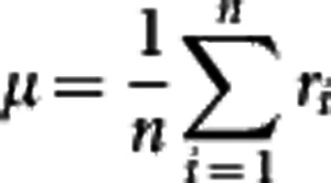and the maximum-likelihood estimation (MLE) of variance can be given by . Let X={r₁−μ, r₂−μ, …, r_n−μ }, then we have Σ_R=XX^T, a m × m matrix, which is too big to be manipulated practically. The main idea behind PCA is to maximize the variance by finding a certain number of orthogonal axes, called PCs, that is much fewer than m. Therefore, through PCA, we can use , where v_k (k=1, …, K) is the eigenvector of X^TX in terms of the kth PC, to model the likelihood (1). The first K of the largest PCs are chosen. Next, we will describe a procedure for LD mapping of QTLs using these PC values (Wang and Wu, 2004).

Linkage disequilibrium mapping

To map QTLs in a natural population, we need to implement LD as a parameter that links markers with QTLs. For clarity of model description, we assume one QTL controlling a shape that is associated with a marker, with two alleles M (with a probability p) and m (with a probability 1−p), through a LD, D. At the shape QTL, there are two alleles A (with a probability q) and a (with a probability 1−q) that form three genotypes, expressed as AA (denoted as 1), Aa (denoted as 2), and aa (denoted as 3). The marker and QTL form four haplotypes MA, Ma, mA and ma, with the frequencies denoted as p₁₁=pq+D, p₁₀=p(1−q)−D, p₀₁=(1−p)q−D, and p₀₀=(1−p)(1−q)+D, respectively, where max(−pq,−(1−p)(1−q))⩽D⩽min(p(1−q), (1−p)q). The haplotypes from maternal and paternal parents unite randomly to generate nine marker-QTL genotypes. The conditional probabilities of a given QTL genotype, conditional upon a marker genotype for individual j, expressed as ω_j|i in the likelihood (1), can be calculated (see Wang and Wu, 2004). The observations of three genotypes at the marker are denoted as n₁ for MM, n₂ for Mm and n₃ for mm.

The parameters that define the likelihood (1) are obtained by differentiating the likelihood with respect to each parameter, letting the derivative equal to zero, and then solving the log-likelihood equations. We implemented the EM algorithm to estimate the parameters. The E step is designed to calculate the posterior probability with which individual i carries QTL genotype j given its marker and phenotypic information, expressed as

Using the calculated posterior probabilities, the M step is derived to solve the haplotype frequencies expressed as

where θ=p₁₁p₀₀/(p₁₁p₀₀+p₁₀p₀₁). The iteration are repeated between including equation (6) and equations (7−12) until the estimates converge to stable values. These stables values are the maximum likelihood estimates (MLEs) of parameters.

Hypothesis tests

Based on likelihood (1), the significance of a shape QTL can be tested by using the following hypotheses:

H₀: μ_j≡μ ∀j=1, 2, 3

H₁: At least one of the equalities above does not hold; (13)

where the H₀ corresponds to the reduced model, in which the data can be fit by a single shape, and the H₁ corresponds to the full model, in which three QTL genotype-specific shapes exist to fit these data. The log-likelihood ratio (LR) of the full to reduced model is calculated as the test statistics for the above hypotheses. An empirical approach based on permutation tests is used to determine the critical threshold (Churchill and Doerge, 1994). The significance level was further corrected for multiple comparisons using Bonferroni's criterion.

After a significant QTL is found to exist, we need to test whether this QTL can be detected by a given marker using the hypotheses:

H₀: D=0 vs H₁: D≠0; (14)

where the H₀ corresponds to the reduced model, in which the marker and QTL are at the linkage equilibrium, and the H₁ corresponds to the full model, in which there is a LD between the marker and QTL. The test statistics for this hypothesis is calculated as χ²=2nD²/[p(1–p)q(1–q)], which is χ²-distributed with one degree of freedom. The significance level was corrected for multiple comparisons using Bonferroni's criterion.

Results

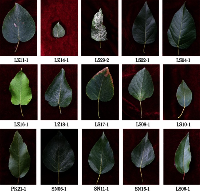
The new model was used to analyze leaf shape data for a mapping population of poplar, Populus szechuanica var. tibetica. Belonging to the Tacamahaca section, P. szechuanica is naturally distributed throughout the Tibet Plateau, growing in mountains at an altitude of 1100−4600 m, over a wide range of regions in Gansu, Shaanxi, Sichuan, Xizang and Yunnan Provinces of China (Hamzeh and Dayanandan, 2004). The wide ecological adaptation of this species, along with its pronounced variation in leaf size and shape (Figure 1), makes this species ideal to study the genetic variation of leaf morphology using molecular markers. The overall shape of leaf blade in P. szechuanica var. tibetica varies markedly from broadly ovate to ovate-orbicular to ovate-lanceolate. The bases of leaf blades are rounded, cuneate or shallowly cordate with glandular dentate margins at the first ciliate. Leaves grow from short branchlets with petioles 2.5−8 cm. A precise shape analysis approach is needed to identify and quantify such a diversity of leaf shape.

Figure 1.

A set of original leaf images (with IDs given at the bottoms) chosen from the mapping population for P. szechuanica var. tibetica, showing pronounced variation in leaf shape.

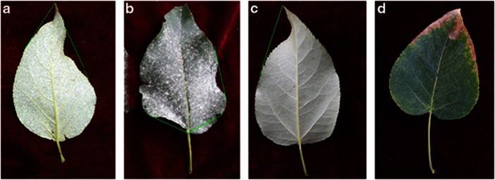
Langlade et al., 2005 pioneered a numerical analysis for shape variation in leaves by placing 19 key landmarks on the leaf margin and leaf mid-vein from digital images. However, joining these 19 points with straight lines can only capture the global feature of a leaf outline. The choice of sparse anatomical landmarks by this approach is extremely difficult when some leaves (see examples in Figures 2a–c) are abruptly curved. This part of leaf shape variation may be linked with some particular ecological function (Kessler and Sinha, 2004) and, therefore, should be taken into account. Furthermore, in (Langlade et al., 2005), a straight mid-vein was used to align leaf shapes (see their Figure 2). In our example, however, many leaves display a curved mid-vein (Figure 2d), making it difficult to align shapes using the mid-vein as a reference.

Figure 2.

Four typical leaf shapes detected from the mapping population. In (a–c), leaf margins are not always smoothly curved, as shown by green lines, which makes it difficult to determine anatomical landmarks on the leaf outlines using traditional approaches. In (d), the mid-vein is crooked, which cannot be used as a reference to align leaf shapes.

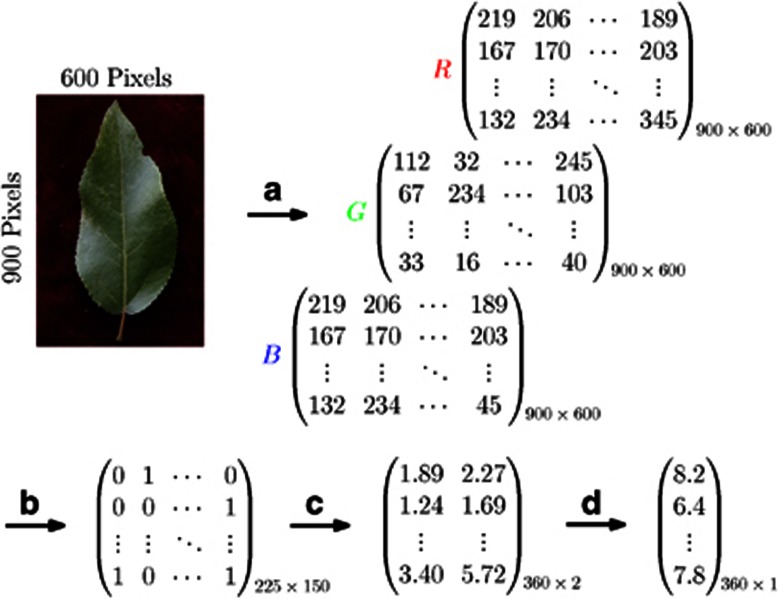
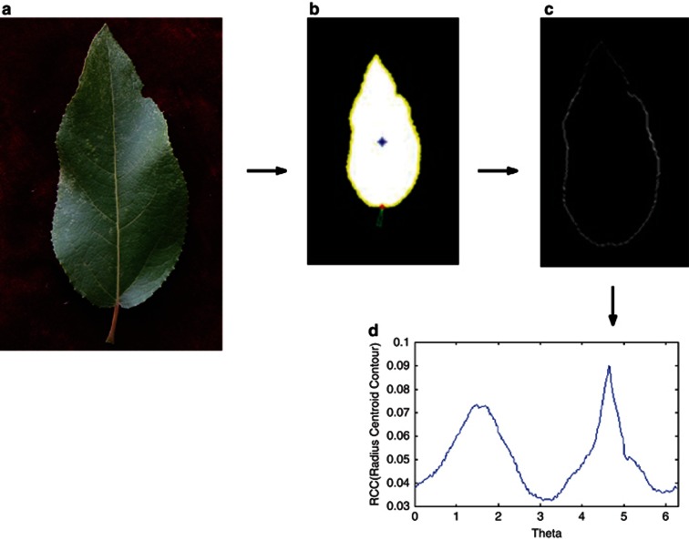
As a pilot study of shape mapping, we selected 107 trees randomly from a natural population of P. szechuanica var. tibetica, and from each tree, three representative leaves were sampled to take photos. The sampled trees were genotyped for 29 microsatellite markers to be used to detect leaf shape QTLs. By reading 600 × 900 pixels from a leaf digital image, we obtained three matrices for red, green and black colors that discern the object and background (Figure 3a), from which binary smaller matrix was generated to capture the leaf shape by recording its contour (Figure 3b). Using the procedure for shape alignment described in Materials and methods, we obtained a vector of 360 coordinates (s=0, 1, …, 359) to represent leaf shape. It turns out that 360 points can well describe the leaf boundary (Figures 3c and D). Figure 4 is the diagrammatic representation of several key steps (A, B, C and D) described in Figure 3. The 360 representative points shown in a vector (Figure 3d) can be actually expressed as a RCC curve (Figure 4d).

Figure 3.

The procedure of extracting leaf-shape information from a leaf image. In (a), the leaf is read by 900 × 600 pixels based on different colors, red (R), green (G) and black (B) for the object and background. In (b), the leaf outline is read as a 1/0 binary variable with a dimension-reduced matrix. In (c), the Cartesian coordinates of points on the leaf outline are calculated. In (d), all coordinates in (c) are expressed as single RCC values.

Figure 4.

Diagrammatic representation of the extracting procedure described in Figure 3. a–d in this figure correspond to those in Figure 3, respectively. The vector of RCC values in Figure 3d is expressed as a curve, which is a function of radial angle (θ) (see the text).

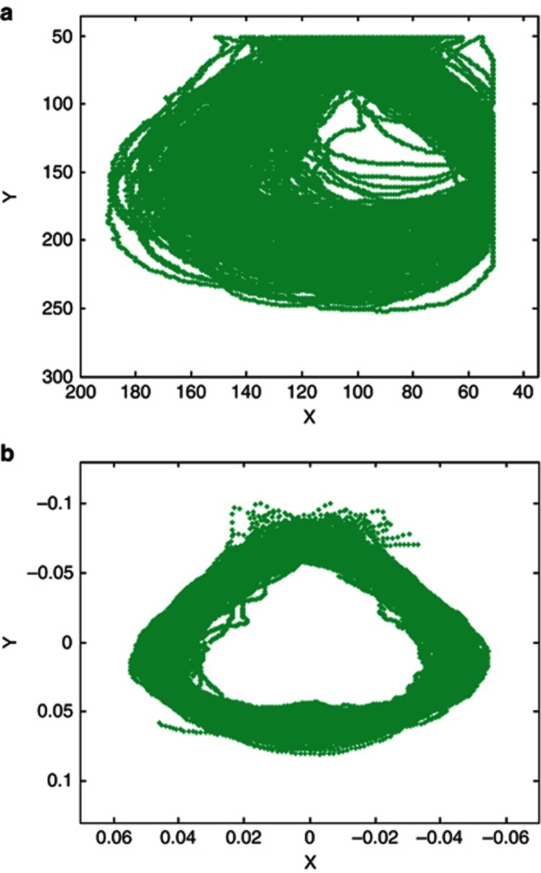
Leaf shape shows considerable variation caused by scale, rotation and translation (Figure 5a). Through alignment (see Materials and methods), all this has been filtered out from the objects (Figure 5b). A high dimension of leaf shape data described by RCC values, that is, the coordinates along the leaf boundaries, is reduced using PCA. It was found from PCA that six orthogonal axes, termed PCs, could explain 88.1% of the variation among the samples, which, ordered according to the percentages of variance they explained, are PC1, 47.3% PC2, 23.2% PC3, 6.7% PC4, 5.1% PC5, 3.5% and PC6, 2.3%. These PCs can describe each leaf shape by capturing different aspects of leaf shape variability including global and local.

Figure 5.

Linking 360 coordinates on the leaf outlines for leaves of all sampled trees from the mapping population. In (a), raw leaf shapes, showing variation in scale, position and orientation. In (b), this variation is removed from the objects through shape alignment.

To map the QTLs that affect leaf shape, the PC values were associated with 29 microsatellite markers. Table 1 tabulates the names of significant markers, their allele frequencies, the allele frequencies of the QTLs detected by these markers and marker-QTL LD. PC1, PC3, PC4 and PC5 were each found to exhibit significant associations with three markers, whereas PC6 is associated with one marker. Some markers may be associated with different types of PC axes, suggesting that the same QTLs have a pleiotropic effect on different features of a leaf shape. For example, marker GCPM_1063 is significantly associated with PC1 (P=1.01 × 10⁻¹⁰), PC3 (P=1.88 × 10⁻⁸), PC4 (P=1.14 × 10⁻⁷) and PC5 (P=3.55 × 10⁻⁷). It is possible that the same QTL causes the association of GCPM_1063 with these four PC axes because the QTLs detected for all the four PC axes have a similar allele frequency (0.49–0.51) and LD (0.09–0.12).

Table 1. Detection of leaf shape QTLs by the linkage disequilibrium analysis of microsatellite markers in a natural population of poplar.

PC (%explained)	Microsatellite marker	Effect, P-value	q	p	D	LD, P-value
PC1 (47.3)	GCPM_1063	1.01 × 10−10	0.74	0.49	0.12	1.77 × 10−15
	GCPM_1026-1	2.42 × 10−10	0.31	0.43	−0.12	2.42 × 10−13
	GCPM_1093-1	1.93 × 10−5	0.43	0.47	−0.05	1.57 × 10−3
PC3 (6.7%)	GCPM_1063	1.88 × 10−8	0.81	0.51	0.09	2.94 × 10−13
	GCPM_1064-1	1.68 × 10−5	0.44	0.43	−0.05	8.20 × 10−6
	GCPM_1-1	3.42 × 10−4	0.73	0.56	0.08	1.72 × 10−11
PC4 (5.1%)	GCPM_1063	1.14 × 10−7	0.77	0.51	0.13	0
	GCPM_1026-1	9.56 × 10−7	0.60	0.23	0.07	4.64 × 10−13
	GCPM_1034-1	8.54 × 10−4	0.45	0.14	−0.06	3.49 × 10−7
PC5 (3.5%)	GCPM_1063	3.55 × 10−7	0.79	0.51	0.10	0
	GCPM_1064-1	1.63 × 10−4	0.72	0.43	0.11	0
	GCPM_1025-1	4.95 × 10−4	0.73	0.44	0.11	0
PC6 (2.3%)	GCPM_1053-1	2.11 × 10−4	0.26	0.49	−0.12	0

Abbreviations: D, linkage disequilibrium between the marker and QTL; p, allele frequency of a marker; q, allele frequency of a QTL detected by the marker.

The effects of QTLs are tested by hypothesis (13), and the LD between markers and QTLs tested by hypothesis (14).

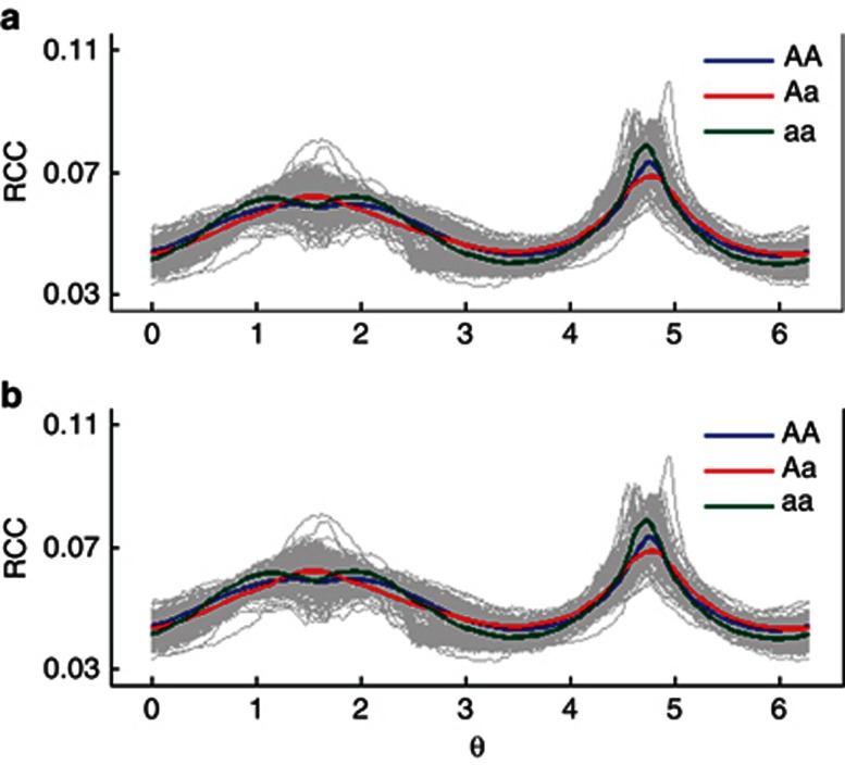
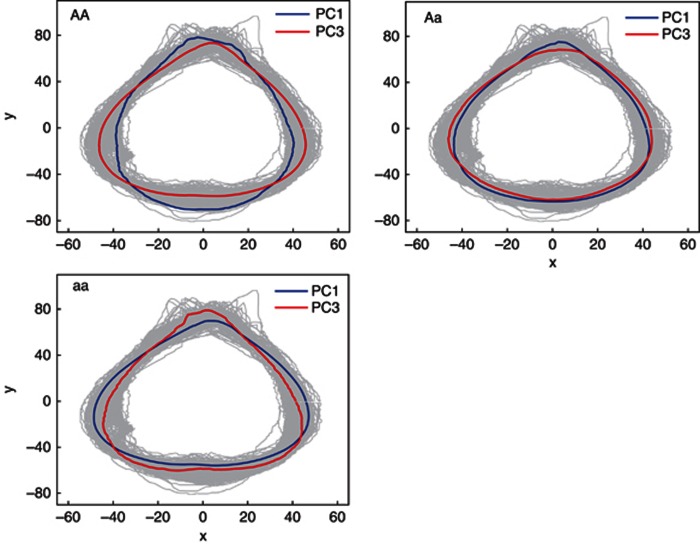
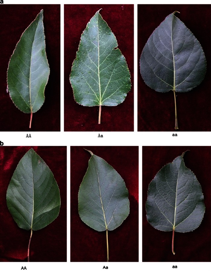
In general, the QTLs detected by PC1 control overall leaf shape variation, whereas the QTLs detected by the other PCs are responsible for local leaf variation. Figure 6 illustrates the fitness of PC1 curves (A) and PC3 curves (B) to the RCC curves of all poplar trees, respectively, for three genotypes, AA, Aa and aa, at the QTL detected by marker GCPM_1063. Difference in leaf shape explained by PC1 and PC3 curves of the same QTL genotype is diagrammed in Figure 7 where such a difference is found to be genotype-specific. Generally speaking, the QTL detected by marker GCPM_1063 alters leaf shape from lanceolate (AA) to ovate-orbicular (Aa) to ovate (aa) through PC1 (Figure 8a), whereas this QTL determines the detailed structure of broadly ovate leaf shape, for example, different degrees of deltoidness at leaf base among the three genotypes (Figure 8b).

Figure 6.

RCC curves of leaf shape as a function of radial angle θ at the centroid, explained by the PC1 curve (a) and PC3 curves (b) for the three genotypes, AA, Aa and aa, at the QTL detected by marker GCPM_1063.

Figure 7.

The pleiotropic control of the same QTL on different features of leaf shape specified by PC1 and PC2. The difference of leaf shape defined by PC1 (blue) and PC3 axes (red) for the same genotype, AA, Aa or aa, is shown.

Figure 8.

Three representative leaf shapes of P. szechuanica var. tibetica corresponding to three different genotypes, AA, Aa and aa, at the QTL detected by marker GCPM_1063. PC1 defines overall leaf shape (a), whereas PC3 defines local shape variability (b). In (b), three genotypes all have broadly ovate leaf shape, but genotypes AA and Aa are more deltoid than genotype aa at leaf base.

The LD of markers with the QTLs are highly significant (P=1.57 × 10⁻³−0), suggesting that these QTLs can possibly map to a narrow genomic region. Of the two other PC1 QTLs that control overall leaf shape in a similar manner, but with a lesser extent, one detected by marker GCPM_1026-1 displays a larger effect on shape variation and is also closer to the QTL than one detected by marker GCPM_1093-1 (Table 1). The QTLs associated with the other PCs tend to affect the local variation of leaf shape at various positions of leaves. Although it is subtle, such local variation may be tightly linked with gradient changes of some environmental factors. Thus, ecological functions of ‘local' QTLs deserve further investigations.

Discussion

Knowledge about the genetic mechanisms for shape variation has far-reaching implications for a range spectrum of scientific disciplines (Ricklefs and Miles, 1994; Klingenberg, 2010). Comparing the anatomical and shape feature of organisms has been a central element of biology for centuries (Bookstein, 1978; Klingenberg and Leamy, 2001; Monteiro et al., 2002; Adams et al., 2004). For example, as one of the most conspicuous aspects of a plant's phenotype, leaf shape has been used to provide an intricate link between biological structure and function in changing environments (Tsukaya, 2005). With an increasing interest in studying shape genetics (Weber et al., 1999; Langlade et al., 2005; Mezey et al., 2005; Leamy et al., 2008), we have now developed a computational model for mapping specific QTLs that contribute to shape variation by using leaf shape as an example of demonstration.

Unlike traditional morphological data that concern single measurements of an object, such as size or weight, shape data that capture the proportions and relative positions of various parts of the object are viewed as a photograph (Klingenberg, 2010). We incorporate statistical models for extracting shape information from photographs into a mixture-model framework for QTL mapping. Different aspects of a shape are specified by orthogonal PCs. Statistical parameters that define genotype-specific differences in shape-related PCs are estimated by implementing the EM algorithm. This so-called shape-mapping model enables geneticists to examine the control patterns of specific QTLs on the origin, properties and functions of leaf shape.

Our model is, to some extent, similar to the approaches for shape-QTL mapping by (Langlade et al., 2005 and Klingenberg 2003, 2010) in terms of the use of PCA to reduce data dimension. However, our model is distinct from the latter two types of shape modeling. First, rather than using a limited number of sparse anatomical landmarks, that is, those points, assigned by an expert, that corresponds between objects of study in a way meaningful in the disciplinary context, our model detects and capitalizes on mathematical landmarks that are located on an object according to its specific mathematical or geometrical property. In the examples shown in Figure 2, it is difficult to find anatomical landmarks at those outlines where leaf margins are abruptly lobed. This shape variation can be well described by mathematical landmarks. Second, our model expresses a series of coordinates taken on an object as a RCC curve (that is, a function of radial angle θ at the centroid). Thus, more powerful statistical approaches, such as longitudinal data analysis of RCC, can be incorporated into a QTL mapping framework, enhancing the biological relevance of shape mapping.

To demonstrate its application, shape mapping was used to map QTLs for leaf shape with the data collected from a natural population of P. szechuanica var. tibetica. This poplar species is naturally distributed in the mountains at an altitude of 1100−4600 m in southwestern China (Hamzeh and Dayanandan, 2004), providing an ideal model system to study the genetics of leaf morphology and its relationship with ecological adaptations. Interestingly, we detected a number of shape QTLs associated with microsatellite markers by shape mapping. From the PCA of shape data extracted from leaf images, six major PCs were detected to together explain 88.1% of the variation among leaf shapes. By mapping these PCs, we identified the QTLs that control leaf shape from various morphological aspects. Of these QTLs, those obtained through the major PC that account for almost a half of the variation determine the overall or global shape variation of leaves, whereas those through the other minor PCs control the local shape variation. It is worthwhile to further investigate specific QTLs that determine the ecological relationships of leaf shape and environmental factors by sampling more poplar trees from different populations.

Different from the work of Langlade et al. (2005), shape mapping focuses on mapping leaf shape by separating it from leaf size through uniformly scaling leaf images. Although this helps to clarify the genetic control of leaf shape in its own right, the biological functions of leaf size and shape may be inherently linked (Wang et al., 2010). Our model can be readily extended to perform simultaneous mapping of leaf shape and leaf size within a unifying framework, allowing the pleiotropic test of QTL effects on these two leaf traits. Also, given its critical role in trait control (Wang et al., 2010), epistasis between different QTLs should be modeled and tested by implementing multi-QTL genotypes into the mixture likelihood (1). With the availability of data collected for large-scale and complex problems in genetic, ecological and physiological research, our shape-mapping model described will provide a powerful analytical tool to effectively and efficiently test and build hypotheses, and extract useful information for scientific inferences and prediction.

Data archiving

There were no data to deposit.

The authors declare no conflict of interest

References

- Adams DC, Rohlf FJ, Slice DE. Geometric morphometrics: ten years of progress following the ‘revolution.'. Ital J Zool. 2004;71:5–16. [Google Scholar]
- Albertson RC, Streelman JT, Kocher TD, Yelick PC. Integration and evolution of the cichlid mandible: the molecular basis of alternate feeding strategies. Proc Natl Acad Sci USA. 2005;102:16287–16292. doi: 10.1073/pnas.0506649102. [DOI] [PMC free article] [PubMed] [Google Scholar]
- Belongie S, Malik J, Puzicha J. Shape matching and object recognition using shape contexts. IEEE Transac Pattern Anal Machine Intell. 2002;24:509–522. doi: 10.1109/TPAMI.2005.220. [DOI] [PubMed] [Google Scholar]
- Bookstein FL. The Measurement of Biological Shape and Shape Change. Springer-Verlag: New York, NY, USA; 1978. [Google Scholar]
- Churchill GA, Doerge RW. Empirical threshold values for quantitative trait mapping. Genetics. 1994;138:963–971. doi: 10.1093/genetics/138.3.963. [DOI] [PMC free article] [PubMed] [Google Scholar]
- Coen E, Rolland-Lagan A-G, Matthews M, Bangham JA, Prusinkiewicz P. The genetics of geometry. Proc Natl Acad Sci USA. 2004;101:4728–4735. doi: 10.1073/pnas.0306308101. [DOI] [PMC free article] [PubMed] [Google Scholar]
- Cootes TF, Taylor CJ, Cooper DH, Graham J. Active shape models—their training and application. Comput Vision Image Understand. 1995;61:38–59. [Google Scholar]
- Fu G, Berg A, Das K, Li J, Li R, Wu R. A statistical model for mapping morphological shape. Theor Biol Med Model. 2010;7:28. doi: 10.1186/1742-4682-7-28. [DOI] [PMC free article] [PubMed] [Google Scholar]
- Gilchrist AS, Crisafulli DCA. Using variation in wing shape to distinguish between wild and mass-reared individuals of Queensland fruit fly, Bactrocera tryoni. Entom Exp App. 2006;119:175–178. [Google Scholar]
- Gower JC, Dijksterhuis GB. Procrustes Problems. Oxford University Press: NY, USA; 2004. [Google Scholar]
- Hamzeh M, Dayanandan S. Phylogeny of Populus (Salicaceae) based on nucleotide sequences of chloroplast TRNT-TRNF region and nuclear rDNA. Am J Bot. 2004;91:1398–1408. doi: 10.3732/ajb.91.9.1398. [DOI] [PubMed] [Google Scholar]
- Kendall DG. Shape manifolds, procrustean metrics, and complex projective spaces. Bull London Math Soc. 1984;16:81–121. [Google Scholar]
- Kessler S, Sinha N. Shaping up: the genetic control of leaf shape. Curr Opin Plant Biol. 2004;7:65–72. doi: 10.1016/j.pbi.2003.11.002. [DOI] [PubMed] [Google Scholar]
- Klingenberg CP, Duttke S, Whelan S, Kim M. Developmental plasticity, morphological variation and evolvability: a multilevel analysis of morphometric integration in the shape of compound leaves. J Evol Biol. 2012;25:115–129. doi: 10.1111/j.1420-9101.2011.02410.x. [DOI] [PubMed] [Google Scholar]
- Klingenberg CP, Leamy LJ, Cheverud JM. Integration and modularity of quantitative trait locus effects on geometric shape in the mouse mandible. Genetics. 2004;166:1909–1921. doi: 10.1534/genetics.166.4.1909. [DOI] [PMC free article] [PubMed] [Google Scholar]
- Klingenberg CP, Leamy LJ, Routman EJ, Cheverud JM. Genetic architecture of mandible shape in mice: effects of quantitative trait loci analyzed by geometric morphometrics. Genetics. 2001;157:785–802. doi: 10.1093/genetics/157.2.785. [DOI] [PMC free article] [PubMed] [Google Scholar]
- Klingenberg CP, Leamy LJ. Quantitative genetics of geometric shape in the mouse mandible. Evolution. 2001;55:2342–2352. doi: 10.1111/j.0014-3820.2001.tb00747.x. [DOI] [PubMed] [Google Scholar]
- Klingenberg CP. Quantitative genetics of geometric shape: heritability and the pitfalls of the univariate approach. Evolution. 2003;57:191–195. doi: 10.1111/j.0014-3820.2003.tb00230.x. [DOI] [PubMed] [Google Scholar]
- Klingenberg CP. Evolution and development of shape: integrating quantitative approaches. Nat Rev Genet. 2010;11:623–635. doi: 10.1038/nrg2829. [DOI] [PubMed] [Google Scholar]
- Koenig D, Sinha N. Evolution of leaf shape: a pattern emerges. Curr Top Dev Biol. 2010;91:169–183. doi: 10.1016/S0070-2153(10)91006-5. [DOI] [PubMed] [Google Scholar]
- Lander ES, Botstein D. Mapping Mendelian factors underlying quantitative traits using RFLP linkage maps. Genetics. 1989;121:185–199. doi: 10.1093/genetics/121.1.185. [DOI] [PMC free article] [PubMed] [Google Scholar]
- Langlade NB, Feng X, Dransffeld T. Evolution through genetically controlled allometry space. Proc Natl Acad Sci USA. 2005;102:10221–10226. doi: 10.1073/pnas.0504210102. [DOI] [PMC free article] [PubMed] [Google Scholar]
- Leamy LJ, Klingenberg CP, Sherratt E, Wolf JB, Cheverud JM. A search for quantitative trait loci exhibiting imprinting effects on mouse mandible size and shape. Heredity. 2008;101:518–526. doi: 10.1038/hdy.2008.79. [DOI] [PubMed] [Google Scholar]
- Liang H, Mahadevan L. The shape of a long leaf. Proc Natl Acad Sci USA. 2009;106:22049–22054. doi: 10.1073/pnas.0911954106. [DOI] [PMC free article] [PubMed] [Google Scholar]
- Mezey JG, Houle D, Nuzhdin SV. Naturally segregating quantitative trait loci affecting wing shape of Drosophila melanogaster. Genetics. 2005;169:2101–2113. doi: 10.1534/genetics.104.036988. [DOI] [PMC free article] [PubMed] [Google Scholar]
- Mezey JG, Houle D. The dimensionality of genetic variation for wing shape in Drosophila melanogaster. Evolution. 2005;59:1027–1038. [PubMed] [Google Scholar]
- Monteiro LR, Diniz-Filho JA, dos Reis SF, Araújo ED. Geometric estimates of heritability in biological shape. Evolution. 2002;56:563–572. doi: 10.1554/0014-3820(2002)056[0563:GEOHIB]2.0.CO;2. [DOI] [PubMed] [Google Scholar]
- Nath U, Crawford BCW, Carpenter R, Coen E. Genetic control of surface curvature. Science. 2003;299:1404–1407. doi: 10.1126/science.1079354. [DOI] [PubMed] [Google Scholar]
- Ricklefs RE, Miles DB.1994Ecological and evolutionary inferences from morphology: an ecological perspectivein Wainwright PC, Reilly SM (eds.)Ecological Morphology University of Chicago Press: Chicago, IL, USA; 13–41. [Google Scholar]
- Rohlf FJ, Marcus LF. A revolution in morphometrics. Trends Ecol Evol. 1993;8:129–132. doi: 10.1016/0169-5347(93)90024-J. [DOI] [PubMed] [Google Scholar]
- Rolland-Lagan A-G, Bangham JA, Coen E. Growth dynamics underlying petal shape and asymmetry. Nature. 2003;422:161–163. doi: 10.1038/nature01443. [DOI] [PubMed] [Google Scholar]
- Rolland-Lagan A-G, Coen E, Impey SJ, Bangham JA. A computational method for inferring growth parameters and shape changes during development based on clonal analysis. J Theor Biol. 2005;232:157–177. doi: 10.1016/j.jtbi.2004.04.045. [DOI] [PubMed] [Google Scholar]
- Scarpella E, Barkoulas M, Tsiantis M. Control of leaf and vein development by auxin. Cold Spring Harb Perspect Biol. 2010;2:a001511. doi: 10.1101/cshperspect.a001511. [DOI] [PMC free article] [PubMed] [Google Scholar]
- Slice DE. Geometric morphometrics. Ann Rev Anthropol. 2007;36:261–281. [Google Scholar]
- Tanksley SD. The genetic, developmental, and molecular bases of fruit size and shape variation in tomato. Plant Cell. 2004;16:S181–S189. doi: 10.1105/tpc.018119. [DOI] [PMC free article] [PubMed] [Google Scholar]
- Tsukaya H. Leaf shape: genetic controls and environmental factors. Intl J Dev Biol. 2005;49:547–555. doi: 10.1387/ijdb.041921ht. [DOI] [PubMed] [Google Scholar]
- van der Knapp E, Lippman ZB, Tanksley SD. Extremely elongated tomato fruit controlled by four quantitative trait loci with epistatic interactions. Theor Appl Genet. 2002;104:241–247. doi: 10.1007/s00122-001-0776-1. [DOI] [PubMed] [Google Scholar]
- Wang Z, Liu T, Lin ZW, Hegarty J, Koltun WA, Wu R. A general model for multilocus epistatic interactions in case-control studies. PLoS One. 2010;5:e11384. doi: 10.1371/journal.pone.0011384. [DOI] [PMC free article] [PubMed] [Google Scholar]
- Wang ZH, Wu RL. A statistical model for high-resolution mapping of quantitative trait loci determining human HIV-1 dynamics. Stat Med. 2004;23:3033–3051. doi: 10.1002/sim.1870. [DOI] [PubMed] [Google Scholar]
- Weber K, Eisman R, Morey L, Patty A, Sparks J, Tausek M, et al. An analysis of polygenes affecting wing shape on chromosome 3 in Drosophila melanogaster. Genetics. 1999;153:773–786. doi: 10.1093/genetics/153.2.773. [DOI] [PMC free article] [PubMed] [Google Scholar]
- Wu R, Bradshaw HD, Stettler RF. Molecular genetics of growth and development in Populus. v. mapping quantitative trait loci affecting leaf variation. Am J Bot. 1997;84:143–153. [PubMed] [Google Scholar]