Perspective: Stochastic algorithms for chemical kinetics

Abstract

We outline our perspective on stochastic chemical kinetics, paying particular attention to numerical simulation algorithms. We first focus on dilute, well-mixed systems, whose description using ordinary differential equations has served as the basis for traditional chemical kinetics for the past 150 years. For such systems, we review the physical and mathematical rationale for a discrete-stochastic approach, and for the approximations that need to be made in order to regain the traditional continuous-deterministic description. We next take note of some of the more promising strategies for dealing stochastically with stiff systems, rare events, and sensitivity analysis. Finally, we review some recent efforts to adapt and extend the discrete-stochastic approach to systems that are not well-mixed. In that currently developing area, we focus mainly on the strategy of subdividing the system into well-mixed subvolumes, and then simulating diffusional transfers of reactant molecules between adjacent subvolumes together with chemical reactions inside the subvolumes.

INTRODUCTION

When Ludwig Wilhelmy, in 1850, described the buffered conversion of sucrose into glucose and fructose using a first-order ordinary differential equation (ODE),¹ ODEs were inaugurated as the standard tool for mathematically modeling chemical kinetics. The suitability of ODEs for that task must have seemed obvious to 19th century scientists: after all, ODEs provided the mathematical basis for that most fundamental of all dynamical theories, Newton's second law. But ODEs in chemical kinetics imply a continuous-deterministic time evolution for the species concentrations. That is at odds with the view, which was not universally accepted until the early 20th century, that matter consists of discrete molecules which move and chemically react in a largely random manner.

For a long time, scientists showed little concern with this mismatch. The first serious attempt to model the intrinsically discrete-stochastic behavior of a chemically reacting system was made in 1940 by pioneering biophysicist Max Delbrück;² however, no further work in that vein was done until the 1950s. An overview of work through the late 1960s has been given by McQuarrie.³ In the 1970s, procedures for stochastically simulating chemically reacting systems using large computers began to be devised. But controversies arose over the correct physical basis and mathematical formalism for stochastic chemical kinetics. By the end of the 1970s, that confusion, along with the fact that molecular discreteness and randomness posed no problems for ODEs in describing typical test-tube-size systems, effectively relegated stochastic chemical kinetics to a subject of only academic interest. That changed nearly two decades later, when Arkin, McAdams, and a growing number of other researchers^{4, 5, 6, 7} showed that in living cells, where reactant species are often present in relatively small molecular counts, discreteness and stochasticity can be important. Since then a great many papers have been published on the theory, computational methods, and applications of stochastic chemical kinetics, practically all aimed toward cellular chemistry.

In Sec. 2, we outline our perspective on the stochastic chemical kinetics of systems in which the reactant molecules are “dilute” and “well-mixed”—terms that will be defined shortly. The theoretical and computational picture for that relatively simple scenario has become greatly clarified over just the last dozen years. For situations where the reactant molecules crowd each other or are not well-mixed, situations that are quite common in cellular systems, progress has been made, but the going is slow. Many important questions have not yet been fully answered, and undoubtedly some have yet to be asked. In Sec. 3, we discuss some of the issues surrounding one major strategy for simulating systems that are not well-mixed. In Sec. 4 we briefly summarize recent accomplishments and current challenges.

DILUTE WELL-MIXED CHEMICAL SYSTEMS

The chemical master equation and the propensity function

It was primarily through the work of McQuarrie³ that what is now called the chemical master equation (CME) became widely known. For N chemical species S₁, …, S_N whose molecules can undergo M chemical reactions R₁, …, R_M, and with X_i(t) denoting the (integer) number of S_i molecules in the system at time t, the CME is a time-evolution equation for P(x, t|x₀, t₀), the probability that X(t) ≡ (X₁(t), …, X_N(t)) will be equal to x = (x₁, …, x_N), given that X(t₀) = x₀ for some t₀ ⩽ t:

$$\begin{array}{ccc}\hfill \frac{\partial P(\mathbf{x},t|{\mathbf{x}}_0,t_0)}{\partial t}& =& \sum _{j=1}^M[a_j(\mathbf{x}-{\mathit{\nu }}_j)P(\mathbf{x}-{\mathit{\nu }}_j,t|{\mathbf{x}}_0,t_0)\hfill \\ & & -a_j\left(\mathbf{x}\right)P(\mathbf{x},t|{\mathbf{x}}_0,t_0)].\hfill \end{array}$$ (1)

Here ν_j ≡ (ν_1j, …, ν_Nj), where ν_ij is the (signed integer) change in the S_i molecular population caused by one R_j event. And a_j, now called the propensity function for reaction R_j, is defined to be such that, for any infinitesimal time increment dt,

$$\begin{array}{ccc}\hfill a_j\left(\mathbf{x}\right)dt& \equiv & \mathrm{the}\mathrm{probability},\mathrm{given}\mathbf{X}\left(t\right)=\mathbf{x},\mathrm{that}\hfill \\ & & \mathrm{an}{R}_j\mathrm{event}\mathrm{will}\mathrm{occur}\mathrm{somewhere}\mathrm{inside}\hfill \\ & & \Omega \mathrm{in}[t,t+dt)(j=1,...,M).\hfill \end{array}$$ (2)

The CME 1 follows rigorously from this definition of a_j and the above definition of P via the laws of probability.

It is sometimes thought that the solution of the CME is a pristine probability function P(x, t) that describes the system independently of any observer-specified initial condition. That this is not so becomes clear when one realizes that if nothing is known about the state of the system at any time before t, then it will not be possible to say anything substantive about the state of the system at t. The solution P(x, t | x₀, t₀) of the CME 1 actually describes the gradually eroding knowledge that an observer, who last observed the system's state at time t₀, has of the state of the system as time increases beyond t₀.⁸

The key player in the CME 1 from the point of view of physics is the propensity function a_j defined in Eq. 2. As its name suggests, a_j quantifies how likely it is that reaction R_j will fire. Early work on the CME tended to view a_j as merely an ad hoc stochastic extension of the conventional reaction rate in the ODE formalism, with the latter having the more rigorous physical justification. But the situation is actually the other way around. As will become clear later in this section, the ODE formalism is an approximation of the stochastic formalism which is generally accurate only if the system is sufficiently large. Therefore, although there is a very close connection between propensity functions and conventional deterministic reaction rates, the latter, being an approximate special case of the former, cannot be used to derive the former. Nor can propensity functions be justifiably obtained by assuming hypothetical models or rules. An honest derivation of the propensity function must look directly to molecular physics to see how chemical reaction events actually occur, and then adopt a mathematical formalism that accurately characterizes that physical behavior.

Physical justification for the propensity function

The implicit assumption in 2 that a chemical reaction is a physical event that occurs practically instantaneously means that, at least for the dilute solution systems that we will be primarily concerned with here, every R_j must be one of two types: either unimolecular, in which a single molecule suddenly changes into something else; or bimolecular, in which two molecules collide and immediately change into something else. Trimolecular and reversible reactions in cellular chemistry nearly always occur as a series of two or more unimolecular or bimolecular reactions.

Unimolecular reactions of the form S₁ → ⋯ are inherently stochastic, usually for quantum mechanical reasons; there is no formula that tells us precisely when an S₁ molecule will so react. But it has been found that such an R_j is practically always well described by saying that the probability that a randomly chosen S₁ molecule will react in the next dt is equal to some constant c_j times dt. Summing c_jdt over all x₁S₁ molecules in Ω, in accordance with the addition law of probability, gives Eq. 2 with a_j(x) = c_jx₁.

The bimolecular reaction S₁ + S₂ → ⋯ is more challenging. In 1976, Gillespie^{9, 10} presented a simple kinetic theory argument showing that, if the reactant molecules comprise a well-mixed dilute gas inside Ω at temperature T, then a propensity function for S₁ + S₂ → ⋯ as defined in 2 exists and is given by

$$a_j(x_1,x_2)=\left(\pi {\sigma }_{12}^2{\overline{v}}_{12}{q}_j{\Omega }^{-1}\right)·x_1{x}_2(\mathrm{dilute}\mathrm{gas}).$$ (3a)

Here, σ₁₂ is the average distance between the centers of a pair of reactant molecules at collision (the sum of their radii for hard sphere molecules); ${\overline{v}}_{12}=\sqrt{\left(8k_{\mathrm{B}}T\right)/\left(\pi m_{12}\right)}$ is their average relative speed, with m₁₂ being their reduced mass; and q_j is the probability that an S₁-S₂ collision will produce an R_j reaction.¹¹

The derivation of Eq. 3a¹¹ is valid only if the reactant molecules are “well-mixed” and “dilute.” The well-mixed requirement means that a randomly selected reactant molecule should no more likely be found in any one subvolume of the system than in any other subvolume of the same size. But note this does not require that there be a perfectly regular placement of the reactant molecules inside Ω, nor that there be a large number of those molecules. If this well-mixed requirement cannot be sustained by the natural motion of the molecules, then it must be secured by external stirring. The dilute requirement means that the average separation between two reactant molecules should be very large compared to their diameters, or equivalently, that the total volume occluded by all the reactant molecules should comprise only a very small fraction of Ω.

Generalizing the dilute gas result 3a to a solution is obviously a necessary first step toward making the CME applicable to cellular chemistry. But doing that has long seemed problematic. According to the standard theory of diffusion, the root-mean-square displacement of a molecule in time Δt is proportional to $\sqrt{\Delta t}$; this suggests, at least on the basis of the way in which the dilute-gas result 3a is derived,¹¹ that the probability for a pair of diffusing molecules to react in the next dt might not have the linear dependence on dt demanded by 2. But in 2009, a detailed physics argument was produced¹² which shows that if the S₁ and S₂ molecules are solute molecules, well-mixed and dilute (in the above sense) in a bath of very many much smaller solvent molecules, then a propensity function for S₁ + S₂ → ⋯ as defined in 2 does exist, and is given explicitly by

$$\begin{array}{ccc}\hfill a_j(x_1,x_2)& =& \left(\frac{4\pi {\sigma }_{12}^2{D}_{12}{\overline{v}}_{12}{q}_j{\Omega }^{-1}}{4D_{12}+{\sigma }_{12}{\overline{v}}_{12}{q}_j}\right)·x_1{x}_2\hfill \\ & & \left(\mathrm{dilute}\mathrm{solution}\right).\hfill \end{array}$$ (3b)

Here, D₁₂ is the sum of the diffusion coefficients of the S₁ and S₂ molecules, and the other quantities are as previously defined. Note that the requirement for diluteness in this solution context applies only to the reactant solute molecules, and not to the solvent molecules. In the “fast-diffusion” limit defined by $4D_{12}\gg {\sigma }_{12}{\overline{v}}_{12}{q}_j$, Eq. 3b reduces to the dilute gas result 3a. At the opposite “diffusion limited” extreme $4D_{12}\ll {\sigma }_{12}{\overline{v}}_{12}{q}_j$, the factor in parentheses in Eq. 3b reduces to 4πσ₁₂D₁₂Ω⁻¹, which corresponds to a well known deterministic rate result that can be obtained by adapting Smoluchowski's famous analysis of colloidal coagulation.¹³ The derivation of Eq. 3b actually makes use of the Smoluchowski analysis, but does so in a way that takes account of the fact that the standard diffusion equation, on which the Smoluchowski analysis is based, is physically incorrect on small length scales.¹²

It remains to be seen how the propensity function hypothesis 2 will fare if the reactant molecules crowd each other, or if they move by active transport mechanisms along physically confined pathways. Even greater challenges attend relaxing the well-mixed assumption, because without it the “state” of the system can no longer be defined by only the total molecular populations of the reactant species. Those populations must be supplemented with information on the positions of the reactant molecules in order to advance the system in time. That in turn will require tracking the movement of individual molecules in a manner that is physically accurate yet computationally efficient—a very tall order! Some efforts in these directions will be discussed in Sec. 3. But here we will assume that the propensity function as defined in Eq. 2 exists, and further that it has the form c_jx₁ for the unimolecular reaction S₁ → ⋯, the form c_jx₁x₂ for the bimolecular reaction S₁ + S₂ → ⋯, and the form $c_j\frac{1}{2}{x}_1(x_1-1)$ for the bimolecular reaction 2S₁ → ⋯. Also important for later development of the theory is the fact that c_j will be independent of the system volume Ω for unimolecular reactions, and inversely proportional to Ω for bimolecular reactions. The latter property, which can be seen in both Eqs. 3a, 3b, reflects the obvious fact that it will be harder for two reactant molecules to find each other inside a larger volume.

The stochastic simulation algorithm

The difficulty of solving the CME for even very simple systems eventually prompted some investigators to consider the complementary approach of constructing simulated temporal trajectories or “realizations” of X(t). Averaging over sufficiently many such realizations can yield estimates of any average that is computable from the solution P(x, t | x₀, t₀) of the CME, and examining only a few realizations often yields insights that are not obvious from P(x, t | x₀, t₀). The earliest known constructions of simulated trajectories were made in 1972 by Nakanishi¹⁴ and Šolc and Horsák,¹⁵ and in 1974 by Bunker et al.¹⁶ But all these simulation procedures either were designed for specific simple systems, or else made heuristic approximations.

In 1976 Gillespie^{9, 10} proposed an exact, general-purpose procedure for simulating chemical reactions which is now called the stochastic simulation algorithm (SSA). The derivation of the SSA starts by posing the following question: Given the system's state X(t) = x at time t, at what time t + τ will the next reaction in the system occur, and which R_j will that next reaction be? Since, owing to the probabilistic nature of Eq. 2, τ and j must be random variables, the answer to this question can be supplied only by their joint probability density function (PDF), p(τ, j | x, t). That function is defined so that p(τ, j | x, t) · dτ gives the probability, given X(t) = x, that the next reaction event in the system will occur in the time interval $[t+\tau ,t+\tau +d\tau )$ and will be an R_j. Gillespie⁹ showed that Eq. 2 together with the laws of probability implies that this PDF is given by

$$p(\tau ,j|\mathbf{x},t)={\mathrm{e}}^{-a_0\left(\mathbf{x}\right)\tau }{a}_j\left(\mathbf{x}\right),$$ (4)

where $a_0\left(\mathbf{x}\right)\equiv {\sum }_{k=1}^M{a}_k\left(\mathbf{x}\right)$. The SSA is thus the following computational procedure:

1. In state x at time t, evaluate (as necessary) a₁(x), …, a_M(x), and their sum a₀(x).

2. Generate two random numbers τ and j according to the PDF 4.

3. Actualize the next reaction by replacing t ← t + τ and x ← x + ν_j.

4. Record (x, t). Return to Step 1, or else end the simulation.

Step 2 of the SSA can be implemented using any of several different exact methods, and Gillespie's paper⁹ presented two: the direct method, which follows from a straightforward application of the inversion Monte Carlo generating technique to the PDF 4;¹⁷ and the next reaction method, which despite its indirectness is equally exact. Of those two methods, the direct method is usually more efficient, and it goes as follows: Draw two unit-interval uniform random numbers u₁ and u₂, and take¹⁷

$$\tau =\frac{1}{a_0\left(\mathbf{x}\right)}\ln \left(\frac{1}{1-u_1}\right),$$ (5a)

$$\begin{array}{c}\hfill j=\mathrm{the}\mathrm{smallest}\mathrm{integer}\mathrm{satisfying}\sum _{k=1}^j{a}_k\left(\mathbf{x}\right)>u_2{a}_0\left(\mathbf{x}\right).\end{array}$$ (5b)

Other exact methods for implementing step 2 were subsequently developed by other workers, and they offer computational advantages in various specific situations. The most useful of those appear to be: the next reaction method of Gibson and Bruck,¹⁸ which is a major reformulation of the first reaction method; the first family method of Lok (described in Ref. 19); the optimized direct method of Cao et al.;²⁰ the sorting direct method of McCollum et al.;²¹ the modified next reaction method of Anderson,²² which in this context is the same as the next reaction method¹⁸ but is more flexibly couched in the “random time change representation” of Kurtz;^{23, 24} and the composition-rejection method of Slepoy et al.²⁵ An in-depth critique of the computational efficiencies of these and a few other methods has been given by Mauch and Stalzer.²⁶

Delayed events are difficult to incorporate analytically into the CME, but they can be handled easily by the SSA. Thus, suppose a reaction occurring at time t₁ signals that, independently of any subsequent reactions that might occur, an event E_d will occur at time t₁ + τ_d; e.g., a DNA transcription might start at time t₁ and produce an mRNA a time τ_d later. The event's delay time τ_d could either be a specified value, or it could be a random value that has been sampled from some known PDF. In either case, E_d and its time t₁ + τ_d are logged into a “delayed-event queue” which will temporarily halt the simulation when a reaction is first called for at some time t′ > t₁ + τ_d. Since such a call implies that nothing happens between the time of the last reaction event and t₁ + τ_d, the SSA simply advances the system without change to time t₁ + τ_d, discharges the event E_d, and then resumes the simulation from time t₁ + τ_d (ignoring the call for a reaction at time t′). Contingencies can also be easily accommodated; thus, if the delayed event E_d will occur at time t₁ + τ_d only if some other event E_c does not occur first, then if and when E_c occurs in [t₁, t₁ + τ_d] the SSA simply removes E_d from the queue.

Tau-leaping

It often happens that the average time between reactions, which can be shown from Eq. 4 to be $a_0^{-1}\left(\mathbf{x}\right)$, is so small that simulating every reaction event one at a time is not computationally feasible, no matter what method is chosen to implement step 2 of the SSA. Tau-leaping, introduced in 2001 by Gillespie,²⁷ aims to give up some of the exactness of the SSA in return for a gain in computational efficiency. It “leaps” the system ahead by a pre-selected time τ which may encompass more than one reaction event (this τ is not the same as the time τ to the next reaction in the SSA). The procedure for doing that is a straightforward consequence of the fact that the Poisson random variable with mean aτ, which we denote by $\mathcal{P}\left(a\tau \right)$, gives the (integer) number of events that will occur in the next time τ, provided that the probability of a single event occurring in any infinitesimal time dt is adt where a is any positive constant. Therefore, given X(t) = x, if τ chosen small enough that

$$\begin{array}{c}\hfill a_j\left(\mathbf{x}\right)\approx \mathrm{constant}\mathrm{in}[t,t+\tau ),\forall j\left(1\mathrm{st}\mathrm{leap}\mathrm{condition}\right),\end{array}$$ (6)

then during the interval [t, t + τ) there will be $\approx \mathcal{P}\left(a_j\left(\mathbf{x}\right)\tau \right)$ firings of reaction channel R_j. Since each of those firings augments the state by ν_j, the state at time t + τ will be²⁷

$$\mathbf{X}(t+\tau )\doteq \mathbf{x}+\sum _{j=1}^M{\mathcal{P}}_j\left(a_j\left(\mathbf{x}\right)\tau \right){\mathit{\nu }}_j,$$ (7)

where the ${\mathcal{P}}_j$ are M independent Poisson random variables. Equation 7 is called the tau-leaping formula. Its accuracy depends solely on how well condition 6 is satisfied.

Implementing tau-leaping at first seems straightforward: choose a value for τ, generate M Poisson random numbers with respective means a₁(x)τ, …, a_M(x)τ, and then evaluate Eq. 7. But in practice, there are problems. One is to determine in advance the largest value of τ that satisfies the leap condition 6. The strategy for doing that in Gillespie's original paper²⁷ was flawed, and allowed leaps to be taken that could produce substantial changes in propensity functions that have relatively small values. This not only produced inaccurate results, it also occasionally caused the population of some reactant species to go negative.²⁸ Another problem in implementing tau-leaping is that, while tau-leaping does become exact in the limit τ → 0, it also becomes infinitely inefficient in that limit: when τ is near zero, the M generated Poisson random numbers in Eq. 7 will usually all be zero, and that results in a computationally expensive leap with no change of state. A way is therefore needed to make tau-leaping segue to the SSA automatically and efficiently as τ becomes comparable to the average time $a_0^{-1}\left(\mathbf{x}\right)$ to the next reaction. A series of improvements in tau-leaping culminating in the 2006 paper of Cao et al.²⁹ solves these two problems for most practical applications. A tutorial presentation of that improved tau-leaping procedure is given in Ref. 30.

Among several variations that have been made on tau-leaping, three are especially noteworthy: the implicit tau-leaping method of Rathinam et al.,³¹ which adapts implicit Euler techniques developed for stiff ODEs to a stochastic setting; the R-leaping method of Auger et al.,³² which leaps by a pre-selected total number of reaction firings instead of by a pre-selected time; and the unbiased post-leap rejection procedure of Anderson.³³

Connection to the traditional ODE approach

Tau-leaping is also important because it is the first step in connecting the discrete-stochastic CME/SSA formalism with the continuous-deterministic ODE formalism. The second step along that path focuses on situations in which it is possible to choose a leap time τ that is not only small enough to satisfy the first leap condition 6, but also large enough to satisfy

$$a_j\left(\mathbf{x}\right)\tau \gg 1,\forall j\left(2\mathrm{nd}\mathrm{leap}\mathrm{condition}\right).$$ (8)

In that circumstance, we can exploit two well known results concerning $\mathcal{N}(\mu ,{\sigma }^2)$, the normal random variable with mean μ and variance σ²: First, when m ≫ 1, the Poisson random variable $\mathcal{P}\left(m\right)$ can be well approximated by $\mathcal{N}(m,m)$, at least for reasonably likely sample values of those two random variables. And second, $\mathcal{N}(\mu ,{\sigma }^2)\equiv \mu +\sigma \mathcal{N}(0,1)$. Applying those two results to the tau-leaping formula 7, again assuming that both leap conditions 6, 8 are satisfied, yields

$$\begin{array}{c}\hfill \mathbf{X}(t+\tau )\doteq \mathbf{x}+\sum _{j=1}^M{\mathit{\nu }}_j{a}_j\left(\mathbf{x}\right)\tau +\sum _{j=1}^M{\mathit{\nu }}_j\sqrt{a_j\left(\mathbf{x}\right)}{\mathcal{N}}_j(0,1)\sqrt{\tau }.\end{array}$$ (9a)

From one point of view, Eq. 9a is simply an approximation of the tau-leaping formula 7 that has replaced Poisson random numbers with normal random numbers. But recalling that x ≡ X(t), and noting that because of condition 6 we can regard τ as an infinitesimal dt on macroscopic time scales, we can also write Eq. 9a as

$$\begin{array}{ccc}\hfill \mathbf{X}(t+dt)-\mathbf{X}\left(t\right)& \doteq & \sum _{j=1}^M{\mathit{\nu }}_j{a}_j\left(\mathbf{X}\left(t\right)\right)dt\hfill \\ & & +\sum _{j=1}^M{\mathit{\nu }}_j\sqrt{a_j\left(\mathbf{X}\left(t\right)\right)}{\mathcal{N}}_j(0,1)\sqrt{dt}.\hfill \end{array}$$ (9b)

This equation has the canonical form of a “stochastic differential equation” or “Langevin equation.”³⁴ It is called the chemical Langevin equation (CLE).

This derivation of the CLE is due to Gillespie.³⁵ For reasons that can be understood from this derivation, the CLE will not accurately describe “rare events.”³⁶ But if the system admits a dt ≡ τ that is small enough to satisfy the first leap condition 6 yet also large enough to satisfy the second leap condition 8, then the CLE should give a fair account of the typical (as opposed to the atypical) behavior of the system. As a set of N coupled equations, the CLE 9b is much less formidable than the CME 1, since the latter is a set of coupled equations indexed by x. Furthermore, since a numerical simulation using Eq. 9a will, as a consequence of condition 8, step over very many reaction events for each reaction channel, the CLE will be much faster than the SSA.

But the CLE requires both leap conditions to be satisfied, and that is not a trivial requirement since it is easy to find systems for which that cannot be done. But in 2009, Gillespie³⁷ proved that both leap conditions can always be satisfied, and hence the CLE will always be valid, if the system is made sufficiently “large” in the sense of the thermodynamic limit—where the molecular populations are imagined to go to infinity along with the system volume Ω while the concentrations remain constant. The proof of that result uses the earlier noted fact that real-world elemental reactions R_j have propensity functions that are either of the form c_jx_i with c_j independent of Ω, or c_jx_ix_k with c_j proportional to Ω⁻¹; that implies that, in the thermodynamic limit, all real-world propensity functions a_j(x) grow linearly with the system size. Therefore, roughly speaking, after satisfying the first leap condition 6 by fixing τ sufficiently small, we can satisfy the second leap condition 8 simply by taking the system sufficiently close to the thermodynamic limit.

As the thermodynamic limit is approached, the left side of the CLE 9b grows linearly with the system size; the first term on the right, being proportional to the propensity functions, also grows linearly with the system size; and the second term on the right, being proportional to the square roots of the propensity functions, grows like the square root of the system size. So in the full thermodynamic limit, the second term on the right of the CLE 9b becomes negligibly small in comparison with the other terms, and that equation reduces to the ODE³⁸

$$\frac{d\mathbf{X}\left(t\right)}{dt}\doteq \sum _{j=1}^M{\mathit{\nu }}_j{a}_j\left(\mathbf{X}\left(t\right)\right).$$ (10a)

This is the reaction rate equation (RRE), the ODE of traditional chemical kinetics. Since as we have just seen, the RRE is generally valid only in the thermodynamic limit, it is more commonly written in terms of the concentration variable³⁹Z(t) ≡ X(t)/Ω and the functions ${\tilde{a}}_j\left(\mathbf{z}\right)$, the latter being defined as the thermodynamic limit of ${\Omega }^{-1}{a}_j\left(\mathbf{x}\right)$:

$$\frac{d\mathbf{Z}\left(t\right)}{dt}\doteq \sum _{j=1}^M{\mathit{\nu }}_j{\tilde{a}}_j\left(\mathbf{Z}\left(t\right)\right).$$ (10b)

The convergence of the jump Markov process described by the CME 1 first to the continuous Markov process described by the CLE 9b and then in the thermodynamic limit to the ODE 10b, also follows from results of Kurtz⁴⁰ on the approximation of density-dependent Markov chains.

The theoretical structure presented above is summarized in Fig. 1. As we proceed from the top of that figure to the bottom, we move toward approximations that require increasingly larger molecular populations, but are computationally more efficient. The question naturally arises: how many molecules must a system have in order to be reliably described at a particular level in Fig. 1? No general answer to that question can be given, since any answer will depend on the structure and the parameter values of the reaction network.

Figure 1.

Stochastic chemical kinetics is premised on the definition 2 of the propensity function in the top box, a definition which must look to molecular physics for its justification. The two solid-outlined boxes in yellow denote mathematically exact consequences of that definition: the chemical master equation 1 and the stochastic simulation algorithm 4. Dashed-outlined boxes denote approximate consequences: tau-leaping 7, the chemical Langevin equation 9, the chemical Fokker-Planck equation (not discussed here but see Ref. 35), and the reaction rate equation 10. The bracketed condition by each dashed inference arrow is the condition enabling that approximation: reading from top to bottom, those conditions are the first leap condition, the second leap condition, and the thermodynamic limit. The rationale for viewing the linear noise approximation (LNA)⁴¹ as an intermediate result between the CLE and the RRE is detailed in Ref. 42. It has been shown³⁷, ⁴² that for realistic propensity functions, getting “close enough” to the thermodynamic limit will ensure simultaneous satisfaction of the first and second leap conditions, at least for finite spans of time; therefore, the top-to-bottom progression indicated in the figure will inevitably occur as the molecular populations and the system volume become larger. But a given chemical system might be such that the largest value of τ that satisfies the first leap condition will not be large enough to satisfy the second leap condition; in that case, there will be no accurate description of the system below the discrete-stochastic level in the figure.

But it turns out that this question can be rendered practically irrelevant when doing simulations. To see why, suppose we have a tau-leaping implementation that efficiently segues to the SSA, such as the one described in Ref. 29, and using it we have found a τ that satisfies the first leap condition 6. Then the number of firings in the next τ of each reaction channel R_j will be well approximated by a Poisson random variable with mean a_j(x)τ, as in the tau-leaping formula 7. However, the call to the Poisson random number generator for a sample value of each ${\mathcal{P}}_j\left(a_j\left(\mathbf{x}\right)\tau \right)$ can be handled on a reaction-by-reaction basis: If a_j(x)τ is “large” compared to 1 then the Poisson random number generator can return instead a normal random number with mean and variance a_j(x)τ, as would happen for all R_j if we were using the Langevin leaping formula 9a. Or, if a_j(x)τ is “very large” compared to 1, so that the standard deviation $\sqrt{a_j\left(\mathbf{x}\right)\tau }$ is negligibly small compared to the mean a_j(x)τ, then the Poisson random number generator can return the non-random number a_j(x)τ, as would happen for all R_j if we were using the RRE 10a. In this way, each reaction channel R_j gets assigned to its computationally most efficient level in Fig. 1. It is not necessary for all the reactions channels to be assigned to the same level, nor even for the simulator to be aware of the level to which each reaction has been assigned.

The relationships outlined in Fig. 1 do not assume the applicability of the system-size expansion of van Kampen.⁴¹ But Wallace et al.⁴² have shown that the most commonly used result of the system-size expansion, namely, van Kampen's linear noise approximation (LNA),⁴¹ does have a place in Fig. 1: A surprisingly easy derivation⁴² of the LNA as a linearized approximation of the CLE 9b positions the LNA midway between the CLE and the RRE. That positioning is consistent with findings of Grima et al.⁴³ which indicate that the CLE is indeed more accurate than the LNA. The LNA describes the “initial departure” of the CLE from the deterministic RRE as we back away from the thermodynamic limit to a large but finite system. That initial departure is the appearance of normal fluctuations about the deterministic RRE solution, the variances of which are given explicitly by the LNA.

Concern about the accuracy of the CLE 9b prompts the question: Is there a formula for X(t + dt) − X(t) that is exactly equivalent to the CME/SSA? The answer is yes. It is the τ = dt version of the tau-leaping formula 7, which with x = X(t) reads

$$\mathbf{X}(t+dt)-\mathbf{X}\left(t\right)=\sum _{j=1}^M{\mathcal{P}}_j\left(a_j\left(\mathbf{X}\left(t\right)\right)dt\right){\mathit{\nu }}_j.$$

This is so because the only constraint on the accuracy of Eq. 7 is that τ be “small enough,” and that constraint is always satisfied by a true infinitesimal dt (the dt in the CLE is a “macroscopic” infinitesimal). However, this equation is practically useless for computation: since the Poisson random variable $\mathcal{P}\left(m\right)$ takes only integer values, then $\mathcal{P}\left(adt\right)$ for any finite a will almost always take the value 0, so the right side of the above equation will almost always be exactly 0. In contrast, the right side of the CLE 9b will almost always give some small but non-zero value for X(t + dt) − X(t). However, integrating the above equation from t₀ to t yields a more useful result:

$$\begin{array}{ccc}\hfill \mathbf{X}\left(t\right)-\mathbf{X}\left(t_0\right)& =& \sum _{j=1}^M{\int }_{t_0}^t{\mathcal{P}}_j\left(a_j\left(\mathbf{X}\left(t^{\prime }\right)\right)d{t}^{\prime }\right){\mathit{\nu }}_j\hfill \\ & =& \sum _{j=1}^M{Y}_j\left({\int }_{t_0}^t{a}_j\left(\mathbf{X}\left(t^{\prime }\right)\right)d{t}^{\prime }\right){\mathit{\nu }}_j,\hfill \end{array}$$ (11)

where the Y_j are “scaled, independent, unit-rate Poisson processes.”⁴⁴ Equation 11 is the random time change representation of Kurtz;^{23, 24} it is fully equivalent to the CME, in essentially the same way that a Langevin equation is fully equivalent to a Fokker-Planck equation. As shown by Anderson,²² Eq. 11 provides an alternate way of viewing the next reaction method of Gibson and Bruck;¹⁸ furthermore, it is the basis for Anderson's modified next reaction method²² and post-leap rejection tau-leaping procedure.³³

Stiff systems and the slow-scale SSA

Many real-world chemical systems include a mixture of fast and slow reaction channels which share one or more species. Perhaps the simplest example is

$$S_1\underset{c_2}{\overset{c_1}{\rightleftarrows }}{S}_2\stackrel{c_3}{\to }{S}_3\mathrm{with}{c}_2\gg c_3.$$ (12)

Here, successive R₃ firings will be separated by very many relatively uninteresting R₁ and R₂ firings; yet the latter will consume most of the time in a regular SSA run. This inefficiency cannot be overcome by ordinary tau-leaping, because leap times that satisfy the first leap condition will typically be on the order of the average time between the fastest reactions. An analogous computational inefficiency plagues deterministic chemical kinetics, where it is known as “stiffness.”

The slow-scale stochastic simulation algorithm (ssSSA)⁴⁵ is a way of handling this problem that combines efficacy with a clear theoretical justification. It begins by defining as “fast reactions” those which occur much more frequently than all the other reactions, which are designated “slow.” In reactions 12, that criterion designates R₁ and R₂ as fast reactions, and R₃ as a slow reaction.⁴⁶ Next the ssSSA identifies as “fast species” all those whose populations get changed by a fast reaction, and all the other species as “slow.” In reactions 12, S₁ and S₂ are fast species, and S₃ is a slow species. The ssSSA then defines the “virtual fast process” (VFP) to be the fast species populations evolving under only the fast reactions; in reactions 12, the VFP is X₁ and X₂ evolving under R₁ and R₂. Unlike the real fast process, where fast species populations can also get changed by slow reactions (in this case R₃), the VFP will always have a Markovian master equation. For the ssSSA to be applicable, the solution of the VFP master equation must have an asymptotic (t → ∞) steady-state which is effectively reached in a time that is small compared to the average time between slow reactions. In contrast to several other approaches to the stochastic stiffness problem (implicit tau-leaping, hybrid methods, etc.), the ssSSA does not require the fast species to have large molecular populations.

The goal of the ssSSA is to skip over uninteresting fast reactions and simulate only the slow ones, using modified versions of their propensity functions. What allows that to be done in a provably accurate manner is a result called the slow-scale approximation lemma.⁴⁵ It says that, under the conditions described above, replacing the slow reaction propensity functions with their averages over the fast species, as computed from the asymptotic VFP, will yield a set of modified propensity functions for the slow reactions that can be used in the SSA to simulate the evolution of the slow-species populations.

If the separation between the fast and slow timescales is sufficiently large, a substantial increase in simulation speed can usually be achieved with the ssSSA. The main challenge in implementing it is computing the required averages with respect to the asymptotic VFP. That can be done exactly for reactions 12, but approximations are usually required for more complicated reaction sets.⁴⁵ Often solutions of the equilibrium RRE corresponding to the asymptotic VFP will suffice,⁴⁷ although more sophisticated moment closure approximations for the asymptotic VFP will usually be more accurate.^{48, 49} In some circumstances it may be easier to estimate the required averages by making brief SSA runs of the VFP.⁵⁰ A software implementation of the ssSSA which automatically and adaptively partitions the system and efficiently computes the modified slow propensity functions for general mass action models is available.⁵¹

Rare events

In biochemical systems, rare events are important because their occurrence can have major consequences. But the standard SSA is ill-suited to quantifying rare events, since witnessing just one will, by definition, require an impractically long simulation run. A promising way around this difficulty called the weighted SSA (wSSA) was introduced in 2008 by Kuwahara and Mura.⁵² Instead of pursuing a traditional mean first passage time, they innovatively focused on the probability p(x₀, E; t) that the system, starting at time 0 in a specified state x₀, will first reach any state in a specified set E before a specified time t > 0. In other words, instead of trying to estimate the very long time it would take for the rare event to happen, the wSSA tries to estimate the very small probability that the rare event will happen in a time t of practical interest.

To compute p(x₀, E; t), the wSSA employs a Monte Carlo procedure called importance sampling. More specifically, it uses the SSA to advance the system to the target time t with the direct method 5, except that in the j-selection procedure 5b the propensity functions a_j(x) are replaced with a modified set of propensity functions b_j(x) which are biased toward the target states E. Correction for that bias is achieved by weighting the resulting realization by a product of the weights (a_j/a₀)/(b_j/b₀) for each reaction in the realization. Realizations that fail to reach E by time t are assigned a weight of 0. The average of these weighted realizations then estimates the probability p(x₀, E; t). Kuwahara and Mura⁵² showed that, with appropriate weighting, their wSSA can achieve substantial improvements over runs made using the unweighted SSA. Gillespie et al.⁵³ later introduced some refinements and clarifications, notably computing also the variance of the weighted trajectories, which quantifies the uncertainty in the estimate of p(x₀, E; t) and helps in finding optimally biased propensities.

Choosing the biased propensity functions is the major challenge of the wSSA, because it is often not clear which reactions should be biased nor how strongly, and making suboptimal choices can result in being even less efficient than the SSA. The original biasing scheme proposed by Kuwahara and Mura⁵² took $b_j\left(\mathbf{x}\right)={\gamma }_j{a}_j\left(\mathbf{x}\right)$, with the constants γ_j being chosen by intuition and trial-and-error. Subsequent innovations by Roh and Daigle and their collaborators^{54, 55, 56} have yielded a greatly improved version of the wSSA called the state-dependent doubly weighted SSA (sdwSSA). The sdwSSA: (i) allows the proportionality constants γ_j to be state dependent; (ii) biases not only the j-selection procedure but also the τ-selection procedure, replacing a₀(x) in 5a with b₀(x); and (iii) uses the multi-level cross-entropy method of Rubinstein⁵⁷ to develop a robust variance-estimation procedure that automatically determines the optimal biasing propensities b_j(x) with minimal input from the user.⁵⁶

Sensitivity analysis

A commonly used measure of the sensitivity of the average of some function f of state x (e.g., the molecular population of a particular species) to a parameter c (e.g., the rate constant of a particular reaction) at a specified time t > 0 given X(0) = x₀ is the change in that average when c is changed by some small amount ɛ, divided by ɛ:

$$\mathrm{sens}\left\{f(t;{\mathbf{x}}_0,c),\varepsilon \right\}\equiv \frac{⟨f(t;{\mathbf{x}}_0,c+\varepsilon )⟩-⟨f(t;{\mathbf{x}}_0,c)⟩}{\varepsilon }.$$

The most obvious way to estimate this quantity would be to use a finite difference approximation, i.e., make two independent sets of SSA runs to time t, one set using the parameter value c and the other using the parameter value c + ɛ, and compute the two averages ⟨f (t; x₀, c)⟩ and ⟨f (t; x₀, c + ɛ)⟩. But since ɛ needs to be small to localize the sensitivity at c, the difference between those two averages will usually be much smaller than the statistical uncertainties in their estimates for runs of reasonable length. As a consequence, the relative uncertainty in the estimate of the numerator on the right will usually be too large to be informative.

One way of dealing with this problem, the origin of which dates from the early days of Monte Carlo work, is called the common random numbers (CRN) procedure. It generates the SSA trajectories for c and c + ɛ in pairs, using the same uniform random number string {u_i} for each pair member, and then computes the average of the difference [f (t, c + ɛ) − f (t, c)] over the paired trajectories. The positive correlation between the paired trajectories caused by using the same string of random numbers to generate them gives [f (t, c + ɛ) − f (t, c)] a smaller variance about its average ⟨f (t, c + ɛ) − f (t, c)⟩ ≡ ⟨f (t, c + ɛ)⟩ − ⟨f (t, c)⟩ than in the independent run case. That in turn yields a more accurate estimate of the sensitivity for a given number of runs. But unless t is very small, the paired trajectories eventually get out of sync with each other. When that happens the correlation gradually dies off, and the CRN estimate of sens{(f (t; x₀, c), ɛ)} eventually becomes no more accurate than what would be obtained with the independent trajectories approach.

Rathinam et al.⁵⁸ have developed a significant improvement in this procedure called the common reaction path (CRP) method. In generating the paired c and c + ɛ trajectories, they use a variation of Anderson's modified next reaction method, in which paired trajectories use the same streams of unit exponential random number for each of the unit-rate Poisson processes Y_j (j = 1, …, M) in the random time change representation 11. That results in a significantly tighter correlation between paired trajectories than in the CRN procedure, and hence a significantly more accurate estimation of sens{(f (t; x₀, c), ɛ)} for the same computational effort. Anderson⁵⁹ has introduced a different variation of the modified next reaction method, called the coupled finite difference (CFD) procedure. It exploits the additivity of the Y_js in Eq. 11 to split them into sub-processes that are shared by paired trajectories in a way that usually gives even tighter and longer lasting correlations, and thus an even more accurate estimate of the sensitivity. References 58, 59 give detailed descriptions of the CRP and CFD sensitivity estimation procedures.

BEYOND WELL-MIXED SYSTEMS

Many situations require relaxing the assumption of a well-mixed reaction volume. Compartmentalization and localization of reactions to cellular membranes are ubiquitous mechanisms for cellular regulation and control. Even in cases where the geometry does not call for spatial resolution, short-range correlations can give rise to effects that can only be captured in simulations with spatial resolution.⁶⁰ And models increasingly call not only for spatial resolution, but also stochasticity.^{61, 62, 63, 64} A striking example of that is the oscillation of Min proteins in the bacterium E. coli, where a deterministic partial differential equation model could replicate wild type behavior but not the behavior of known mutants.⁶⁵

The reaction-diffusion master equation and simulation algorithm

A popular extension of the CME 1 to the spatially inhomogeneous case, which dates back at least to the 1970s,⁶⁶ is the reaction-diffusion master equation (RDME). The original idea of the RDME was to subdivide the system volume Ω into K uniform cubic subvolumes or “voxels” Ω_k (k = 1, …, K), each of edge length h, in such a way that within each voxel the reactant molecules can be considered to be well-mixed. Chemical reactions are then regarded as occurring completely inside individual voxels. The M nominal reactions {R_j} thus get replaced by KM reactions {R_jk}, where R_jk is reaction R_j inside voxel Ω_k. The propensity function a_jk for R_jk is the propensity function a_j for R_j, but now referred to the voxel volume |Ω_k| = h³, and regarded as a function of x_k = (x_1k, …, x_Nk) where x_ik is the current number of S_i molecules in Ω_k. The state-change vector ν_jk for R_jk is the ν_j for R_j, but confined to the space of x_k.

The diffusion of an S_i solute molecule in a sea of many smaller solvent molecules is generally assumed to be governed by the Einstein diffusion equation,

$$\frac{\partial p(\mathbf{r},t)}{\partial t}=D_i{\nabla }_{\mathbf{r}}^{2}p(\mathbf{r},t),$$ (13)

where p is the position PDF of the S_i molecule and D_i is its diffusion coefficient. But the RDME actually models the diffusion of an S_i molecule from voxel Ω_k to adjacent voxel Ω_l as a “diffusive transfer reaction” $R_{ikl}^{\mathrm{d}}$, whose propensity function $a_{ikl}^{\mathrm{d}}$ is d_iklx_ik where d_ikl is a constant, and whose state-change vector ${\mathit{\nu }}_{ikl}^{\mathrm{d}}$ decreases x_ik by 1 and increases x_il by 1. A variety of arguments show^{67, 68} that this modeling of the diffusive transfer of an S_i molecule to an adjacent voxel will, for sufficiently small h, approximate the behavior dictated by Eq. 13 provided the constant d_ikl is taken to be

$$d_{ikl}=\frac{D_i}{h^2}.$$ (14)

If B is the total number of planar surface boundary elements shared by two adjacent voxels, then there will be a total of 2NB diffusive transfer reactions.

Since diffusion is here being modeled as sudden jumps in the system's state of the same mathematical type as the dynamics of the state jumps induced by chemical reactions, the RDME is just the well-mixed CME 1 with the following reinterpretation of its symbols: the N-dimensional state vector x = {x_i} in Eq. 1 is now regarded as the KN-dimensional state vector {x_ik}; and the M propensity functions {a_j} and their associated state-change vectors {ν_j} in Eq. 1 are now regarded as those for the KM chemical reactions {R_jk} and the 2NB diffusive transfer reactions $\left\{R_{ikl}^{\mathrm{d}}\right\}$, with all of those reactions being treated on an equal footing. The algorithm for exactly simulating the system described by the RDME is therefore the SSA described in Sec. 2C, but with these same reinterpretations of x, a_j, and ν_j.

Uniform Cartesian meshes are attractive and efficient to use for relatively simple geometries, such as those that can be logically mapped to rectangles. For cellular geometries with curved inner and outer boundaries or subcellular structures, however, it is challenging to impose a Cartesian grid that respects the boundaries without a very fine mesh resolution. Using other types of meshes and discretizations, complex geometries can be accommodated in RDME simulations. By defining the jump probability rate constants on a general mesh based on a numerical discretization of Eq. 13, the probability to find a (mesoscopic) molecule inside a certain voxel at a given time will approximate that of a Brownian particle. Also, in the thermodynamic limit, the mean value of the concentration of the molecules in a voxel will converge to the solution of the classical (macroscopic) diffusion equation. The latter follows from classical results of Kurtz.⁶⁹

Isaacson and Peskin proposed to discretize the domain with a uniform Cartesian mesh but allowed for a general, curved boundary by using an embedded, or cut-cell, boundary method.^{70, 71} Engblom et al.⁷² took another approach, and used an unstructured triangular or tetrahedral mesh and a finite element method to discretize the domain and to compute the rate constants. The use of unstructured meshes greatly simplifies resolution of curved boundaries, but also introduces additional numerical considerations. Mesh quality becomes an important factor for how accurately the jump constants d_ikl can be computed. An in-depth discussion of the criteria imposed on the unstructured mesh and the discretization scheme can be found in Engblom et al.⁷² In Drawert et al.⁷³ the benefits and drawbacks of structured Cartesian versus unstructured triangular and tetrahedral meshes are further illustrated from a software and simulation perspective. Figure 2 shows parts of a Cartesian mesh (a) and a triangular mesh (b) in 2D. For the unstructured triangular mesh, molecules are assumed to be well-mixed in the “dual” elements, which are shown in pink. The same interpretation holds for a Cartesian mesh, where the dual is the staggered grid with respect to the primal mesh.

Figure 2.

Parts of a Cartesian mesh (a) and an unstructured triangular mesh (b). Molecules are assumed to be well-mixed in the local volumes that make up the dual elements of the mesh (depicted in pink color). For the Cartesian grid (a), the dual is simply the staggered grid. The dual of the triangular mesh in (b) is obtained by connecting the midpoints of the edges and the centroids of the triangles. (c) shows how a model of a eukaryotic cell with a nucleus (green) can be discretized with a mesh made up of triangles and tetrahedra. The figure is adapted from Ref. 70, where a model of nuclear import was simulated on this domain using the URDME software.

Perhaps the most challenging aspect of a RDME simulation today is to choose the mesh resolution. Common practice to decide whether a given mesh is appropriate is to repeat simulations with both coarser and finer meshes to determine whether the solution seems to change significantly with respect to some output of interest. Such a trial and error approach is not a satisfactory solution, since it is both time consuming and difficult to determine to what extent the accuracy of realizations of the stochastic process changes. Development of both a priori and a posteriori error estimates for the effects of discretization errors in a general reaction-diffusion simulation would help make RDME simulations more robust from the perspective of non-expert users, and make possible, e.g., adaptive mesh refinement. One step in this direction has been taken by Kang et al.⁷⁴ The situation is complicated by the fact that the standard formulation of the RDME breaks down for very small voxel sizes. This issue will be discussed in more detail in Sec. 3C.

Algorithms for spatial stochastic simulation

Variations on the several methods for implementing step 2 of the SSA in Sec. 2C have been developed for reaction-diffusion systems that exploit the relatively sparse dependencies among the reactions and/or the simple linear form of the diffusive transfer propensity functions. Since the total number of reactions (chemical plus diffusive transfer) will be very large if there are many voxels, the direct method⁹ will usually be very inefficient, because of the linear computational complexity of its j-selection step 5b in the number of voxels. Elf and Ehrenberg⁶² proposed the next subvolume method, which combines ideas of Lok's first family method (described in Ref. 19) and Gibson and Bruck's next reaction method,¹⁸ in an algorithm specifically tailored for reaction-diffusion systems. Reactions are grouped into families according to their voxels, and one samples first the firing time of the next voxel family, then whether it was a chemical reaction or a diffusive transfer reaction, and finally which particular reaction. The methodology of the next reaction method is used to select the next firing voxel, so the complexity in selecting the next event increases only logarithmically with the number of voxels.

As the voxel size h is made smaller, the growing number of voxel boundaries together with the increasing values of d_ikl in Eq. 14 conspire to increase the number of diffusive transfer events that occur over a fixed interval of system time. This is illustrated in Table 1, where we show the execution time for next subvolume method as implemented using the URDME software package,⁷² when applied to a 3D simulation of Min oscillations in the rod-shaped bacterium E. coli.⁶⁵ Although the time to generate each individual event (fourth column) scales well with the number of voxels (second column), the total time to simulate the system (third column) grows rapidly. For the finest mesh resolution, 99.98% of all events are diffusive transfers. Thus, the stochastic simulation of reaction-diffusion systems with ever finer spatial resolution eventually becomes dominated by transfers of individual molecules between adjacent voxels. This will be so whether or not the reactions are diffusion-limited. Algorithm development to increase the speed of simulations of reaction-diffusion systems has therefore focused on ways to reduce the cost of diffusive transfers through approximations that aggregate the diffusion events in order to update the system's state.

Table 1.

Simulation times for a spatial stochastic system simulated to a final time of 200 s with the next-subvolume method, as implemented in URDME.

hmax1	No. of voxels	t (s)2	No. of events/s (s−1)	No. of events
2×10−7	1555	56	3.0×106	1.7×108
1×10−7	10 759	333	1.8×106	6.0×108
5×10−8	80 231	2602	0.8×106	22.8×108

¹h_max is the maximum local mesh size allowed in the unstructured mesh; it corresponds to h in Eq. 14.

²t is the execution time; it grows rapidly with increasing mesh resolution.

To that end, Rossinelli et al.⁷⁵ have proposed a combination of tau-leaping, hybrid tau-leaping and deterministic diffusion. Iyengar et al.⁷⁶ and Marquez-Lago and Burrage⁷⁷ have introduced and compared additional implementations of spatial tau-leaping. But the efficiency of explicit tau-leaping in a spatial context is severely limited by the fact that it is necessary to generate one Poisson random number in every outgoing direction (edge) of each vertex in the mesh in order for the method to conserve total copy number. This tends to negate the performance benefit from aggregating diffusion events in the voxels. Lampoudi et al.⁷⁸ proposed to deal with this issue by using a multinomial simulation algorithm that aggregates molecular transfers into and out of voxels between each chemical reaction event, simulating only the net diffusional transfers. Koh and Blackwell⁷⁹ likewise simulate only net diffusional transfers between voxels, but then use tau leaping, instead of the SSA, with a leap time that is sensitive to both chemical reactions and the diffusive transfers. Another innovative approach is the diffusive finite state projection (DFSP) algorithm of Drawert et al.⁸⁰ The DFSP is conceptually related to the multinomial method, but it achieves better efficiency and flexibility through numerical solution of local (in space) approximations to the diffusion equation 13. For systems that exhibit scale separation, hybrid methods can achieve good speedups over pure stochastic simulations. Ferm et al.⁸¹ propose a space-time adaptive hybrid algorithm where deterministic diffusion, explicit tau-leaping, and the next subvolume method are combined in such a way that the appropriate method is dynamically chosen in each voxel based on the expected errors in the different methods. In both of these last strategies, operator splitting is used to decouple diffusion and reactions and to propagate the hybrid system in time.

While approximate and hybrid methods hold promise for making spatial stochastic simulation feasible for large systems, many challenges remain to be met before such methods are robust enough to be an alternative to exact algorithms for most users. In particular, goal-oriented error estimation strategies and (spatial and temporal) adaptivity have yet to be developed. Another challenging aspect is parallel implementations of the simulation algorithms; frequent diffusive transfers between neighboring voxels severely limit the performance advantage of parallel implementations, because they introduce extensive communication.

The RDME on small length scales

The popularity of the well-mixed, dilute SSA stems in large part from the ease with which it can be implemented and from its robustness; there are no parameters that need to be tuned, and it is exact. The error in a simulation hence stems from modeling error only, which makes the method easy to use and to interpret. Spatial simulations based on the RDME inherit the ease of implementation of the well-mixed, dilute SSA but unfortunately not its robustness. As the voxel size is decreased, the accuracy first improves, thanks to smaller discretization error in the diffusion. But as the voxel size approaches the diameter of a reactant molecule, the RDME will give unphysical results for systems with bimolecular reactions, since in that case the RDME's requirement that the two reactant molecules must be in the same voxel in order to react leads to too slow association kinetics.

It can be seen from the discussion in Sec. 3A that a major assumption of the RDME is that the standard CME and SSA must apply inside each voxel. That means, in particular, that propensity functions must exist for bimolecular reactions inside each voxel. That requirement will be problematic if the voxel size is comparable to the sizes of the reactant molecules. The physics derivation of the bimolecular propensity function 3b for any system volume Ω assumes that the reactant molecules are “dilute,” in the sense that the total volume occluded by all the reactant molecules is negligibly small compared to Ω. Therefore, the straightforward strategy of taking the bimolecular propensity function inside voxel k to be Eq. 3b with the replacements Ω → Ω_k and x_i → x_ik will be physically justified only if the total volume occluded by all reactant molecules inside Ω_k is a negligibly small fraction of the voxel volume h³. If that is not true, the form of the bimolecular propensity function 3b, and in particular its dependence on the variables Ω_k and x_ik, will change in some unclear but potentially dramatic way. Accounting for excluded volume effects has been shown to be straightforward for a one-dimensional system of hard-rod molecules: the total volume of the system simply needs to be decreased by the volume actually occupied by the molecules.⁸² But the correction to the bimolecular propensity function for two-dimensional hard-disk molecules is not that simple,⁸³ and presumably that is also true for three-dimensional molecules. Grima⁸⁴ has studied the effects of crowded cellular conditions in two dimensions for the reversible dimerization reaction by constructing a master equation in which the propensity functions have been renormalized using concepts from the statistical mechanics of hard sphere molecules.

One way to view the RDME is as a coarse-grained approximation to the continuous Smoluchowski diffusion-limited reaction (SDLR) model¹³ which underlies particle tracking simulation methods such as Green's function reaction dynamics.⁸⁵ There, two molecules are assumed to move according to Eq. 13 and to react with a certain probability at the contact point between the two hard spheres. The distance at which they react is determined by the sum of the molecules’ reaction radii ρ. The probability of a bimolecular reaction is governed by the diffusion equation supplemented with a partially absorbing boundary condition: given an initial relative position r₀ at time t₀, the PDF p of the new relative position (in a spherical coordinate system r = (r, θ, ϕ)) is taken to be the solution of Eq. 13 subject to the initial condition p(r, t₀) = δ(r − r₀) and the boundary conditions:

$$\underset{r\to \infty }{lim}p(r,t)=0,4\pi {\rho }^{2}D{\left.\frac{\partial p(r,t)}{\partial r}\right|}_{r=\rho }=k_{r}p(\rho ,t).$$

Here, D is the sum of the diffusion coefficients of the reacting molecules. And k_r is an assumed microscopic “association rate,” which the physics-based derivation of Eq. 3b shows is given by $k_r=\pi {\sigma }_{12}^2{\overline{v}}_{12}{q}_j$, where σ₁₂ = ρ.

Motivated by the observation that for highly diffusion limited reactions, the error in RDME simulations incurred by too small voxels can be substantial,^{86, 87} recent work on the RDME has tried to understand to what extent and in what sense the RDME approximates the SDLR model on short length scales, where the assumption h ≫ ρ does not hold. Isaacson⁸⁸ considered a bimolecular reaction and expanded the RDME to second order in the molecules’ reaction radius to show that, for a given value of ρ, the second order term in the expansion diverges as h⁻¹ compared to the corresponding term in an expansion of the solution of the Smoluchowski equation. He suggested that in order for the RDME to better approximate the microscopic model, it is necessary to “appropriately renormalize the bimolecular reaction rate and/or extend the reaction operator to couple in neighboring voxels.” Isaacson and Isaacson⁸⁹ demonstrated that for a given value of h, the RDME can be viewed as an asymptotic approximation to the SDLR model in ρ.

Hellander et al.⁹⁰ gave an alternative explanation of the RDME breakdown based on the mean binding times of two particles performing a random walk on the lattice in 2 and 3 dimensions. Figure 3 is adapted from Ref. 90, and shows a schematic representation of the RDME's behavior as a function of the mesh size. For h < ρ, i.e., voxels smaller than the molecular reaction radius, the RDME makes little sense physically. In the other extreme, above h_max, discretization errors due to large voxels will be unacceptably high. For h_min < h < h_max (green region) the RDME will work well, but for h < h_min it can yield increasingly unphysical results. For h < h* the conventional RDME and the SDLR model cannot be made consistent in the sense that the mean binding time between two particles in the RDME converges to that of the microscopic model.⁹⁰ The values of h_min, h_max, and h* are model and geometry dependent, but in the limit of perfect diffusion control, a box-geometry, and a uniform Cartesian mesh, the critical voxel sizes take the values h* = πρ (3D) and h* ≈ 5.2ρ (2D).

Figure 3.

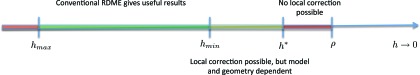
Schematic representation of the RDME's behavior as a function of the voxel size h. For h < h*, no local correction to the conventional mesoscopic reaction rates exists that will make the RDME consistent with the Smoluchowski model for the simple problem of diffusion to a target. Figure adapted from Ref. 90.

Two main approaches have been proposed to improve on the robustness of simulation with the RDME when small length scales need to be considered. The first relies on modification of the bimolecular association reaction rate k_a, as suggested by Isaacson and Isaacson.⁸⁹ For a given k_a and a Cartesian discretization, Erban and Chapman⁸⁶ derived a new rate expression by requiring that the spatially independent steady-state distribution for a model problem solved with the RDME be invariant under changes to the voxel size. Fange et al.⁸⁷ derived mesh dependent propensities in both 2D and 3D based on the ansatz that the equilibration time for a reversible bimolecular reaction should be the same in the SDLR model and the RDME. Furthermore, they allow for reactions between molecules in neighboring voxels. In this way, they obtain good agreement in numerical experiments between the two models, for mesh resolutions close to the reaction radius ρ. A third set of corrected rate functions was obtained by Hellander et al.⁹⁰ in both 2D and 3D. A problematic aspect of relying on mesh-dependent rate functions is that different approaches lead to different expressions, and they are dependent on the nature of the voxels, the geometry, and the test problem. Another approach to the problem was recently taken by Isaacson,⁹¹ where he constructs a new and convergent form of the RDME based on a discretization of a particle tracking model.⁹² Here, the mesoscopic model is formulated in such a way as to converge to a specific microscopic, continuum model per construction.

The other main approach that has been proposed to make simulations more robust is the use of mesoscopic-microscopic hybrid methods, that switch to the microscopic model whenever microscale resolution is required. Hellander et al.⁹³ use an RDME (mesoscopic) model in combination with a Smoluchowski GFRD (microscopic) model. The microscopic model is used only in the regions of the domain that require a high spatial resolution, where the RDME is not well-defined (such as for binding to a curved membrane), or for those reactions that are strongly diffusion limited. With only a small fraction of the molecules treated microscopically, the hybrid method is capable of accurately resolving the features of the model in Ref. 60. Flegg et al.⁹⁴ studied pure diffusion of particles and focused on the accurate treatment of the transition between the mesoscopic and microscopic methods at an interface in 1D.

In contrast to the approach where the RDME is modified in different ways to support microscopically small voxels, hybrid methods have the potential to greatly speed up simulation of models with scale separation in species molecular populations if microscopic resolution is needed only for parts of the model, or in parts of the computational domain. For the majority of the model, relatively large voxels can be used. However, several issues must be resolved before a mesoscopic-microscopic hybrid method can become a general purpose tool. For example, in Ref. 93 a static partitioning is chosen a priori, which requires information on the degree of diffusion control for a reaction. Criteria to partition a system automatically and adaptively are needed.

ACCOMPLISHMENTS AND CHALLENGES

The area of discrete stochastic simulation of chemically reacting systems has seen many advances in algorithms and theory. During the past decade, fast exact and approximate algorithms have been developed for well-mixed systems, multiscale issues have been addressed, and efficient and robust algorithms have been developed for characterizing rare events and estimating parameters. Spatial stochastic simulation is rapidly becoming better understood, and algorithms and software for spatial stochastic simulation on unstructured meshes have begun to appear. There is a great deal left to be done to accommodate models of all of the mechanisms that occur, for example, in cell biology. At the same time, we have come a long way and have developed an extensive collection of algorithms and theory.

One of the major challenges we see at this point is to make these advances available to practitioners in a form that will allow both flexibility and ease of use. We envision an integrated software environment that makes it easy to build a model, scale it up to increasing complexity including spatial simulation, explore the parameter space, and seamlessly deploy the appropriate computing resources as needed. To this end, we have recently begun to develop a new software platform, StochSS (Stochastic Simulation Service, www.stochss.org). It will incorporate, in addition to ODE and PDE solvers, well mixed stochastic simulations via the algorithms of StochKit2,⁹⁵ and spatial stochastic simulations via the algorithms of URDME.⁷² StochSS will also enable the use of a wide range of distributed cloud and cluster computing resources to make the generation of large ensembles of realizations and large parameter sweeps possible, greatly facilitating a careful statistical analysis for even the most expensive simulations.

References

- Wilhelmy L., Ann. Phys. Chem. 81, 413 (1850); [Google Scholar]; Wilhelmy L., Ann. Phys. Chem. 81, 499 (1850). [Google Scholar]
- Delbrück M., J. Chem. Phys. 8, 120 (1940). 10.1063/1.1750549 [DOI] [Google Scholar]
- McQuarrie D., J. Appl. Probab. 4, 413 (1967). 10.2307/3212214 [DOI] [Google Scholar]
- McAdams H. and Arkin A., Proc. Natl. Acad. Sci. U.S.A. 94, 814 (1997). 10.1073/pnas.94.3.814 [DOI] [PMC free article] [PubMed] [Google Scholar]
- Arkin A., Ross J., and McAdams H., Genetics 149, 1633 (1998). [DOI] [PMC free article] [PubMed] [Google Scholar]
- Elowitz M., Levine A., Siggia E., and Swain P., Science 297, 1183 (2002). 10.1126/science.1070919 [DOI] [PubMed] [Google Scholar]
- Weinberger L., Burnett J., Toettcher J., Arkin A., and Schaffer D., Cell 122, 169 (2005). 10.1016/j.cell.2005.06.006 [DOI] [PubMed] [Google Scholar]
- If the observer knows the initial state x0 only as a random variable with some PDF Q0(x0), then the CME straightforwardly transforms, without change, to an equation for $\sum\nolimits_{{\bf x}_0 } {P({\bf x},t|{\bf x}_0,t_0)Q_0 ({\bf x}_0)d{\bf x}_0 } $∑x0P(x,t|x0,t0)Q0(x0)dx0. But that function is not an “unconditioned” PDF P(x, t), because it is obviously conditioned on the initial distribution Q0. The essential role of an observer in the CME is also illustrated by the fact that in many cases, P(x, t|x0, t0) becomes independent of t as t → ∞ while X(t) does not; in that case, the only thing that eventually stops changing with time is best prediction of X that can be made by an observer who last observed X at time t0.
- Gillespie D., J. Comput. Phys. 22, 403 (1976). 10.1016/0021-9991(76)90041-3 [DOI] [Google Scholar]
- Gillespie D., J. Phys. Chem. 81, 2340 (1977). 10.1021/j100540a008 [DOI] [Google Scholar]
- The derivation of Eq. that was given in Ref. can be briefly summarized as follows: $\pi \sigma _{12}^2 \cdot \bar v_{12} dt$πσ122·v¯12dt is the average “collision volume” that a randomly chosen S2 molecule sweeps out relative to the center of a randomly chosen S1 molecule in time dt. Dividing that collision volume by the system volume Ω gives, because the system is dilute and well-mixed, the probability that the center of the S1 molecule lies inside the collision volume, and hence the probability that the two molecules will collide in the next dt. That collision probability multiplied by qj gives the probability that the two molecules will react in the next dt. And finally, that single-pair reaction probability summed over all x1x2 distinct reactant pairs gives the probability defined in Eq. . If the two reactant molecules are of the same species, say S1, then the number of distinct reactant pairs will instead be x1(x1 − 1)/2. Determining the collision-conditioned reaction probability qj, which will always be some number between 0 and 1, requires additional physical reasoning. The best known example is for the model in which an Rj reaction will occur between the two colliding molecules if and only if their “collisional kinetic energy,” suitably defined, exceeds some threshold value Eth. In that case it can be shown [see for instance Gillespie D., Physica A 188, 404 (1992) ] that qj = exp ( − Eth/kBT), which is the famous Arrhenius factor. 10.1016/0378-4371(92)90283-V [DOI] [Google Scholar]
- Gillespie D., J. Chem. Phys. 131, 164109 (2009). 10.1063/1.3253798 [DOI] [PMC free article] [PubMed] [Google Scholar]; As discussed in Sec. VI of this reference, the analysis leading to the result can be regarded as a refined, corrected, and stochastically extended version of the analysis of Collins F. and Kimball G., J. Colloid Sci. 4, 425 (1949). 10.1016/0095-8522(49)90023-9 [DOI] [Google Scholar]; A derivation of Eq. that is further improved over the one given in the 2009 paper can be found in Secs. 3.7 and 4.8 of Gillespie D. and Seitaridou E., Simple Brownian Diffusion (Oxford University Press, 2012). [Google Scholar]
- Smoluchowski M., Z. Phys. Chem. 92, 129 (1917). [Google Scholar]
- Nakanishi T., J. Phys. Soc. Jpn. 32, 1313 (1972); 10.1143/JPSJ.32.1313 [DOI] [Google Scholar]; Nakanishi T., J. Phys. Soc. Jpn. 40, 1232 (1976). 10.1143/JPSJ.40.1232 [DOI] [Google Scholar]
- Šolc M. and Horsák I., Collect. Czech. Chem. Commun. 37, 2994 (1972); 10.1135/cccc19722994 [DOI] [Google Scholar]; Šolc M. and Horsák I., Collect. Czech. Chem. Commun. 38, 2200 (1973); 10.1135/cccc19732200 [DOI] [Google Scholar]; Šolc M. and Horsák I., Collect. Czech. Chem. Commun. 40, 321 (1975). 10.1135/cccc19750321 [DOI] [Google Scholar]
- Bunker D., Garrett B., Kleindienst T., and G.LongIII, Combust. Flame 23, 373 (1974). 10.1016/0010-2180(74)90120-5 [DOI] [Google Scholar]
- The inversion Monte Carlo method exploits the theorem that, if FY is the cumulative distribution function (CDF) of the random variable Y, then FY(Y) will be the unit-interval uniform random variable U. Thus, if u is a random sample of U, then solving (inverting) FY(y) = u will yield a random sample y of Y. Writing Eq. as the product of $a_0 ({\bf x}){\mathop{\rm e}\nolimits} ^{ - a_0 ({\bf x})\tau } $a0(x)e−a0(x)τ and aj(x)/a0(x) reveals that τ and j are statistically independent random variables with those respective PDFs. Integrating (summing) those PDFs over their respective arguments gives their CDFs, and Eqs. then follow from the inversion method. The generic forms of Eqs. , being such straightforward consequences of applying the inversion Monte Carlo method to the aforementioned PDFs of τ and j, were known long before Gillespie's 1976 paper; e.g., see page 36 of J. Hammersley and D. Handscomb, Monte Carlo Methods (Methuen, 1964). The main contributions of Gillespie's 1976 paper were: (i) proving from simple kinetic theory that bimolecular reactions in a dilute gas, like unimolecular reactions, are describable by propensity functions as defined in ; and (ii) proving that propensity functions as defined in imply that the “time to next reaction” and the “index of next reaction” are random variables distributed according to the joint PDF .
- Gibson M. and Bruck J., J. Phys. Chem. 104, 1876 (2000). 10.1021/jp993732q [DOI] [Google Scholar]
- Gillespie D., Annu. Rev. Phys. Chem. 58, 35 (2007). 10.1146/annurev.physchem.58.032806.104637 [DOI] [PubMed] [Google Scholar]
- Cao Y., Li H., and Petzold L., J. Chem. Phys. 121, 4059 (2004). 10.1063/1.1778376 [DOI] [PubMed] [Google Scholar]
- McCollum J., Peterson G., Cox C., Simpson M., and Samatova N., Comput. Biol. Chem. 30, 39 (2006). 10.1016/j.compbiolchem.2005.10.007 [DOI] [PubMed] [Google Scholar]
- Anderson D., J. Chem. Phys. 127, 214107 (2007). 10.1063/1.2799998 [DOI] [PubMed] [Google Scholar]
- Kurtz T., Ann. Probab. 8, 682 (1980); 10.1214/aop/1176994660 [DOI] [Google Scholar]; Ethier S. and Kurtz T., Markov Processes: Characterization and Convergence (Wiley, 1986). [Google Scholar]
- Anderson D. and Kurtz T., “Continuous time Markov chain models for chemical reaction networks,” in Design and Analysis of Biomolecular Circuits: Engineering Approaches to Systems and Synthetic Biology, edited by Koeppl H.et al. (Springer, 2011). [Google Scholar]
- Slepoy A., Thompson A., and Plimpton S., J. Chem. Phys. 128, 205101 (2008). 10.1063/1.2919546 [DOI] [PubMed] [Google Scholar]
- Mauch S. and Stalzer M., IEEE/ACM Trans. Comput. Biol. Bioinf. 8, 27 (2011). 10.1109/TCBB.2009.47 [DOI] [PubMed] [Google Scholar]
- Gillespie D., J. Chem. Phys. 115, 1716 (2001). 10.1063/1.1378322 [DOI] [Google Scholar]
- An early conjecture was that the negativity problem in tau-leaping was caused by the unbounded Poisson random variables in the tau-leaping formula occasionally allowing too many reaction firings in a single leap. That conjecture led to proposals to replace the Poisson random variables in Eq. with binomial random variables, which are bounded. But it was subsequently determined that the principal causes of the negativity problem lay elsewhere. First was the flawed implementation of the leap condition that was used in Ref. : the small-valued propensity functions that it failed to protect often have a reactant with a small molecular population which can easily be driven negative. Second, since the firing numbers of the individual reactions in the tau-leaping formula are generated independently of each other, two or more reaction channels that decrease the population of a common species could inadvertently collude to overdraw that species. Neither of these two problems is fixed by the ad hoc substitution of binomial random variables for the Poisson random variables in Eq. . But both problems are effectively dealt with in the heavily revised tau-leaping procedure described in Ref. , which uses the theoretically appropriate Poisson random variables.
- Cao Y., Gillespie D., and Petzold L., J. Chem. Phys. 124, 044109 (2006). 10.1063/1.2159468 [DOI] [PubMed] [Google Scholar]
- Gillespie D., “Simulation methods in systems biology,” in Formal Methods for Computational Systems Biology, edited by Bernardo M., Degano P., and Zavattaro G. (Springer, 2008), pp. 125–167, Sec. 3 gives a tutorial on tau-leaping, Secs. 4 and 5 give a tutorial on the ssSSA. [Google Scholar]
- Rathinam M., Petzold L., Cao Y., and Gillespie D., J. Chem. Phys. 119, 12784 (2003); 10.1063/1.1627296 [DOI] [Google Scholar]; Rathinam M., Petzold L., Cao Y., and Gillespie D., J. Chem. Phys. 121, 12169 (2004); 10.1063/1.1823412 [DOI] [PubMed] [Google Scholar]; Rathinam M., Petzold L., Cao Y., and Gillespie D., Multiscale Model. Simul. 4, 867 (2005). 10.1137/040603206 [DOI] [Google Scholar]
- Auger A., Chatelain P., and Koumoutsakos P., J. Chem. Phys. 125, 084103 (2006). 10.1063/1.2218339 [DOI] [PubMed] [Google Scholar]
- Anderson D., J. Chem. Phys. 128, 054103 (2008). 10.1063/1.2819665 [DOI] [PubMed] [Google Scholar]
- The view we have taken here of dt as an independent real variable on the interval [0, ɛ), where ɛ is an arbitrarily small positive number, means that $\sqrt {dt} $dt in Eq. is perfectly well defined. For an explanation of the connection between the factor ${\cal N}_j (0,1)\sqrt {dt}$Nj(0,1)dt in Eq. and “Gaussian white noise,” see Gillespie D., Am. J. Phys. 64, 225 (1996); 10.1119/1.18210 [DOI] [Google Scholar]; Gillespie D., Am. J. Phys. 64, 1246 (1996). 10.1119/1.18387 [DOI] [Google Scholar]
- Gillespie D., J. Chem. Phys. 113, 297 (2000). The CLE can be shown to be mathematically equivalent to the Fokker-Planck equation that is obtained by first making a formal Taylor series expansion of the right side of the CME , which yields the so-called Kramers-Moyal equation, and then truncating that expansion after the second derivative term. However, that way of “obtaining” the CLE, which was known well before this 2000 paper, does not qualify as a derivation, because it does not make clear under what conditions the truncation will be accurate. In contrast, the derivation of the CLE given here provides a clear and testable criterion for the accuracy of its approximations, namely, the extent to which both leap conditions are satisfied. But see also the proviso in Ref. . 10.1063/1.481811 [DOI] [Google Scholar]
- The approximation ${\cal P}(m) \approx {\cal N}(m,m)$P(m)≈N(m,m) that was made in deriving the CLE from the tau-leaping formula , while accurate for likely values of those two random variables, is very inaccurate in the tails of their probability densities, even when m ≫ 1. Although both tails are “very near 0,” they differ by many orders of magnitude. Since rare events arise from the “unlikely” firing numbers under those tails, it follows that the CLE will not accurately describe the atypical behavior of a chemical system, even if both leap conditions are well satisfied.
- Gillespie D., J. Phys. Chem. B 113, 1640 (2009). 10.1021/jp806431b [DOI] [PMC free article] [PubMed] [Google Scholar]
- The foregoing chain of reasoning can be summarized from the perspective of computational mathematics as follows: The definition of the propensity function implies, for any time step τ that is small enough to satisfy the first leap condition , the tau-leaping formula . If the second leap condition is also satisfied, the tau-leaping formula becomes Eq. , which is the forward Euler formula for a stochastic differential equation. And that formula becomes in the thermodynamic limit, where its diffusion term will be negligibly small compared to its drift term, the forward Euler formula for an ordinary differential equation.
- A common misconception is that, while the molecular population X is obviously a discrete variable, the molecular concentration Z ≡ X/Ω is a “continuous” variable. The error in that view becomes apparent when one realizes that simply by adopting a unit of length that gives Ω the value 1, Z becomes numerically equal to X. But even if that is not done, a sudden change in X, say from 10 to 9, will always result a discontinuous 10% decrease in Z. The molecular concentration Z is no less discrete, and no more continuous, than the molecular population X.
- Kurtz T., Stochastic Proc. Appl. 6, 223 (1978). 10.1016/0304-4149(78)90020-0 [DOI] [Google Scholar]
- van Kampen N., Adv. Chem. Phys. 34, 245 (1976); 10.1002/9780470142530.ch5 [DOI] [Google Scholar]; Stochastic Processes in Physics and Chemistry (North-Holland, 1992). [Google Scholar]
- Wallace E., Gillespie D., Sanft K., and Petzold L., IET Syst. Biol. 6, 102 (2012). 10.1049/iet-syb.2011.0038 [DOI] [PubMed] [Google Scholar]
- Grima R., Thomas P., and Straube A., J. Chem. Phys. 135, 084103 (2011). 10.1063/1.3625958 [DOI] [PubMed] [Google Scholar]
- The last step in Eq. can be heuristically understood as follows: The integral $\int_{t_0 }^t {{\cal P}_j \left( {a_j \!\left( {{\bf X}(t^\prime)} \right) dt^\prime } \right)}$∫t0tPjajX(t′)dt′ is essentially a sum of independent Poisson random variables, each indexed by t′ and having mean aj(X(t′))dt′. An established result in random variable theory is that the sum of K independent Poisson random variables with means m1, …, mK is a Poisson random variable with mean $\sum\nolimits_{k = 1}^K {m_k } $∑k=1Kmk. Therefore, the integral $\int_{t_0 }^t {{\cal P}_j ( {a_j ( {{\bf X}(t^\prime)} )\,dt^\prime } )}$∫t0tPj(aj(X(t′))dt′) in Eq. is a Poisson random variable with mean $\int_{t_0 }^t {a_j ( {{\bf X}(t^\prime)} )\,dt^\prime } $∫t0taj(X(t′))dt′. For an explanation of how that Poisson random variable can be viewed as a “unit-rate Poisson process” Yj that is “scaled” by $\int_{t_0 }^t {a_j \!\left( {{\bf X}(t^\prime)} \right)dt^\prime } $∫t0tajX(t′)dt′, see Refs. and . Note that all the integrals here can be written as finite algebraic sums, since X(t′) stays constant between successive reactions.
- Cao Y., Gillespie D., and Petzold L., J. Chem. Phys. 122, 014116 (2005); 10.1063/1.1824902 [DOI] [PubMed] [Google Scholar]; Cao Y., Gillespie D., and Petzold L., J. Chem. Phys. 123, 144917 (2005). 10.1063/1.2052596 [DOI] [PubMed] [Google Scholar]; A more concise tutorial presentation of the ssSSA, featuring illustrative applications to reactions and the classical enzyme-substrate reactions E + S ⇌ ES → E + P, is given in Ref. . A more thorough examination of the relation between the ssSSA's treatment of the enzyme-substrate system and the classical Michaelis-Menten approximation is given in Sanft K., Gillespie D., and Petzold L., IET Syst. Biol. 5, 58 (2011). 10.1049/iet-syb.2009.0057 [DOI] [PubMed] [Google Scholar]
- Under the condition c2 ≫ c3, R1 will be a “fast” reaction regardless of the size of c1. That is because the conversion of an S1 molecule into an S3 molecule necessarily takes exactly one more R1 reaction than R2 reaction. Thus, in most time intervals there will be at least as many R1 firings as R2 firings; hence, if R2 is fast, then R1 must be also. This illustrates the important fact that fast and slow reaction channels cannot always be identified solely on the basis of the magnitudes of their rate constants.
- Cao Y., Gillespie D., and Petzold L., J. Comput. Phys. 206, 395 (2005). 10.1016/j.jcp.2004.12.014 [DOI] [Google Scholar]
- Ferm L., Lotstedt P., and Hellander A., J. Sci. Comput. 34, 127 (2008). 10.1007/s10915-007-9179-z [DOI] [Google Scholar]
- Singh A. and Hespanha J., IEEE Trans. Autom. Control. 56, 414 (2011). 10.1109/TAC.2010.2088631 [DOI] [Google Scholar]
- E W., Liu D., and Vanden-Eijnden E., J. Chem. Phys. 123, 194107 (2005); 10.1063/1.2109987 [DOI] [PubMed] [Google Scholar]; Gillespie D., Petzold L., and Cao Y., J. Chem. Phys. 126, 137101 (2007). 10.1063/1.2567036 [DOI] [PubMed] [Google Scholar]
- Sanft K., Ph.D. thesis, University of California, Santa Barbara, 2012. [Google Scholar]
- Kuwahara H. and Mura I., J. Chem. Phys. 129, 165101 (2008). 10.1063/1.2987701 [DOI] [PubMed] [Google Scholar]
- Gillespie D., Roh M., and Petzold L., J. Chem. Phys. 130, 174103 (2009). 10.1063/1.3116791 [DOI] [PMC free article] [PubMed] [Google Scholar]
- Roh M., Gillespie D., and Petzold L., J. Chem. Phys. 133, 174106 (2010). 10.1063/1.3493460 [DOI] [PMC free article] [PubMed] [Google Scholar]
- B.Daigle, Jr., Roh M., Gillespie D., and Petzold L., J. Chem. Phys. 134, 044110 (2011). 10.1063/1.3522769 [DOI] [PMC free article] [PubMed] [Google Scholar]
- Roh M., B.Daigle, Jr., Gillespie D., and Petzold L., J. Chem. Phys. 135, 234108 (2011). 10.1063/1.3668100 [DOI] [PMC free article] [PubMed] [Google Scholar]
- Rubinstein R. and Kroese D., The Cross-Entropy Method (Springer, 2004). [Google Scholar]
- Rathinam M., Sheppard P., and Khammash M., J. Chem. Phys. 132, 034103 (2010). 10.1063/1.3280166 [DOI] [PMC free article] [PubMed] [Google Scholar]
- Anderson D., SIAM J. Numer. Anal. 50, 2237 (2012). 10.1137/110849079 [DOI] [Google Scholar]
- Takahashi K., Tănase-Nicola S., and ten Wolde P., Proc. Natl. Acad. Sci. U.S.A. 107, 2473 (2010). 10.1073/pnas.0906885107 [DOI] [PMC free article] [PubMed] [Google Scholar]
- Doubrovinski K. and Howard M., Proc. Natl. Acad. Sci. U.S.A. 102, 9808 (2005). 10.1073/pnas.0500529102 [DOI] [PMC free article] [PubMed] [Google Scholar]
- Elf J. and Ehrenberg M., Syst. Biol. 1, 230 (2004). 10.1049/sb:20045021 [DOI] [PubMed] [Google Scholar]
- Metzler R., Phys. Rev. Lett. 87, 068103 (2001). 10.1103/PhysRevLett.87.068103 [DOI] [PubMed] [Google Scholar]
- Sturrock M., Hellander A., Matzavinos M., and Chaplain M., J. R. Soc. Interface 10, 20120988 (2013). 10.1098/rsif.2012.0988 [DOI] [PMC free article] [PubMed] [Google Scholar]
- Fange D. and Elf J., PLoS Comput. Biol. 2(6), e80 (2006). 10.1371/journal.pcbi.0020080 [DOI] [PMC free article] [PubMed] [Google Scholar]
- Gardiner C., McNeil K., Walls D., and Matheson I., J. Stat. Phys. 14, 307 (1976). 10.1007/BF01030197 [DOI] [Google Scholar]
- See, for example, Gillespie D. and Seitaridou E., Simple Brownian Diffusion (Oxford University Press, 2012), Chap. 5. That chapter's revised Sec. 5.6 (which can be downloaded from the book's webpage on the publisher's website) shows that below a certain value of h, no propensity function can give a physically accurate modeling of diffusive transfers of molecules between voxels. [Google Scholar]
- Equation also follows by applying the “centered finite difference method” in numerical analysis to the diffusion Eq. .
- Kurtz T., J. Appl. Probab. 7, 49 (1970). 10.2307/3212147 [DOI] [Google Scholar]
- Isaacson S. and Peskin C., SIAM J. Sci. Comput. 28, 47 (2006). 10.1137/040605060 [DOI] [Google Scholar]
- Isaacson S., McQueen D., and Peskin C., Proc. Nat. Acad. Sci. U.S.A. 108, 3815 (2011). 10.1073/pnas.1018821108 [DOI] [PMC free article] [PubMed] [Google Scholar]
- Engblom S., Ferm L., Hellander A., and Lötstedt P., SIAM J. Sci. Comput. 31, 1774 (2009). 10.1137/080721388 [DOI] [PMC free article] [PubMed] [Google Scholar]
- Drawert B., Engblom S., and Hellander A., BMC Syst. Biol. 6, 76 (2012). 10.1186/1752-0509-6-76 [DOI] [PMC free article] [PubMed] [Google Scholar]
- Kang H.-W., Zheng L., and Othmer H., J. Math. Biol. 65, 1017 (2012). 10.1007/s00285-011-0469-6 [DOI] [PMC free article] [PubMed] [Google Scholar]
- Rossinelli D., Bayati B., and Koumoutsakos P., Chem. Phys. Lett. 451, 136 (2008). 10.1016/j.cplett.2007.11.055 [DOI] [Google Scholar]
- Iyengar K., Harris L., and Clancy P., J. Chem. Phys. 132, 094101 (2010). 10.1063/1.3310808 [DOI] [PubMed] [Google Scholar]
- Marquez-Lago T. and Burrage K., J. Chem. Phys. 127, 104101 (2007). 10.1063/1.2771548 [DOI] [PubMed] [Google Scholar]
- Lampoudi S., Gillespie D., and Petzold L., J. Chem. Phys. 130, 094104 (2009). 10.1063/1.3074302 [DOI] [PMC free article] [PubMed] [Google Scholar]
- Koh W. and Blackwell K., J. Chem. Phys. 134, 154103 (2011). 10.1063/1.3572335 [DOI] [PMC free article] [PubMed] [Google Scholar]
- Drawert B., Lawson M., Petzold L., and Khammash M., J. Chem. Phys. 132, 074101 (2010). 10.1063/1.3310809 [DOI] [PMC free article] [PubMed] [Google Scholar]
- Ferm L., Hellander A., and Lötstedt P., J. Comput. Phys. 229, 343 (2010). 10.1016/j.jcp.2009.09.030 [DOI] [Google Scholar]
- Gillespie D., Lampoudi S., and Petzold L., J. Chem. Phys. 126, 034302 (2007). 10.1063/1.2424461 [DOI] [PubMed] [Google Scholar]
- Lampoudi S., Gillespie D., and Petzold L., J. Comput. Phys. 228, 3656 (2009). 10.1016/j.jcp.2009.02.002 [DOI] [PMC free article] [PubMed] [Google Scholar]
- Grima R., J. Chem. Phys. 132, 185102 (2010). 10.1063/1.3427244 [DOI] [Google Scholar]
- Zon J., van Zon S., and Rein ten Wolde P., Phys. Rev. Lett. 94, 128103 (2005). 10.1103/PhysRevLett.94.128103 [DOI] [PubMed] [Google Scholar]
- Erban R. and Chapman J., Phys. Biol. 6, 046001 (2009). 10.1088/1478-3975/6/4/046001 [DOI] [PubMed] [Google Scholar]
- Fange D., Berg O. G., Sjöberg P., and Elf J., Proc. Natl. Acad. Sci. U.S.A. 107, 19820 (2010). 10.1073/pnas.1006565107 [DOI] [PMC free article] [PubMed] [Google Scholar]
- Isaacson S., SIAM J. Appl. Math. 70, 77 (2009). 10.1137/070705039 [DOI] [Google Scholar]
- Isaacson S. and Isaacson D., Phys. Rev. E 80, 066106 (2009). 10.1103/PhysRevE.80.066106 [DOI] [PMC free article] [PubMed] [Google Scholar]
- Hellander S., Hellander A., and Petzold L., Phys. Rev. E 85, 042901 (2012). 10.1103/PhysRevE.85.042901 [DOI] [PubMed] [Google Scholar]
- Isaacson S., “A convergent reaction-diffusion master equation,” preprint arXiv:1211.6772v1 (2012). [DOI] [PubMed]
- Doi M., J. Phys. A: Math. Gen. 9, 1465 (1976); 10.1088/0305-4470/9/9/008 [DOI] [Google Scholar]; Doi M., J. Phys. A: Math. Gen. 9, 1479 (1976). 10.1088/0305-4470/9/9/009 [DOI] [Google Scholar]
- Hellander A., Hellander S., and Lötstedt P., Multiscale Model. Simul. 10, 585 (2012). 10.1137/110832148 [DOI] [PMC free article] [PubMed] [Google Scholar]
- Flegg M., Chapman S., and Erban R., J Roy. Soc. Interface 9, 859 (2012). 10.1098/rsif.2011.0574 [DOI] [PMC free article] [PubMed] [Google Scholar]
- Sanft K., Wu S., Roh M., Fu J., Lim R., and Petzold L., Bioinformatics 27, 2457 (2011). 10.1093/bioinformatics/btr401 [DOI] [PMC free article] [PubMed] [Google Scholar]