Leveraging Social Networks for Toxicovigilance

Abstract

The landscape of drug abuse is shifting. Traditional means of characterizing these changes, such as national surveys or voluntary reporting by frontline clinicians, can miss changes in usage the emergence of novel drugs. Delays in detecting novel drug usage patterns make it difficult to evaluate public policy aimed at altering drug abuse. Increasingly, newer methods to inform frontline providers to recognize symptoms associated with novel drugs or methods of administration are needed. The growth of social networks may address this need. The objective of this manuscript is to introduce tools for using data from social networks to characterize drug abuse. We outline a structured approach to analyze social media in order to capture emerging trends in drug abuse by applying powerful methods from artificial intelligence, computational linguistics, graph theory, and agent-based modeling. First, we describe how to obtain data from social networks such as Twitter using publicly available automated programmatic interfaces. Then, we discuss how to use artificial intelligence techniques to extract content useful for purposes of toxicovigilance. This filtered content can be employed to generate real-time maps of drug usage across geographical regions. Beyond describing the real-time epidemiology of drug abuse, techniques from computational linguistics can uncover ways that drug discussions differ from other online conversations. Next, graph theory can elucidate the structure of networks discussing drug abuse, helping us learn what online interactions promote drug abuse and whether these interactions differ among drugs. Finally, agent-based modeling relates online interactions to psychological archetypes, providing a link between epidemiology and behavior. An analysis of social media discussions about drug abuse patterns with computational linguistics, graph theory, and agent-based modeling permits the real-time monitoring and characterization of trends of drugs of abuse. These tools provide a powerful complement to existing methods of toxicovigilance.

Introduction

Existing approaches to address drug abuse patterns across a given region include federally sponsored surveys, reports from National Poisoning Data System, the Food and Drug Administration, and reports from hospital networks such as the Drug Abuse Warning Network. Surveys such as the National Survey on Drug Use and Health, while rigorously documenting usage by frequency, location, and demographics, have limitations. They are infrequently updated, and do not collect information on newer drugs of abuse [1]. Poison control centers and hospital networks rely on either phone calls or hospitalizations, which the users of newer drugs may not generate.

Recent reports point to an emergence of new drugs of abuse such as “bath salts”, synthetic cannabinoids, and Salvia divinorum. Since existing methods of drug surveillance may not capture the demographics or geographic distribution of usage associated with these newer substances, frontline providers are therefore less familiar with local terminology and drug prevalence, and less acquainted with the signs and symptoms associated with these drugs. Furthermore, public health officials at state and local levels could also use this information to better allocate resources for substance abuse prevention, recognition, and intervention [2].

Many of the techniques we will describe will refer to applications for toxicovigilance. For the purposes of this paper, we will define “toxicovigilance” as the active process of identification, investigation, and evaluation of the various toxic risks in the community with a view to taking measures to reduce or eliminate these risks [3]. The toxic risks discussed in this paper will almost exclusively refer to drugs of abuse as opposed to industrial or occupational toxins and apply to those who use social media, a population that may be a biased sample of a region.

Social network data is especially suited to provide insights into patterns of use for novel drugs of abuse. Platforms such as Twitter, Facebook, and YouTube facilitate the exchange of short messages, via desktop, laptop, tablet, or smart phone between members of interrelated groups. In other realms of medicine, such as infectious disease and public health, social network messages have been analyzed for syndromic surveillance and disease sentiment analysis [4, 5]. Thus, there is precedent for the incorporation of social network data for epidemiological interpretation.

For medical toxicologists, social networks provide an appropriate means of assessing patterns of drugs of abuse; the effects of many drugs facilitate expressive communication and peer impressions often provide the lens by which these drug effects are sought and perceived. There is already evidence that social networks have been employed by drug abusers for the purpose of discussing and obtaining drugs [6, 7]. Researchers have begun to study the content of messages shared on these networks, to characterize the introduction of new drugs [8].

A systematic approach to analyzing content from social networks has the potential to overcome several deficiencies of current methods of characterizing drug usage patterns, while preserving some of the existing tools’ best attributes. Like many surveys, the data obtained from these social messages is tagged by location, but has the advantage of real-time updates, facilitating a more dynamic epidemiology. Like reports from poison control centers and inpatient networks, new drugs of abuse can be uncovered via social networks, but without the distortion that comes with contact (by a call or hospitalization) with the healthcare system. Pros and cons of content analysis using traditional tools versus social networks are outlined in Table 1.

Table 1.

Advantages and disadvantages of traditional tools of toxicovigilance, and drug surveillance via social networks

	Traditional tools of toxicovigilance	Social network tools
Pros	• Validated methodology	• Rapidly updating
	• Established infrastructure	• Deep source of data
	• Large amount of baseline data	• Amenable to online analysis
	• Usually well-funded by federal and private organizations	• No funding necessary to generate data
	• Intended for clinical or epidemiological use	• No time lag
Cons	• Infrequently updated	• Untested
	• Poor at discovering new drugs	• May be easier to manipulate
	• Data are hard to access	• No precedent in the medical literature
	• Data ownership may limit analysis	• Results might not generalize to those not using social media
	• Time lag for new epidemics or abuse trends
	• Reporting bias

Compared to current methods of drug abuse surveillance, perhaps the greatest limitation to analysis of social networks is the relative lack of socioeconomic and demographic information available from users and behaviors surrounding usage. But even this challenge can be addressed with the tools of graph theory and agent-based modeling to shed light on the characteristics of discussants and inferences of attitudes and behaviors from online discussions.

The objective of this manuscript is to discuss novel and productive techniques for using social media to analyze drug abuse trends for toxicovigilance, to highlight strengths and weaknesses of each technique, and to identify how these techniques may complement traditional methods of toxicovigilance.

Social Networks as a Data Source for Toxicovigilance

Social networks can provide medical toxicologists with real-time information on emergence and usage of drugs; the data from these networks must be appropriately analyzed to construct models that predict changes in the patterns of drug abuse, and detect the emergence of new drugs. Using social media as a data source means making inferences and predictions based on these models and should agree with official data sources when available.

The following subsections sketch ways for medical toxicologists to extract reliable information on drug abuse from social media and how to use them to build predictive models. Because there are many social media sites, none of the methods described here are specific to only one social media site. They do, however, assume that the site provides and automated programmatic interface (API). An API allows software components to interface with each other and social networks such as Twitter, Facebook, Google+, LinkedIn, Tumblr, and YouTube, provide APIs. Typically, those APIs have different levels of access for the general public and for software developers. APIs only have access to information that is in the public domain. For example, if a user does not make his Facebook page publicly discoverable, then an API will never return data about this user. This restriction could contribute to a sampling bias.

Limitations are to be expected when listening in on a national conversation. Dealing with slang and regional dialects is a major challenge. Strategies, such as creating annotated linguistic corpora related to drug use, are only beginning to emerge. Furthermore, even though social network usage is increasingly common, it still gives biased sample of the general American population. Determining how the cross-section of social network users relates to the general American population—let alone the subset of those who candidly discuss drug usage—is not yet established.

Conventions Used

The methods this paper discusses require the textual data to be preprocessed. In particular, the reader should assume that all punctuation marks and anything that is not a letter in the unaccented Roman alphabet has been removed, the text converted to lower case, and all words stemmed. (Stemming refers to removing all affixes. For example, stemming reduces “rider”, “riding”, “riders”, and “ridden” all to “ride”). Finally, the authors exclude symbols that cannot be encoded in the American Standard Code for Information Interchange. The authors choose to do this because they focus on English, which does not use diacritical marks such as accents and is the predominant language on Twitter. All the methods that this paper discussed also apply to languages that use the Roman alphabet with accents and languages such as Greek, Arabic, and Hebrew that use different alphabets. In that case, all data would be encoded in unicode and each language would need its own analysis pipeline.

Methods for Analyzing Social Networks

Natural Language Processing

The tools to find meaning and structure in large sets of social network messages belong to the field of natural language processing (NLP). NLP attempts to enable computers to understand human language as humans do. Characteristic areas range from accurate automatic translation between languages to more complex problems such as analyzing the meaning or symbolisms of a piece of text.

NLP can uncover statistical structures in a dataset. If physicians also evaluate that dataset, the machine learning techniques described above can apply statistical structures to predict those physicians’ evaluations. For medical toxicologists, this combination of NLP and machine learning may provide a generalizable approximation to clinical intuition. Throughout this section, these methods will be illustrated through the content of one tweet, hereafter referred to as tweet A: “Heading out tonight to meet friends, do some cocaine. Gotta love cocaine!”

The main limitation of all natural language processing methods is that they are only approximations of human communication and may miss important subtleties that limit the ability of these methods to understand and draw inferences from human communication.

Frequency Analysis

Frequency analysis is a simple screening tool to help characterize a document by identifying its most and least frequent words. For example, if the data resemble standard American English, then its most frequent words will closely match those of standard American English. Deviations from that expected concordance may be informative. For example, the most common word in tweet A is cocaine, which is not the most common word in the American English language. Even accounting for the brevity of tweets, this divergence suggests further investigation.

One can refine basic frequency analysis by omitting various classes of words that are typically uninformative. For example, one can omit words that occur extremely often—stop words, such as “the”, “to”, and “also”. Leaving them out may uncover the most frequent words specific to the data’s topic. Those will be more helpful when training artificial intelligence algorithms to identify the topic to which the data belong. Finding specific features, such as keywords, greatly improves the accuracy of classifiers. The section on machine learning discusses this further. Removing stop words (and grammar) from tweet A would yield the reduced tweet “heading tonight meet friends some cocaine love cocaine.”

A further refinement is to look for the most frequently occurring words that have a minimum length. However, this restriction may be inappropriate for social media such as Twitter that limit the length of each message or that often use abbreviations. For example “jk”, an abbreviation meaning “just kidding” can dramatically change the meaning of a tweet.

Determining the least frequent words in a document may also be useful. Similarly, the absence of certain words might indicate a topic just as specifically as the presence of others. Characteristic omissions may be informative, especially when analyzing conversations that discuss illegal activities.

With any analysis that compares data from social media against a point of reference, that point of reference must be narrowly defined. For example, the dialectal differences among American, British, and Standard Singapore English mean that different lists of stop words should be used for each. Dialectal differences become especially important when considering slang words and abbreviations.

Collocations

Frequency analysis helps to identify keywords. However, because it ignores the statistical relationships between words, frequency analysis alone gives a shallow description of the data. For example, frequency analysis measures how frequent a word is in general, but not how frequently it occurs after another word.

A collocation is a sequence of words that occurs together unusually often. A very useful characteristic of collocations is that substituting one word with another in a collocation sounds very odd, even if those two words are homonyms. For example, “maroon wine” sounds stranger than “red wine” even though “red” and “maroon” are more similar colors than “red” and “white”. Analyzing text for groups of words whose homonyms form collocations provides a way to detect new terms discussing a drug.

Finding collocations requires a large amount of data because determining them requires one to estimate the frequency of occurrence of every possible pair of words in a document. For short messages, such as tweets, these are computed from large databases of at least one million unique tweets. This requirement also applies to lexical diversity and Lempel–Ziv complexity, which are discussed below.

n-Grams

An n-gram is a contiguous sequence of n words. The previous sentence is a nine-gram. Both collocations and the frequency of single words are special cases of n-grams. Collocations are bigrams that occur more frequently than should happen by chance alone. For more discussion on n-grams, see Cavnar and Trenkle [9].

n-Grams may help identify novel synonyms for or symptoms associated with a drug. For example, a word that describes a new method of insufflating cocaine might be used similarly to “snort”. Suppose the new method of insufflation is called “slalom”. Then, the collocation [slalom cocaine] will be expected to appear nearly as often as [snort cocaine].

Lexical Diversity and Lempel–Ziv Complexity

Lexical diversity and Lempel–Ziv complexity are two related measures of how much unique content a message has. Lexical diversity is the ratio of the number of unique words in a document to the total number of words, often defined to keep the range of all their measurements between 0 and 1.

Lempel–Ziv complexity (LZ) is the ratio of the number of unique symbols in a document to the total number of symbols (a symbol is a group of words) [10]. Whereas lexical diversity counts redundant words, LZ counts redundant symbols, compressing n-grams as well as words. For social network toxicovigilance, the authors plan to use a modification of the original LZ method that corrects for errors that occur when dealing with short string of text such as tweets or YouTube comments [11].

Machine Learning for Social Network Toxicovigilance

Machine learning is a field of artificial intelligence that tries to infer relationships in a set of data, viewing data as resulting from the interactions of variables, and trying to discover those variables from the data. Machine learning is employed in social network toxicovigilance in two ways: first, to isolate relevant items from the stream of social media data. Second, machine learning is employed to discover how relationships among those variables change over time. Both uses are incarnations of one fundamental process in machine learning–classifying text [12].

The biggest limitation in applying techniques from machine learning to toxicology is that these techniques work best when supplied with large amounts of training data. In practice, this means that toxicologists need to periodically review the output of machine learning algorithms as part of an ongoing quality assessment. Machine learning algorithms perform poorly on extremely novel data and are only able to learn some of the relationships that link data in a dataset.

Classification is the grouping of objects into similar clusters where each cluster shares common features. For example, the authors plan to filter out social media data useful for toxicovigilance, by categorizing each document as “useful” or “not useful”. Each category is defined by the 50 most frequent words that occur in that category and in no other category. A piece of text belongs to the category to which its words are most common. Partial membership may be allowed for data that fall equally between two categories.

Feature Selection

The choice of features heavily influences how accurate a classifier can be. The right features depend greatly on the specific type of classifier being developed. For example, if the feature of the average length of a word in a document was chosen, instead of the frequency of a word, filters would probably perform very poorly. However, the average word length is a useful feature for characterizing the context-free complexity of a document (this is why average word length is sometimes presented alongside calculations of the Flesch–Kincaid grade level, in documents).

Usually, the right features are determined through iterative testing on multiple curated datasets and statistical techniques, such as singular value decomposition to identify which features are the most informative. For the iterative testing, we prepare many independent datasets. For example, we could sample tweets from Twitter daily and combine those tweets into one large database. From that database, we could retrieve ten random samplings of tweets across all dates. This would provide the data for ten rounds of testing. At each round, human experts and the classifier rate the same data (to determine, for instance, if a tweet or comment denotes recent drug use). We investigate the discrepancy between those two groups of ratings for systematic differences that can be addressed, such as the classifier mistaking a quoted music lyric for actual intention to use drugs.

Statistical techniques such as singular value decomposition (see Fig. 1) are complementary to this process. Singular value decomposition, which is also called latent semantic analysis, finds the most informative combinations of words in a document. Here, “most informative” means recreates the most documents the most accurately with the least number of words [13]. To briefly describe the process, first, a (t)erm (f)requency–(i)nverse (d)ocument (m)atrix is formed. In that matrix, each row is an utterance, for example a tweet or YouTube comment. Each entry in the row indicates the number of times a word appears in the utterance to which that row corresponds (term frequency) and can be scaled by how often that word occurs across all documents (inverse document frequency). Then, the tf–idf matrix is decomposed into the product of three matrices, U, S, and V. The columns of U describe how similar the group of tweets or comments are. The rows of V describe how frequently the same words appear together across the utterances. The values of the diagonal of S, the singular values, show the relative importance of each of the columns of the original matrix in describing all the utterances. Here, “I” has the highest singular value because it occurs in all documents. Words such as “I” are commonly removed because their singular values would dominate any document and so are nonspecific.

Fig. 1.

Singular value decomposition for extracting features from text. Example SVD for three tweets. The upper left entry of Σ is the greatest and so the first row of V and column of U explain the largest amount of text. Notice that because the pronoun “I” occurs in all tweets, it is not a distinguishing feature. However, its prevalence biases the estimation of the singular values. This is the rationale for removing stopwords

However, singular value decomposition and a nonparametric version, latent Dirichlet allocation, only capture the most informative combinations of words without paying attention to the grammar of the document. Ignoring grammatical structure makes the algorithms much faster but at the expense of loosing the ability to differentiate between well-structured thoughts and “word salad” [14]. Ignoring grammar also impairs the ability of “bag of words” classifiers to detect emotions or subtext in a document.

A major problem with training classifiers is overfilling them to the training data. Often, features that allow spectacular performance on test data are different from those that work after deployment. This suggests that choosing the “most informative” features may be applying a misguided criterion. Furthermore, the best features may change over time, especially in social media, which is rife with slang and trending topics.

Naive Bayes Classifier

A naive Bayes classifier categorizes a document into three stages. First, it calculates the chance that, with no further information, a piece of text could belong to each category—the prior probability. For example, if there are ten categories, the prior probability would be 10 % for each category. Then, for each category for which the document has words (features) that identify that category, the probability that the document belongs to that category is augmented. Finally, the document is assigned to the category to which it has the highest probability of belonging. Central to a naives Bayes classifier is the naive Bayes assumption. This assumes that the features the classifiers uses are independent. If the data have only second-order correlations, then approaches such as singular value decomposition or principal components analysis will yield independent features. Singular value decomposition is a decomposition of one matrix into a product of three matrices—the left eigenvectors, eigenvalues, and right eigenvectors of the original matrix. Principal components analysis is a special case of singular value decomposition when the matrix is square and so the left and right eigenvectors are identical. In either case, each eigenvector is linearly independent with respect to all other eigenvectors. The eigenvectors, then, are the first-order approximation to the most independent, and so most informative, features in the data. However, when higher-order correlations such as collocations are prominent, a naive Bayes classifier based on features derived with singular value decomposition or principal components analysis will perform poorly because those methods are only first-order approximations.

Example from Social Network Toxicovigilance

The authors plan to examine tweets and rate the likelihood that they were discussing likely immediate drug usage (such as Tweet A, discussed previously). Then, they will use a naive Bayes classifier to determine which features of those tweets most accurately predicted the authors’ ratings. Applying a classifier to a data set rated by physicians is called training the classifier. Once trained, the classifier can rate new, larger datasets and so act as a proxy for physicians reviewing those data. The data used to train a classifier should be representative of the data the classifier will encounter. Otherwise, the classifier will be unable to generalize and will be a poor surrogate for clinical judgment.

Graph Theory for Social Network Toxicovigilance

Graph theory studies structures called graphs that model pairwise interactions between objects (see Fig. 2). For graphs of social networks, the nodes represent people and the edges interactions between two people. It is easy to apply graph theory to online social networks such as Facebook and Twitter. Typical actions on those networks, such as following a particular user on Twitter, or disrupting a connecting by “unfriending” someone on Facebook, correspond to the creation and destruction of edges. One productive way to describe the evolution of a graph of a social network is to track how the distributions of edges (interactions) and nodes (people) change over time. For a more mathematical reference, see Bondy and Murty [15].

Fig. 2.

Schematic of a social network graph. Lines (edges) extend from one user to another if that first user retweets (RT) that message

Detecting Communities of Drug Users

Individuals who use social networks are more likely to associate with one another if they share common interests. That is, like goes with like. When those interests heavily involve the physical world, those individuals are even more likely to associate if they live near one another. Graphs of social networks can represent communities—a group of nodes (people) that form more edges (have more interactions) with each other than with the larger social graph. As intuition suggests, communities are tightly-knit groups of people. Graph theory provides two ways to further understand these communities—clustering coefficients and degree–rank plots. The clustering coefficient quantifies how tightly-knit a community is by asking “How many of your friends are my friends?”. Denoting by neighbor, any node with which a node of interest connects, the graph theoretic translation of that question is “How many of my neighbors’ neighbors do I also directly connect to?” (see Fig. 3)

Fig. 3.

Clustering and hubs in graphs. Larger circles denote hubs, which are nodes to which many other nodes connect. The upper two hubs are more clustered than the lower two because they share more nodes in common

Degree–Rank Plots

Whereas the clustering coefficient summarizes the cohesion of part of a graph, or even the entire graph, a degree–rank plot compares all nodes in a network. The degree of a node is the number of edges (interactions) that node forms with all other nodes in the network. Rank, also known as percentile, refers to the position of a node in a list, ordered so that it begins with nodes that have the lowest degree and ends with nodes that have the highest degree in the network. Degree–rank plots provide insight into what types of neighborhoods make up a community. For example, many social networks follow a so-called “small-world organization” where even though most nodes (people) do not directly connect (interact) with each other, most nodes (people) are connected through a small number of intermediaries [16]. Small-world networks have a characteristic linear degree–rank plot. Because many social networks are small-world networks, the deviation from linearity in a degree–rank plot can indicate unique social structures that may have formed to propagate certain forms of information that small-world networks cannot properly communicate. Interestingly, the degree–rank plot provides a way to link mathematics with psychology. For example, other investigators have used degree–rank plots to subdivide prolific tweeters into those who seek out new types of information and those who do not [17].

Performing a similar analysis that focuses on drug-related tweets may provide insight into what types of social media interactions are most associated with the successful propagation of information about the use of drugs of abuse. For instance, just as street gangs have coded gestures to indicate membership so too could analogous online communities have similar “passwords” and idioms.

Information Flow in Social Networks

Degree–rank plots and the clustering coefficient are important for characterizing the structure, or topology, of a network. However, these two measures only describe a social network at one point in time and so cannot directly describe how information flows through a social network. Luckily, when a social network is represented as a graph, characterizing information flow is a special case of the circulation problem of combinatorics, the branch of math that studies countable discrete structures. For a more technical explanation, the authors refer the reader to the Handbook of Combinatorics by Graham, Groetschel, and Lovasz [18]. The general point is that one can quantify how well a certain community can translate information. For toxicovigilance, analyzing the flow of information in graphs of social networks may help to discover motifs that identify networks related to drug abuse as statistical phenomena. For instance, if there were a few people who disseminated information about the use of marijuana on Twitter and everyone retweeted them, a social network graph constructed from those tweets would show a much higher clustering coefficient than is normal for social networks. Although this approach relates online activity to patterns of usage it is not always straightforward to relate this motifs to standard epidemiological variables such as age and socioeconomic status because those variables are only voluntarily reported online.

Agent-Based Modeling for Social Network Toxicovigilance

Agent-based modeling complements graph theoretic studies by capturing emergent phenomena or spontaneous emergence of self-organized behavior in a network that cannot be explained by examining that networks components in isolation [19, 20]. Agent-based models study the interactions between caricatures of people termed “agents”. This provides a way to test hypotheses about the impact of changes in behavior on drug abuse as displayed by social media. So, creating a world of agents that generate the same degree–rank plot uncovered by social media query modalities may help better elucidate how certain networks will evolve. For example, agent-based modeling could be used to check whether activity in an online community is similar to that before widespread popularity. If the network represents discussions about drugs, such a finding would suggest that a novel substance is about to gain a critical mass of usage.

Generalizing Across Social Media Types

Online social networks overflow with data. For toxicovigilance, the point is to use these data to discover new trends in drug usage—ideally, trends that transcend any particular networks’ idiosyncrasies and reflect patterns of behavior. Findings in only one social network may be an artifact of that network’s rules for interaction or particular base of users. To generalize across social media modalities would be ideal. However, it is not always clear how to compare networks across platforms—users to behave and share information differently on different social media. For example, discussions about a drug on Facebook may generate less commentary or sharing than discussions of the same drug on Twitter because of Facebook’s privacy restrictions and general ethos. Agent-based models elegantly side-step this by creating a more fundamental world whose shadows are social networks. Variations on the same agent-based model about a certain substance likely explain the different manifestations of those interactions on different social networks (Fig. 4).

Fig. 4.

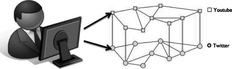
Overlaying social networks. Interactions on YouTube give rise to one graph whereas interactions on Twitter give rise to another with a slightly different topology. The vertical lines link users that are the same on both networks. Interpreting both networks as arising from one agent’s interactions may be a useful way to unify online behavior and link it with psychological models of behavior

Conclusions

Computational methods such as natural language processing and graph theory can analyze data acquired through programmatic interfaces to social networking sites to provide a “real-time epidemiology” of drug abuse. Toxicovigilance via social networks will help prepare frontline clinicians to better recognize the appearance and attend to the needs of their communities. Furthermore, graph theory and agent-based modeling be used to make inferences from social media on the structure of networks that spread and consume information about drug abuse. Insights from these methods can help public health officials identify sentiments and community behavior surrounding these drugs of abuse, which may be of assistance in tailoring interventions and campaigns for prevention. These methods, even despite current limitations, offer several advantages over current efforts at drug detection and characterization, and provide a compelling tool for clinicians, administrators, and investigators.

References

- 1.RTI International. (2012). National survey on drug use and health: sample redesign issues and methodological studies. http://www.samhsa.gov/data/NSDUH/NSDUHMethodsSIMS2012.pdf. Accessed 5 Jan 2013 [PubMed]
- 2.Sloboda Z. Changing patterns of “drug abuse” in the United States: connecting findings from macro- and microepidemiologic studies. Subst Use Misuse. 2002;37(8–10):1229–1251. doi: 10.1081/JA-120004181. [DOI] [PubMed] [Google Scholar]
- 3.Descotes J, Testud F. Toxicovigilance: a new approach for the hazard identification and risk assessment of toxicants in human beings. Toxicol Appl Pharmacol. 2005;207(2 Suppl):599–603. doi: 10.1016/j.taap.2005.02.019. [DOI] [PubMed] [Google Scholar]
- 4.Eysenbach G. Infodemiology and infoveillance: framework for an emerging set of public health informatics methods to analyze search, communication and publication behavior on the internet. J Med Internet Res. 2009;11(1):e11. doi: 10.2196/jmir.1157. [DOI] [PMC free article] [PubMed] [Google Scholar]
- 5.McNeil K, Brna PM, Gordon KE. Epilepsy in the twitter era: a need to re-tweet the way we think about seizures. Epilepsy Behav: E&B. 2012;23(2):127–130. doi: 10.1016/j.yebeh.2011.10.020. [DOI] [PubMed] [Google Scholar]
- 6.Boyer EW, Wines JD., Jr Impact of internet pharmacy regulation on opioid analgesic availability. J Stud Alcohol Drugs. 2008;69(5):703–708. doi: 10.15288/jsad.2008.69.703. [DOI] [PMC free article] [PubMed] [Google Scholar]
- 7.Barratt MJ. Silk road: eBay for drugs. Addiction. 2012;107(3):683. doi: 10.1111/j.1360-0443.2011.03709.x. [DOI] [PubMed] [Google Scholar]
- 8.Lange JE, Daniel J, Homer K, Reed MB, Clapp JD. Salvia divinorum: effects and use among YouTube users. Drug Alcohol Depend. 2010;108(1–2):138–140. doi: 10.1016/j.drugalcdep.2009.11.010. [DOI] [PubMed] [Google Scholar]
- 9.Cavnar WB, and Trenkle JM (1994). N-gram based text categorization. Proc. of SDAIR-94, 3rd Annual Symposium on Document Analysis and Information Retrieval, pp. 161–175
- 10.Ziv J, Lempel A. A universal algorithm for sequential data compression. IEEE Trans Inf Theory. 1977;23(3):337–343. doi: 10.1109/TIT.1977.1055714. [DOI] [Google Scholar]
- 11.Hu J, Gao J, Principe JC. Analysis of biomedical signals by the Lempel–Ziv complexity: the effect of finite data size. IEEE Trans Biomed Eng. 2006;53(12 Pt 2):2606–2609. doi: 10.1109/TBME.2006.883825. [DOI] [PubMed] [Google Scholar]
- 12.Hastie T, Tibshirani R, Friedman J. The elements of statistical learning: data mining, inference, and prediction. 2. New York: Springer; 2009. [Google Scholar]
- 13.Dumais S. Latent semantic analysis. Annu Rev Inf Sci Technol. 2005;38:188. doi: 10.1002/aris.1440380105. [DOI] [Google Scholar]
- 14.Davis ME, Sigal R, Weyuker EJ. Computability, complexity, and languages: fundamentals of theoretical computer science. Boston: Academic; 1994. [Google Scholar]
- 15.Bondy J, Murty U. Graph theory. Graduate texts in mathematics. 3. Springer: New York; 2008. [Google Scholar]
- 16.Watts DJ, Strogatz SH. Collective dynamics of ‘small-world’ networks. Nature. 1998;393(6684):440–442. doi: 10.1038/30918. [DOI] [PubMed] [Google Scholar]
- 17.Cha M. The world of connections and information flow in Twitter. IEEE Trans Syst Man Cybern. 2012;42(4):991–998. doi: 10.1109/TSMCA.2012.2183359. [DOI] [Google Scholar]
- 18.Graham RL, Groetschel M, Lovasz L, editors. Handbook of combinatorics, vols 1 and 2. Amsterdam: Elsevier; 1996. [Google Scholar]
- 19.Schrodinger E (1944). What is life? The physical aspect of the living cell. Dublin: e Dublin Institute for Advanced Studies at Trinity College
- 20.Macklem PT. Emergent phenomena and the secrets of life. J Appl Physiol. 2008;104(6):1844–1846. doi: 10.1152/japplphysiol.00942.2007. [DOI] [PubMed] [Google Scholar]