Sparsity-Based Deconvolution of Low-Dose Perfusion CT Using Learned Dictionaries

Abstract

Computational tomography perfusion (CTP) is an important functional imaging modality in the evaluation of cerebrovascular diseases, such as stroke and vasospasm. However, the post-processed parametric maps of blood flow tend to be noisy, especially in low-dose CTP, due to the noisy contrast enhancement profile and the oscillatory nature of the results generated by the current computational methods. In this paper, we propose a novel sparsity-base deconvolution method to estimate cerebral blood flow in CTP performed at low-dose. We first built an overcomplete dictionary from high-dose perfusion maps and then performed deconvolution-based hemodynamic parameters estimation on the low-dose CTP data. Our method is validated on a clinical dataset of ischemic patients. The results show that we achieve superior performance than existing methods, and potentially improve the differentiation between normal and ischemic tissue in the brain.

1 Introduction

Stroke is the third-leading cause of death in the United States after heart disease and cancer. Early and rapid diagnosis of stroke can save critical time for thrombolytic therapy. Cerebral perfusion imaging via computed tomography perfusion (CTP) has become more commonly used in clinical practice for the evaluation of patients with acute stroke and vasospasm. Various mathematical models have been used to process the acquired temporal data to ascertain quantitative information, such as cerebral blood flow (CBF), cerebral blood volume (CBV) and mean transit time (MTT) [1–3]. However recent reports on over-exposure of radiation in CTP have brought the dosage problem to the limelight because many patients reported biologic effects from radiation exposure, including hair loss and skin burns. A key challenge in CTP is to obtain a high-quality CBF image from a low-dose perfusion scan.

The most commonly used deconvolution method to quantify the perfusion parameters in CTP is truncated singular value decomposition (TSVD) and its variants, such as circular TSVD (cTSVD) [2]. The oscillatory nature [4] of the TSVD-based method has initiated research that incorporates different regularization methods to stabilize the deconvolution, and have shown varying degrees of success in recovering the residue function or the perfusion parameters [3][5–8]. However, prior studies have focused exclusively on imposing regularizations on the noisy low-dose CTP, without considering the corpus of high-dose CTP data.

In this paper, we propose a new sparsity-based deconvolution method to estimate cerebral blood flow in CTP at low-dose. We first learned a dictionary of CBF maps from a corpus of high-dose CTP data and then performed deconvolution-based hemo-dynamic parameter estimation of the low-dose CTP. This method produces perfusion parameter maps with better signal-to-noise characteristics.

Our major contribution in this work is two-fold: First, we propose to train a dictionary of perfusion parameter maps from the high-dose CT data to improve the quantification of low-dose CT perfusion. Second, we use local sparsity and redundancy in a global spatial Bayesian objective combined with the temporal convolution model. Then on the in vivo brain ischemic stroke CTP data, we demonstrate that our estimated CBF values lead to better separation between ischemic tissue—which by its angiogenic nature tends to have less blood flow—and normal tissue.

2 A Dictionary Approach to Deconvolution

In this section, we present the new sparsity based deconvolution framework for CTP quantification. The framework is comprised of two steps: dictionary learning and sparse coding.

2.1 Perfusion Parameter Model

Based on the theoretical model provided in [1], in CTP, the amount of contrast in the region is characterized by

$$C_v(t)=\mathit{CBF}{\int }_0^t{C}_a(\tau )R(t-\tau )d\tau$$ (1)

where C_v(t) is the tissue enhancement curve (TEC) of tracer at the venous output in the volume of interest (VOI), CBF is the cerebral blood flow, C_a(t) is an arterial input function (AIF) and R(t)is the tissue impulse residue function (IRF), which measures the mass of contrast media remaining in the given vascular network over time. To discretize the computation, we assume that C_a(t) and C(t) are measured with N equally spaced time points t₁,t₂,…,t_N, with time increment Δt. The convolution is discretized

$$\mathit{C}=\mathit{CBF}·\mathrm{\Delta }t·{\mathit{C}}_{\mathit{a}}·\mathit{R}$$ (2)

where

$$\mathit{C}=\left(\begin{array}{c}C(t_1)\\ C(t_2)\\ ⋮\\ C(t_N)\end{array}\right)\mathit{R}=\left(\begin{array}{c}R(t_1)\\ R(t_2)\\ ⋮\\ R(t_N)\end{array}\right){\mathit{C}}_{\mathit{a}}=\left(\begin{array}{cccc}{C}_a(t_1)& 0& \cdots & 0\\ C_a(t_2)& C_a(t_1)& \cdots & 0\\ ⋮& ⋮& \ddots & ⋮\\ C_a(t_N)& C_a(t_{N-1})& \cdots & C_a(t_1)\end{array}\right)$$

When R(t) is estimated from Equation (2), CBF can be computed from

$$\mathit{CBF}=R(t=0)$$ (3)

since from the definition of the residue function R(t), R(t=0) =1.

2.2 Proposed Dictionary Learning Approach to Deconvolution

Sparse representations over trained dictionaries for perfusion parameter maps restoration rest on the assumption that the image priors in the perfusion maps can be learned from images, rather than choosing a prior based on some simplifying assumptions, such as spatial smoothness, non-local similarity, or sparsity in the transformed domain. Since the low dose CTP have high noise level in TEC, it is important to learn the dictionaries from the high-dose (thus low noise level) CTP. Therefore, we implement the sparse and redundant representation in the spirit of Sparseland [9]. In our model, we estimate perfusion parameters by considering both temporal correlations and example-based restoration based on dictionaries learned from high-dose data.

Problem Formulation

Suppose C(x,y,z,t) ∈ ℝ^N×T is TEC in VOI [x,y,z]^T from a spatial-temporal patch of size $\sqrt{N}\times \sqrt{N}\times 1$ pixels and T time points. R(x,y,z,t) ∈ ℝ^N×T represent the remaining tracer concentration (RIF) of the voxel [x,y,z] at a given time point t, where x, y and z are the respective row, column and slice coordinates of the spatial-temporal data. The least-square form of (2) is

$$J_{ls}={\left|\right|\mathit{C}-{\mathit{C}}_{\mathit{a}}\mathit{R}\left|\right|}_2^2$$ (4)

Due to the noise in the low-dose CTP data, the solution of (4) may be severely distorted. In the spirit of Sparseland model, we incorporate a prior of not only temporal correlation but also sparse representation from the learned dictionaries of the parameter map patches through the inclusion of two constraints to the original least-square cost function. This results in the new cost function

$$J={\mu }_1{\left|\right|\mathit{C}-{\mathit{C}}_{\mathit{a}}\mathit{R}\left|\right|}_2^2+{\left|\right|x-\mathit{D}\alpha \left|\right|}_2^2+{\mu }_2{\left|\right|\alpha \left|\right|}_0$$ (5)

where x ∈ ℝ^N is the CBF perfusion map we want to estimate for the VOI at [x,y,z], D ∈ ℝ^N×K is the learned dictionary of CBF perfusion map patches that consists of K key patches from the training data. α ∈ ℝ^K represents a sparse vector so that Dα can approximate x with certain error tolerance. From the definition of the residue function, we can get x =R(t = 0). The choice of two parameters μ₁ and μ₂ dictate how important the temporal correlation term (the first term) and the sparsity term (the third term) should be weighted.

Dictionary Learning

To solve D, we use the recently developed K-SVD algorithm [10] which solves (5) by iterating exact K times of Singular Value Decomposition (SVD). We first learn a dictionary by using randomly sampled patches from the CBF perfusion maps estimated from the high-dose CTP data. Given a set of image patches $Z={\{z_j\}}_{j=1}^M$, each of $\sqrt{N}\times \sqrt{N}\times 1$. We seek the dictionary D that minimizes

$${min}_{\mathit{D},\mathit{A}}{\sum }_{j=1}^M{\left|\right|{\alpha }_j\left|\right|}_0,\text{subject}\text{to}{\left|\right|z_j-\mathit{D}{\alpha }_j\left|\right|}_2\le \epsilon ,i=1,\dots ,N$$ (6)

where ε>0 is the prescribed error tolerance of representation error.

To solve (6), we start from an initial dictionary (i.e. the overcomplete DCT dictionary), and an initial estimation of the CBF parameter map (i.e. CBF map from cTSVD algorithm). Then K-SVD algorithm approaches the solution of (6) by alternating the following two steps: the minimization with respect to α with D fixed using orthogonal matching pursuit (OMP), and the update of atoms in D using the current A. The update stage modifies the atoms in D one by one to better represent the data Z. For each column k = 1,2,…,K, we find the index set I_k = {i: α_ki ≠ 0}, which is the set of indices of (z_j’s who used d_k in representation in the sparse coding step. Then we set error matrix E_k = Z_k − D_kA_k, where D_k is D with d_k replaced by 0. Z_k and A_k collect the columns with indices in I_k from Z and A. Finally, we apply SVD decomposition E_k = UΛV^T. Update d_k in D with the first column of U, and the coefficients in α_i. with the entries in V multiplied by Λ(1,1). Theoretically K-SVD solver may not produce stable results, while in this specific application and in all experimental the solver works very well and yields stable reconstructed images.

Sparse Perfusion Deconvolution (SPD)

When the dictionary D is known, the CBF perfusion parametric map from the low-dose CTP data can be estimated using our sparse perfusion deconvolution method by minimizing (5) in an iterative fashion. Our SPD method also consists of iterating the following two steps: minimization with respect to α with x fixed, and update of x with α fixed.

The first step is sparse coding, which is formulated a

$${min}_{{\alpha }_i}{\left|\right|{\alpha }_i\left|\right|}_0,\text{subject}\text{to}{\left|\right|x-\mathit{D}\alpha \left|\right|}_2\le \epsilon$$ (7)

where the value of ε implies specific value for μ₂. Equation (7) can be solved by any matching pursuit algorithm. Here we use orthogonal matching pursuit (OMP).

The second step is to minimize

$${min}_x{\mu }_1{\left|\right|\mathit{C}-{\mathit{C}}_{\mathit{a}}\mathit{R}\left|\right|}_2^2+{\left|\right|x-\mathit{D}\alpha \left|\right|}_2^2$$ (8)

Because x = R(t = 0), (8) can be rewritten as

$${min}_x{\mu }_1{\left|\right|\mathit{C}-{\mathit{C}}_{\mathit{a}}\widehat{\mathit{R}}·\mathit{diag}(x)\left|\right|}_2^2+{\left|\right|x-\mathit{D}\alpha \left|\right|}_2^2$$ (9)

where R̂ is the residue functions normalized by x so that R̂(t = 0) = 1. (9) is a quadratic term that has a closed-form solution.

If vec(B) denotes the vector formed by the entries of a matrix B in column major order, and define P = C_aR̂, then

$$\text{vec}\left(\mathit{C}-{\mathit{C}}_{\mathit{a}}\widehat{\mathit{R}}·\mathit{diag}(x)\right)=\text{vec}\left(\mathit{C}-\mathit{P}·\text{diag}(x)\right)=\text{vec}(\mathit{C})-\mathit{M}x$$ (10)

where M is a TN × N matrix in form of

$$\mathit{M}=\left(\begin{array}{cccc}{P}_{.,1}& 0& \cdots & 0\\ 0& P_{.,2}& \cdots & 0\\ ⋮& ⋮& \ddots & ⋮\\ 0& 0& \cdots & P_{.,N}\end{array}\right)$$

where P_.,i. dictates the i^th column of matrix P in its column vector form. Equation (9) can be transformed into the conventional least square problem

$${min}_x{\left|\right|({\mathit{I}}_{\mathit{n}};\mathit{M})x-[\mathit{D}a;\text{vec}(\mathit{C})]\left|\right|}_2^2$$ (11)

Let A= (I_n;M). and B = (Dα;vec(C)), we get

$$x={\mathit{A}}^{+}\mathit{B}$$ (12)

where A⁺. is the pseudo-inverse of matrix A, (.;,) denotes a vector or matrix by stacking the arguments vertically.

To address the global CBF deconvolution problem, we use a sliding window of size $\sqrt{N}\times \sqrt{N}$ on the specific slice and overlaps the windows by step size of 1. The final global CBF parametric map is generated by averaging the areas that the windows overlap.

3 Experiments

In this section, we describe the results from comparing our approach with cTSVD on four clinical subjects with ischemia related to vasospasm. The presence and location of the perfusion deficits were identified by board-certified radiologists with subspecialty training in neuroradiology.

3.1 Data Acquisition

CTP was performed during the typical time-period for vasospasm in aneurysmal sub-arachnoid hemorrhage, between days 6–8 in asymptomatic patients and on the same day clinical deterioration occurred in symptomatic patients. There is a standard scanning protocol for CTP at our institution using GE Lightspeed or Pro-16 scanners (General Electric Medical Systems, Milwaukee, WI) with cine 4i scanning mode and 45 second acquisition at 1 rotation per second using 80 kVp and 190 mA.

3.2 Experimental Results

For cTSVD, a threshold of 6% of the maximum singular value is used, in accordance with parameter tuning in our experiments. For all experiments, the dictionary used are of size 64×256, designed to handle perfusion image patches of 8×8 pixels. In all experiments, the denoising process uses a sparse coding of each patch of size 8×8 pixels from noisy image. The parameters are chosen empirically and the experimental results are not sensitive to the parameters. Repetitive scanning of the same patient at different radiation doses is unethical and a physiological phantom which can uptake contrast agent is currently not available. Thereby, low-dose CTP data is simulated following the practice in [11], where Gaussian noise ε~N(0,σ²) is added to the high-dose CTP data. In the following, peak signal-to-noise ratio (PSNR) is calculated by dividing the peak value of the tissue time-enhancement curve by the noise standard deviation σ.

1) Learned Dictionaries

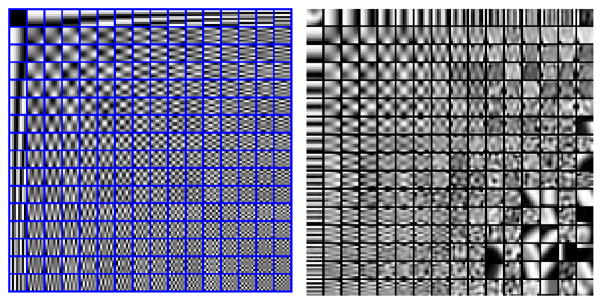
Figure 1 shows the redundant DCT dictionary on the left, with each atom of an 8×8 pixel image. This dictionary was used as the initialization for the training. The globally trained dictionary is shown on the right side of Fig. 1. This dictionary was trained on a data-set of 10,000 8×8 patches of high-dose CBF perfusion maps.

Fig. 1.

Left: DCT dictionary. Right: Globally trained dictionary using high-dose CBF maps.

2) LACA Estimation

Figure 2 shows CBF maps and the zoomed-in regions of a normal clinical subject. The zoomed-in region of the left anterior cerebral artery (LACA) territory (in X-ray image left and right are opposite) of the CBF map using TSVD in high-dose (190mA), low-dose (PSNR=20) and using SPD in low-dose (PSNR=20) are shown on the right. The vascular region supplied by the LACA has increased noise in the CBF map using TSVD.

Fig. 2.

(a) An acquired CT image from a CTP exam in a normal subject. (b) Left anterior cerebral artery (LACA) territory using cTSVD in high-dose (190mA) (c) cTSVD in low-dose (PSNR=20) (d) our proposed SPD in low-dose (PSNR=20) data.

In comparison, significantly improved spatial smoothness in the vascular region and higher color contrast between the artery region and the vascular region can be observed from the CBF map computed using our proposed method. The standard deviation the LACA region computed using TSVD and SPD under different PSNR are shown in Table 1.

Table 1.

Standard deviation of the LACA region on a patient with normal blood flow under different PSNR using TSVD and our SPD method.

PSNR	20	40	60	80
TSVD	56.09	47.11	23.14	22.98
SPD	41.94	42.12	16.44	16.47

3) Ischemic Comparison

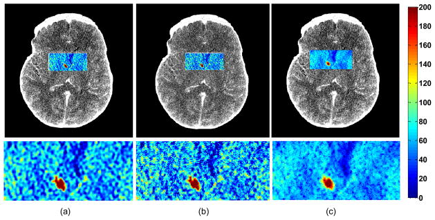
We also show the CBF maps processed for patients with ischemic deficits (Figure 3) using TSVD and our proposed SPD on high-dose and low-dose CTP data. On the left, the low value of CBF in the ischemic patient becomes more evident while the vascular regions become smoother and variations in the estimated blood flow maps are reduced greatly by our method. The difference of the blood flows between the vascular and the artery regions were significantly enlarged.

Fig. 3.

CBF maps and zoomed-in regions in an ischemic patient with a RMCA deficit estimated by (a) TSVD in high-dose (b) TSVD in low-dose (c) SPD in low-dose. Low blood flow is delineated in blue. Red color indicates high blood flow value, while blue color indicates low blood flow value.

4) Ischemic Voxels Clustering

By aggregating all voxels (within the VOI) from the normal patient data sets into a single “normal” group with n₁ samples, and the ischemia patient data sets into an “abnormal” group with n₂ samples. In our case, n₁=1000 and n₂=1000. To quantify the separability between normal and ischemic CBF values, we define the distance between these two clusters as:

$$d=\frac{{\mu }_1-{\mu }_2}{\sqrt{{\sigma }_1^2/n_1+{\sigma }_2^2/n_2}}$$ (13)

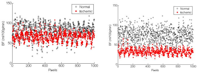
where μ₁, μ₂ are the means, and σ₁, σ₂ are the standard deviations of CBF in the normal and ischemic clusters respectively. We expect our SPD algorithm to produce larger distance d as defined in Eq. (13), that is, to more definitely differentiate between normal and ischemic regions in the brain. Fig. 4 show scatter plots of normal vs. ischemic clusters. It is apparent that the two clusters are more separable in data processed via SPD than TSVD.

Fig. 4.

(a) Two clusters of normal vs. ischemic regions in the brain generated by TSVD method. The distance d between two clusters is 22.67. (b) Two clusters of normal vs. ischemic regions by our sparse perfusion deconvolution method. The distance d between two clusters is 63.79.

4 Conclusion

In this paper, we introduced a novel sparsity-based deconvolution algorithm to estimate cerebral blood flow in low-dose CTP. We trained a dictionary using CBF maps computed from high-dose CTP and then performed deconvolution-based hemodynamic parameter estimation of the low-dose CTP data. The experimental results indicated that our algorithm not only outperforms TSVD algorithm but also may significantly improve the diagnostic performance of ischemia related to vasospasm in aneurysmal subarachnoid hemorrhage patients.

References

- 1.Østergaard L, Weisskoff RM, Chesler DA, Gyldensted C, Rosen BR. High Resolution Measurement of Cerebral Blood Flow Using Intravascular Tracer Bolus Passages. Part I: Mathematical Approach and Statistical Analysis. Magn Reson Med. 1996;36:715–725. doi: 10.1002/mrm.1910360510. [DOI] [PubMed] [Google Scholar]
- 2.Wittsack HJ, Wohlschlager A, Ritzl E, Kleiser R, Cohnen M, Seitz R, Moder U. CT-Perfusion Imaging Of The Human Brain: Advanced Deconvolution Analysis Using Circulant Singular Value Decomposition. Computerized Med Imag Graphics. 2008;32:67–77. doi: 10.1016/j.compmedimag.2007.09.004. [DOI] [PubMed] [Google Scholar]
- 3.He L, Orten B, Do S, Karl WC, Kambadakone A, Sahani DV, Pien H. A Spatio-Temporal Deconvolution Method To Improve Perfusion CT Quantification. IEEE Transactions on Medical Imaging. 2010;29(5):1182–1191. doi: 10.1109/TMI.2010.2043536. [DOI] [PubMed] [Google Scholar]
- 4.Mouridsen K, Friston K, Hjort N, Gyldensted L, Ostergaard L, Kiebel S. Bayesian estimation of cerebral perfusion using a physiological model of microvasculature. Neuro Image. 2006;33:570–579. doi: 10.1016/j.neuroimage.2006.06.015. [DOI] [PubMed] [Google Scholar]
- 5.Pack N, DiBella E, Rust T, Kadrmas D, McGann C, Butterfield R, Christian P, Hoffman J. Estimating Myocardial Perfusion From Dynamic Contrast-Enhanced CMR With A Model-Independent Deconvoution Method. J Cardiovas Magn Reson. 2008;10:52. doi: 10.1186/1532-429X-10-52. [DOI] [PMC free article] [PubMed] [Google Scholar]
- 6.Wong K, Tam C, Ng M, Wong S, Young G. Improved Residue Function and Reduced Flow Dependence In MR Perfusion Using Least-Absolute-Deviation Regularization. Magn Reson Med. 2009;61:418–428. doi: 10.1002/mrm.21860. [DOI] [PubMed] [Google Scholar]
- 7.Fang R, Chen T, Sanelli PC. Sparsity-Based Deconvolution of Low-dose Brain Perfusion CT in Subarachnoid Hemorrhage Patients. IEEE Proceedings of theNinth International Symposium on Biomedical Imaging. 2012 [Google Scholar]
- 8.Fang R, Raj A, Chen T, Sanelli PC. Radiation Dose Reduction In Computed Tomography Perfusion Using Spatial-Temporal Bayesian Methods. In: Pelc NJ, Nishikawa RM, Whiting BR, editors. Medical Imaging, SPIE. Vol. 8313. 2012. pp. 45–53. [Google Scholar]
- 9.Elad M, Aharon M. Image Denoising Via Sparse And Redundant Representations Over Learned Dictionaries. IEEE Transactions On Image Processing. 2006;15(12) doi: 10.1109/tip.2006.881969. [DOI] [PubMed] [Google Scholar]
- 10.Aharon M, Elad M, Bruckstein A, Katz Y. K-SVD: An Algorithm for Designing of Overcomplete Dictionaries for Sparse Representation. IEEE Transactions on Signal Processing. 2006;54:4311–4322. [Google Scholar]
- 11.Britten A, Crotty M, Kiremidjian H, Grundy A, Adam E. The Addition Of Computer Simulated Noise To Investigate Radiation Dose And Image Quality in Images with Spatial Correlation Of Statistical Noise: An Example Application To X-Ray CT Of The Brain. British Journal of Radiology. 2004;77(916):323. doi: 10.1259/bjr/78576048. [DOI] [PubMed] [Google Scholar]