Predicting catastrophes in nonlinear dynamical systems by compressive sensing

Abstract

An extremely challenging problem of significant interest is to predict catastrophes in advance of their occurrences. We present a general approach to predicting catastrophes in nonlinear dynamical systems under the assumption that the system equations are completely unknown and only time series reflecting the evolution of the dynamical variables of the system are available. Our idea is to expand the vector field or map of the underlying system into a suitable function series and then to use the compressive-sensing technique to accurately estimate the various terms in the expansion. Examples using paradigmatic chaotic systems are provided to demonstrate our idea and potential challenges are discussed.

It has been recognized that nonlinear dynamics are ubiquitous in many natural and engineering systems. A nonlinear system, in its parameter space, can often exhibit catastrophic bifurcations that ruin the desirable or ’normal” state of operation. Consider, for example, the phenomenon of crisis [1] where, as a system parameter is changed, a chaotic attractor collides with its own basin boundary and is suddenly destroyed. After the crisis, the state of the system is completely different from that on the attractor before the crisis. Suppose that, for a nonlinear dynamical system, the state before the crisis is normal and desirable, and the state after the crisis is undesirable or destructive. The crisis can thus be regarded as a catastrophe that one strives to avoid at all cost. Catastrophic events, of course, can occur in different forms in all kinds of natural and man-made systems. A question of paramount importance is how to predict catastrophes in advance of their possible occurrences. This is especially challenging when the equations of the underlying dynamical system are unknown and one must then rely on measured time series or data to predict any potential catastrophe.

In this paper, we articulate a strategy to address the problem of predicting catastrophes in nonlinear dynamical systems. We assume that an accurate model of the system is not available, i.e., the system equations are unknown, but the time evolutions of the key variables of the system can be accessed through monitoring or measurements. Our method consists of three steps: (i) predicting the dynamical system based on time series, (ii) identifying the parameters of the system, and (iii) performing bifurcation analysis using the predicted system equations to locate potential catastrophic events in the parameter space so as to determine the likelihood of system’s drifting into a catastrophe regime. In particular, if the system operates at a parameter setting close to such a critical bifurcation, catastrophe is imminent as a small parameter change or a random perturbation can push the system beyond the bifurcation point. To be concrete, in this paper we regard crises as catastrophes. Once a complete set of system equations has been predicted and the parameters have been identified, one needs to examine the available parameter space. In general, to explore the multi-parameter space of a dynamical system can be extremely challenging, which can often lead to the discovery of new phenomena in dynamics. An early example in this area of research is the work by Stewart et al. [2], which investigated the phenomenon of double crises in two-parameter dynamical systems. More recent efforts include the investigation of hierarchical structures in the parameter space [3]. The present focus of our work, however, is on predicting the dynamical systems based on compressive sensing.

The problem of predicting dynamical systems based on time series has been outstanding in nonlinear dynamics because, despite previous efforts [4] in using the standard delay-coordinate embedding method [5] to decode the topological properties of the underlying system, how to accurately infer the underlying nonlinear system equations remains largely an unsolved problem. In principle, a nonlinear system can be approximated by a large collection of linear equations in different regions of the phase space, which can indeed be achieved by reconstructing the Jacobian matrices on a proper grid that covers the phase-space region of interest [6, 7]. However, the accuracy and robustness of the procedure are challenging issues, including the difficulty with the required computations. In order to be able to predict potential catastrophes, local reconstruction of a large set of linearized dynamics is not sufficient but rather, an accurate prediction of the underlying non-linear equations themselves is needed.

Our framework to fully reconstruct dynamical systems using time series alone is based on the assumption that the dynamics of many natural and man-made systems are determined by functions that can be approximated by series expansions in a suitable base. The major task is then to estimate the coefficients in the series representation. In general, the number of coefficients to be estimated can be large but many of them are zero (the sparsity condition). According to the conventional wisdom this would be a difficult problem as a large amount of data is required and the computations involved can be extremely demanding. However, the recent paradigm of compressive sensing developed by Candès et al. [8-11] provides a viable solution to the problem, where the key idea is to reconstruct a sparse signal from small amount of observations [8-11], as measured by linear projections of the original signal on a few predetermined vectors. Since the requirements for the observations can be considerably relaxed as compared with those associated with conventional signal reconstruction schemes, compressive sensing has received much recent attention and it is becoming a powerful technique to obtain high-fidelity signal for applications where sufficient observations are not available. Here, we shall articulate a general methodology to cast the problems of dynamical-system prediction into the framework of compressive sensing and we demonstrate the power of our method by carrying out bifurcation analyses on the predicted dynamical systems to locate potential catastrophes using exemplary chaotic systems.

Generally, the problem of compressive sensing can be described as the reconstruction of a sparse vector a ∈ R^v from linear measurements X about a in the form: X = G·a, where X ∈ R^w, G is a w × v matrix and most components of a are zero. The compressive sensing theory ensures that the number of components of the unknown signal can be much larger than the number of required measurements for reconstruction, i.e., v ≫ w. Accurate reconstruction can be achieved by solving the following convex optimization problem [12]: min ∥a∥₁ subject to G·a = X, where ${\parallel \mathbf{a}\parallel }_1={\sum }_{i=1}^N\mid {\mathbf{a}}_i\mid$ is the L₁ norm of a. Solutions to the convex optimization problem has been worked out recently [12, 13].

We first show that the inverse problem of predicting dynamical systems can be cast in the framework of compressive sensing so that optimal solutions can be obtained even when the number of power-series coefficients to be estimated is large and/or the amount of available data is small. Assume that the dynamical system can generally be written as $\stackrel{.}{\mathbf{x}}=\mathbf{F}\left(\mathbf{x}\right)$, where x ∈ R^m represents the set of externally accessible dynamical variables and F is a smooth vector function in R^m. The jth component of F(x) can be represented, for example, by a power series:

$${\left[\mathbf{F}\right(\mathbf{x}\left)\right]}_j=\sum _{l_1=0}^n\sum _{l_2=0}^n\cdot \sum _{l_m=0}^n{\left[{\mathbf{a}}_j\right]}_{l_1,\cdots ,l_m}\cdot x_1^{l_1}{x}_2^{l_2}\cdots x_m^{l_m},$$ (1)

where x_k (k = 1, ⋯, m) is the kth component of the dynamical variable, the total number of products is (1 + n)^m, and [a_j]_l1,⋯,lm ∈ R^m is the coefficient scalar of each product term to be determined from measurements. Note that the terms in Eq. (1) are all possible products of different components with different powers.

To better explain our method, without loss of generality, we focus on one dynamical variable of the system. (Procedures for other variables are similar.) From Eq. 1, we see that the number of coefficients to be determined is then (n + 1)^m. The vector a to be determined in the compressive-sensing framework contains then (n + 1)^m components. For example, to construct the measurement vector X and the matrix G for the case of m = 3 (dynamical variables x, y, and z) and n = 3, we have the following explicit dynamical equation for the first dynamical variable: ${\left[\mathbf{F}\right(\mathbf{x}\left)\right]}_1\equiv a_{0,0,0}{x}^0{y}^0{z}^0+a_{1,0,0}{x}^1{y}^0{z}^0+\cdots +a_{1,0,3}{x}^1{y}^0{z}^3+\cdots +a_{1,1,0}{x}^1{y}^0{z}^0+\cdots +a_{3,3,3}{x}^3{y}^3{z}^3$. We can denote the coefficients of [F(x)]₁ by $\mathbf{a}={[a_{0,0,0},a_{0,0,1},\cdot ,a_{3,3,3}]}^T$. Assuming that measurements of x(t) at a set of time t₁, t₂, …, t_w are available, we denote $\mathbf{g}\left(t\right)=[x{\left(t\right)}^{0}y{\left(t\right)}^{0}z{\left(t\right)}^0,x{\left(t\right)}^{0}y{\left(t\right)}^{0}z{\left(t\right)}^1,\cdots ,x{\left(t\right)}^{3}y{\left(t\right)}^{3}z{\left(t\right)}^3]$, such that [F(x(t))]₁ = g(t) · a. From the expression of [F(x)]₁, we can choose the measurement vector as $\mathbf{X}={\left[\stackrel{.}{x}\right(t_1),\stackrel{.}{x}(t_2),\cdots ,\stackrel{.}{x}(t_w\left)\right]}^T$, which can be calculated from time series. Finally, we obtain the following equation in the form X = G · a:

$$\left(\begin{array}{c}\hfill \stackrel{.}{x}\left(t_1\right)\hfill \\ \hfill \stackrel{.}{x}\left(t_2\right)\hfill \\ \hfill ⋮\hfill \\ \hfill \stackrel{.}{x}\left(t_w\right)\hfill \end{array}\right)=\left(\begin{array}{c}\hfill \mathbf{g}\left(t_1\right)\hfill \\ \hfill \mathbf{x}\left(t_2\right)\hfill \\ \hfill ⋮\hfill \\ \hfill \mathbf{x}\left(t_w\right)\hfill \end{array}\right)\left(\mathbf{a}\right),$$

where, to ensure the restricted isometry property [12], we normalize it by dividing elements in each column by the L₂ norm of that column: (G)_ij = (G)_ij/L₂(j) with $L_2\left(j\right)=\sqrt{{\sum }_{i=1}^M{\left[{\left(\mathbf{G}\right)}_{ij}\right]}^2}$. After a is determined via some standard compressive-sensing algorithm, the coefficients are given by a/L₂. To determine the set of power-series coefficients corresponding to a different dynamical variable, say y, we simply replace the measurement vector by $\mathbf{X}={\left[\stackrel{.}{y}\right(t_1),\stackrel{.}{y}(t_2),\cdots ,\stackrel{.}{y}(t_w\left)\right]}^T$ and use the same matrix G. This way all coefficients can be estimated.

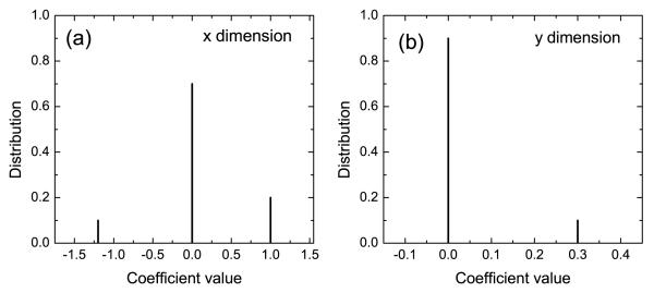
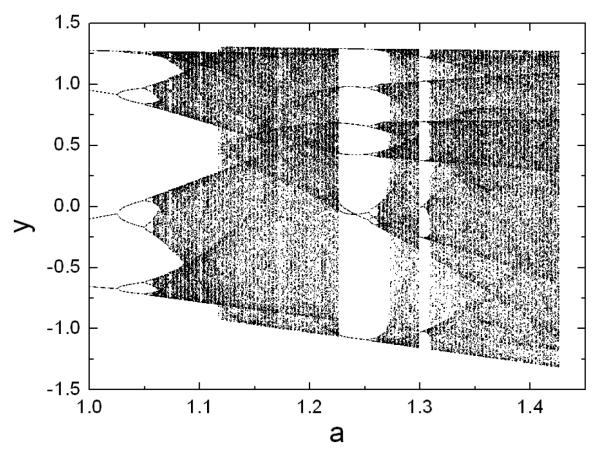
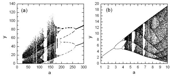
We now present a number of physically relevant examples to illustrate our strategy. The first example is the Hénon map [14], a classical model that has been used to address many fundamental issues in chaotic dynamics. The prediction of map equations resembles that of a vector field. The map is given by: $(x_{n+1},y_{n+1})=(1-a{x}_n^2+y_n,b{x}_n)$, where a and b are parameters. For b = 0.3, the map exhibits periodic and chaotic attractors for a < a_c ≈ 1.42625, where a_c is the critical parameter value for a boundary crisis [1], above which almost all trajectories diverge. The crisis can then be regarded as a catastrophe in the system evolution. Assuming, e.g., that the ’normal” operation of the system corresponds to a chaotic attractor, we choose a = 1.4. Now suppose that the system operates at this parameter value and the system equations are completely unknown but the time series ({x}_n, {y}_n) can be obtained in real time. The goal is to assess, based on the time series only, how ’close” the system is to a potential catastrophe. (If measurements of only one dynamical variable can be obtained, one has to resort to the delay-coordinate embedding method [5].) For illustrative purpose, we assume power-series expansions up to order 3 in the map equations. Figure 1 shows the distributions of the estimated power-series coefficients, where we observe extremely narrow peaks about zero, indicating that a large number of the coefficients are effectively zero, which correspond to nonexistent terms in the map equations. Coefficients that are not included in the zero peak correspond then to existent terms and they determine the predicted map equations. Figures 2 shows the bifurcation diagram from the predicted Hénon map, which is consistent with the original diagram impressively well. In particular, the predicted system gives the value of the critical bifurcation point to within 10⁻³, where a boundary crisis occur. Note that, to predict correctly the map equations, the number of required data is extremely low, not seen before in any method of dynamical-system reconstruction. Similar results have been obtained for the chaotic Lorenz [15] and Rössler [16] oscillators, as shown by the predicted bifurcation diagrams in Figs. 3(a) and (b), respectively. These agree with the original bifurcation diagrams extremely well, so that all possible critical bifurcation points can be predicted accurately based on time series only.

FIG. 1.

For the Hénon map, in (a) x dimension and (b) y dimension, distributions of the predicted values of the ten power-series coefficients up to order 3: constant, y, y², y³, x, xy, xy², x², x²y and x³.

FIG. 2.

Bifurcation diagrams of the predicted Hénon map. The predicted map equations are: $x_{n+1}=0.999999996105743+1.000000008610316\times y_n-a{x}_n^2$ and y_n+1 = 0.29999999837 × x_n. The number n_m of measurements used for prediction is 8 and the total number n_nz + n_z of terms to be predicted is 16.

FIG. 3.

Bifurcation diagram of (a) the predicted Lorenz system given by $\stackrel{.}{x}=10.000548307148881\times y-10.001897147696283\times x$, $\stackrel{.}{y}=x(a-1.000933186801829\times z)-1.000092963203845\times y$, $\stackrel{.}{z}=0.999893761636553\times xy-2.666477325955504\times z$ and of (b) the predicted Rössler system given by $\stackrel{.}{x}=-0.999959701293536\times y-0.999978902248041\times z$, $\stackrel{.}{y}=1.000004981649221\times x+0.200005996113158\times y$, $\stackrel{.}{z}=0.199997011085648+0.999999156496251\times z(x-a)$. In both cases, n_m = 18 and n_nz + n_z = 35.

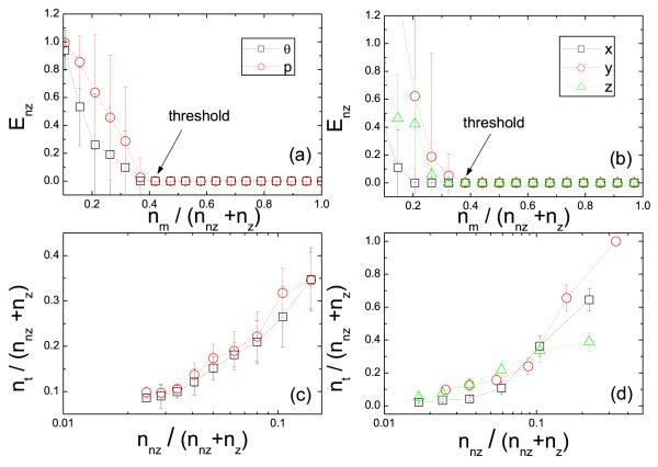
To quantify the performance of our method with respect to the amount of required data, we investigate the prediction errors which are defined separately for nonzero (existing) and zero terms in the dynamical equations. The relative error of a nonzero term is defined as the ratio to the true value of the absolute difference between the predicted and true values. The average over the errors of all terms in a component is the prediction error E_nz of nonzero terms for the component. In contrast, the absolute error E_z is used for zero terms. Figure 4(a) and (b) show E_nz as a function of the ratio of the number n_m of measurements to the total number n_nz + n_z of terms to be predicted, for the standard map [17] and the Lorenz system, respectively. We see that, when the number n_m of measurements exceeds a threshold n_t, E_nz becomes effectively zero. Without loss of generality, we define n_t by using the small threshold value E_nz = 10⁻³ so that n_t is the minimum number of required measurements for an accurate prediction. In Figs. 4(a) and 4(b), we observe that n_t is much less than n_nz + n_z if n_nz, the number of nonzero terms, is small. The performance of our method can thus be quantified by the threshold with respect to the numbers of measurements and terms to be predicted. As shown in Figs. 4(c) and 4(d) for the standard map and the Lorenz system, respectively, as the nonzero terms become sparser among all terms to be predicted (characterized by a decrease in n_nz/(n_nz + n_z) when n_nz + n_z is increased), the ratio of the threshold n_t to the total number of terms n_nz + n_z becomes smaller. These results demonstrate the advantage of our compressive-sensing based method to predict dynamical systems, i.e., high accuracy and extremely low required measurements. In general, to predict the nonlinear dynamical system as accurately as possible, many terms should be assumed in the series expansions. This, surprisingly, not only makes the sparsity condition easy to satisfy, but also can help reduce considerably the required amount of data.

FIG. 4.

Prediction errors E_nz in dynamical equations as a function of the ratio of the number n_m of measurements to the total number n_nz + n_z of terms to be predicted for (a) the standard map and (b) the Lorenz system. The ratio of the threshold n_t to n_nz + n_z for different equations as a function of the ratio n_nz/(n_nz + n_z) for (c) the standard map and (d) the Lorenz system. In (a) and (b), n_nz +n_z is 20 and 35, respectively. The error bars represent the standard deviations obtained from 30 independent realizations. For the standard map, trigonometric functions are included in the series expansion. In (c) and (d), n_nz + n_z can be adjusted by the order of power series. In (c), the data points ranges from order 3 to order 11, and in (d) from order 2 to order 7. We find that E_nz and E_z exhibit the same threshold.

In addition, we examine the resistance of the method to measurement errors by inserting noise into time series. The prediction errors as a function of noise amplitude are shown in Figs. 5(a) and 5(b) for the Hénon map and the standard map, respectively. The results demonstrate that our method is robust against noise, due to the optimization nature of the compressive-sensing method.

FIG. 5.

Prediction errors E_nz as a function of noise amplitude for (a) the Hénon map and (b) the standard map. Uniform noise is added to the time series. The values of n_m and n_nz + n_z for (a) are 8 and 16, respectively, and for (b) are 10 and 20, respectively. The prediction errors in the zero terms show similar behaviors.

There are also situations where the system is high-dimensional or stochastic, for which the current method may not work. A possible solution is to employ the Bayesian inference to determine the system equations. In general the computational challenge associated with the approach can be formidable, but the compressive-sensing method articulated in this paper may present an effective strategy to overcome the difficulty.

In summary, we have articulated a general approach to predicting catastrophes in nonlinear dynamical systems. Our idea is to approximate the equations of the underlying system by series expansion and then to formulate the problem of estimating the various terms in the expansions using compressive sensing. The merit of our approach is then that, due to the nature of the compressive-sensing method, a large number of terms can be accurately estimated even with short available time series, enabling potential implementation in real times. We have presented a number of examples from chaotic dynamics to demonstrate the effectiveness of our method. Predicting catastrophe is a problem of uttermost importance in science and engineering and of extremely broad interest as well, and we hope our work will stimulate further efforts in this challenging area.

References

- [1].Grebogi C, Ott E, Yorke JA. Phys. Rev. Lett. 1982;48:1507. and Physica D. 1983;7:181.
- [2].Stewart HB, Ueda Y, Grebogi C, Yorke JA. Phys. Rev. Lett. 1995;75:2478. doi: 10.1103/PhysRevLett.75.2478. [DOI] [PubMed] [Google Scholar]
- [3].Bonatto C, Gallas JA. Phys. Rev. Lett. 2008;101:054101. doi: 10.1103/PhysRevLett.101.054101. [DOI] [PubMed] [Google Scholar]; Stoop R, Benner P, Uwate Y. Phys. Rev. Lett. 2010;105:074102. doi: 10.1103/PhysRevLett.105.074102. [DOI] [PubMed] [Google Scholar]
- [4].Kantz H, Schreiber T. Nonlinear Time Series Analysis. Cambridge University Press; Cambridge, UK: 1997. [Google Scholar]
- [5].Takens F. Dynamical Systems and Turbulence. In: Rand DA, Young L-S, editors. Lecture Notes in Mathematics. Vol. 898. Springer-Verlag; New York: 1981. pp. 366–381. [Google Scholar]
- [6].Doyne Farmer J, Sidorowich JJ. Phys. Rev. Lett. 1987;59:845. doi: 10.1103/PhysRevLett.59.845. [DOI] [PubMed] [Google Scholar]
- [7].Sauer TD. Phys. Rev. Lett. 2004;93:198701. doi: 10.1103/PhysRevLett.93.198701. [DOI] [PubMed] [Google Scholar]
- [8].Candès E. Proceedings of the International Congress of Mathematicians; Madrid, Spain. 2006. [Google Scholar]
- [9].Baraniuk RG. IEEE Signal Processing Mag. 2007;24:118. [Google Scholar]
- [10].Candès E, Wakin M. IEEE Signal Processing Mag. 2008;25:21. [Google Scholar]
- [11].Romberg J. IEEE Signal Processing Mag. 2008;25:14. [Google Scholar]
- [12].Candès E, Romberg J, Tao T. IEEE Trans. Inf. Theory. 2006;52:489. [Google Scholar]; Commun. Pure Appl. Math. 2006;59:1207. [Google Scholar]
- [13].Candès E, Romberg J. 2005 http://www.acm.caltech.edu/l1magic.
- [14].Hénon M. Commun. Math. Phys. 1976;50:69. [Google Scholar]
- [15].Lorenz EN. J. Atmos. Sci. 1963;20:130. [Google Scholar]
- [16].Rössler OE. Phys. Lett. A. 1976;57:397. [Google Scholar]
- [17].Chirikov BV. Phys. Rep. 1979;52:263. [Google Scholar]