Mediation analysis allowing for exposure-mediator interactions and causal interpretation: theoretical assumptions and implementation with SAS and SPSS macros

Abstract

Mediation analysis is a useful and widely employed approach to studies in the field of psychology and in the social and biomedical sciences. The contributions of this paper are several-fold. First we seek to bring the developments in mediation analysis for non linear models within the counterfactual framework to the psychology audience in an accessible format and compare the sorts of inferences about mediation that are possible in the presence of exposure-mediator interaction when using a counterfactual versus the standard statistical approach. Second, the work by VanderWeele and Vansteelandt (2009, 2010) is extended here to allow for dichotomous mediators and count outcomes. Third, we provide SAS and SPSS macros to implement all of these mediation analysis techniques automatically and we compare the types of inferences about mediation that are allowed by a variety of software macros.

Introduction

Mediation analysis investigates the mechanisms that underlie an observed relationship between an exposure variable and an outcome variable and examines how they relate to a third intermediate variable, the mediator. Rather than hypothesizing only a direct causal relationship between the independent variable and the dependent variable, a mediational model hypothesizes that the exposure variable causes the mediator variable, which in turn causes the outcome variable. The mediator variable then serves to clarify the nature of the relationship between the exposure and outcome variable (MacKinnon, 2008). For example, it might be of interest to understand whether a rehabilitation program for drug-addicted individuals, with methadone as treatment, leads to increased work activity and whether drug use may mediate some of this effect. In this example, drug use may be a potential mediator of the relationship between the methadone treatment and the work activity outcome since the level of methadone may affect drug use, which may in turn affect work activity.

The use of mediation analysis in psychology and in the social sciences is widespread and has been strongly influenced by the seminal paper of Baron and Kenny (1986). More recently, new advances in mediation analysis have been made by using the counterfactual framework (Robins and Greenland, 1992; Pearl, 2001; VanderWeele and Vansteelandt, 2009, 2010; Imai et al., 2010a b). Using the counterfactual framework has allowed for definitions of direct and indirect effects and for decomposition of a total effect into direct and indirect effects even in models with interactions and non-linearities. In many contexts investigators are interested in assessing whether most of the effect is mediated through a particular intermediate or the extent to which it is through other pathways. Decomposition of a total effect into direct and indirect effects accomplishes this goal.

It is then possible to use this counterfactual framework to extend formulae from Baron and Kenny (1986) to allow for mediation analysis even in the presence of exposure mediator interactions. Special cases for mediated effects in the presence of interaction have appeared previously in the literature (e.g. Preacher et al., 2007) but do not give definitions of direct effects such that the total effect decomposes into a direct and indirect effect. In particular, VanderWeele and Vansteelandt (2009, 2010) derived results for direct and indirect effects for linear and logistic regressions when exposure-mediator interaction is present. In many studies it is unrealistic to assume that the exposure and mediator do not interact in their effects on the outcome. Carrying out mediation analysis incorrectly assuming no interaction may result in invalid inferences. The present paper makes a number of important contributions to mediation analysis from both methodological and implementation perspectives. First, we extend work on causal mediation analysis for parametric models with interactions (VanderWeele and Vansteelandt, 2009, 2010) to allow for dichotomous mediators, and not simply continuous mediators as were previously considered. This is done using Pearl’s mediation formula (Pearl, 2001), also described outside the context of counterfactuals elsewhere (Huang et al., 2004). Second, we moreover extend the results to count data. Third, we provide SAS and SPSS macros, which give estimates and confidence intervals for direct and indirect effects when interactions between the mediator of interest and the exposure are present and we compare the types of inference about mediation that are available in a variety of software packages. Finally, we will compare and contrast the inferences that are possible about direct and indirect effects in the presence of exposure-mediator interaction, when using the counterfactual framework versus the traditional statistical approach. We consider both continuous and dichotomous variables as outcomes and mediators and allow for general treatment variables. The approach here enriches the contributions of Baron and Kenny and expands the previous software developed by Preacher and Hayes (2004) and Preacher et al. (2007) to allow for effect decomposition of a total effect into direct and indirect effects in the presence of exposure-mediator interaction and other non-linearities.

The paper is organized as follows. The first section discusses the approach to mediation analysis sometimes referred to as the “product method” and made popular by Baron and Kenny. The second section introduces the reader to the counterfactual approach which gives rise to broader definitions of direct and indirect effects and allows one to carry out mediation analysis and effect decomposition when interaction between exposure and mediator is present. In the following section, conditions are given for the identifiability of direct and indirect effects in mediation analysis; these are the conditions needed for the results of statistical procedures to have a causal interpretation. The next section clarifies the relationship between the results on mediation analysis that arise within the counterfactual framework with other popular approaches to mediation analysis. The paper continues with instructions for using the software developed (SAS and SPSS) and a description of the output is provided. We conclude by providing an example of mediation analysis performed using the mediation macros.

Classic Regression Approach to Mediation Analysis

The practice of mediation analysis in the field of psychology has been highly influenced by the work of Baron and Kenny (1986). The causal diagram in Figure 1 captures how they conceptualized the role of a mediator variable. In this graph, which represents a simple mediation model, A denotes an exposure (or treatment) variable, M denotes the mediator and Y denotes the outcome variable.

Figure 1.

Mediation model in Baron and Kenny 1986 paper.

According to Baron and Kenny the following criteria need to be satisfied for a variable to be defined as mediator: (i) a change in levels of the exposure variable significantly affects the changes in the mediator (i.e., Path from A to M), (ii) there is a significant relationship between the mediator and the outcome (i.e., Path from M to Y), (iii) a change in levels of the exposure variable significantly affects the changes in the outcome (i.e., total effect of A on Y is significant), and (iv) when the previously defined paths are controlled, a previously significant relation between the exposure and outcome is no longer significant, with the strongest demonstration of mediation occurring when the path from the independent variable to the outcome variable is zero.

While requirements (i) and (ii) have been accepted as correct criteria to identify a potential mediator, requirement (iii) has been critiqued by many scholars (MacKinnon, 2008). Consensus has now been reached that the relationship between A and Y need not be statistically significant for M to be a mediator. The reason is that the effect of A on Y may not be significant when direct and mediated effects have opposite sign. This phenomenon is commonly known as inconsistent mediation. Requirement (iv) is also not necessary because mediation can be partial or complete. When mediation is complete, after controlling for M, the direct path from A to Y would be zero. When mediation is partial, the path from A to Y can still be significant, but the effect should be reduced if mediation is indeed present. In the present work we allow for both partial and complete mediation.

In 1986, Baron and Kenny also proposed a parametric approach to estimate and test for mediation. The approach is often simply referred to as the “Baron and Kenny approach”, however others had proposed it previously (Hyman, 1955; Alwin and Hausen, 1975; Judd and Kenny, 1981; Sobel 1982) and is also more generally referred to as the “product method”. Let A be the treatment, Y the outcome, M the mediator and C additional covariates. For the case of continuous mediator and outcome, consider the following regression models:

$$E[M\mid a,c]={\beta }_0+{\beta }_{1}a+{\beta }_2^{\prime }c$$ (0.1)

$$E[Y\mid a,m,c]={\theta }_0+{\theta }_{1}a+{\theta }_{2}m+{\theta }_4^{\prime }c$$ (0.2)

The original Baron and Kenny approach did not have covariates, but the same general approach applies with covariates (i.e. ${\beta }_2^{\prime }c$ and ${\theta }_4^{\prime }c$ were not included in the original models by the authors; here c is considered a vector and may contain multiple confounders). Establishing mediation entails estimating the parameters of these regression models. In particular, Baron and Kenny proposed that the direct effect be assessed by estimating θ₁ and that the indirect effect be assessed by estimating θ₂ β₁ . The direct effect can be conceived of as the treatment effect on the outcome at a fixed level of the mediator variable, which is different from the total effect, which represents simply the overall effect of exposure or treatment on the outcome. The indirect effect can be conceived of as the effect on the outcome of changes of the exposure which operate through mediator levels.

Counterfactual Approach to Mediation Analysis

While the concept of mediation, as defined within psychology and the social sciences, is theoretically appealing, the methods traditionally used to study mediation empirically have important limitations concerning their applicability in models with interactions or non-linearities (Robins and Greenland, 1992; Pearl, 2001).

Recent contributions in mediation analysis have emphasized the importance of articulating identifiability conditions for a causal interpretation and have extended definitions and results on effect decomposition for direct and indirect effect to settings in which non-linearities and interactions are present (Robins and Greenland, 1992; Pearl, 2001). This is relevant especially when mediation analysis is implemented in social science contexts where, for example, the exposure of interest might interact in its effect on the outcome with the mediator.

The approach advocated by Baron and Kenny is widely applied for mediation analysis and software is available to implement it (Preacher and Hayes, 2004, 2008). However, this method does not fully accommodate settings in which the exposure and the mediator interact in their effects on the outcome. Although special cases for mediated effects in the presence of interaction are available (e.g. Preacher et al., 2007), these do not give definitions of direct effects such that the total effect decomposes into a direct and indirect effect. VanderWeele and Vansteelandt (2009, 2010) show how the notions of direct and indirect causal effects from causal inference in the counterfactual framework (Greenland and Robins, 1992; Pearl, 2001) can extend the Baron and Kenny formulae for direct and indirect effects to settings in which there is an interaction term between exposure and mediator in the outcome regression.

Suppose we have a continuous outcome and mediator and the mediator regression remains as in model (1.1) while the outcome regression is reformulated as

$$E[Y\mid a,m,c]={\theta }_0+{\theta }_{1}a+{\theta }_{2}m+{\theta }_{3}am+{\theta }_4^{\prime }c$$ (0.3)

The use of the causal inference approach to mediation analysis gives rise to counterfactual definitions of direct and indirect effects, which were formulated by Pearl (2001) and Greenland and Robins (1992). These effects can be estimated from the regression parameters in models (1.1) and (1.3), provided certain identifiability assumptions (no confounding), described below, hold and models are correctly specified (VanderWeele and Vansteelandt, 2009, 2010). In particular, from models (1.1) and (1.3) what can be defined as the controlled direct effect (CDE), natural direct effect (NDE) and natural indirect effect (NIE) for change in exposure from level a^* to level a, are given by

$$\begin{array}{l}\mathit{CDE}=({\theta }_1+{\theta }_{3}m)(a-a^{\ast })\\ \mathit{NDE}=\{{\theta }_1+{\theta }_3({\beta }_0+{\beta }_1{a}^{\ast }+{\beta }_2^{\prime }c)\}(a-a^{\ast })\\ \mathit{NIE}=({\theta }_2{\beta }_1+{\theta }_3{\beta }_{1}a)(a-a^{\ast })\end{array}$$

These expressions generalize those of Baron and Kenny to allow for interactions between the exposure and the mediator. We describe these effects below. Note that if interaction is not present, so that θ₃= 0, the controlled direct effect and the natural direct effect are equal to the direct effect obtained using Baron and Kenny approach θ₁ times (a- a^* ) and the natural indirect effect is equal to the indirect effect of the Baron and Kenny approach θ₂β₁ times (a− a^*) .

The controlled direct effect (CDE) expresses how much the outcome would change on average if the mediator were controlled at level m uniformly in the population but the treatment were changed from level a^* =0 to level a=1. The natural direct effect (NDE) expresses how much the outcome would change if the exposure were set at level a=1 versus level a^* =0 but for each individual the mediator were kept at the level it would have taken in the absence of the exposure. The natural indirect effect (NIE) expresses how much the outcome would change on average if the exposure were controlled at level a=1, but the mediator were changed from the level it would take if a^* =0 to the level it would take if a=1. The total effect (TE) can be defined as how much the outcome would change overall for a change in the exposure from level a^* =0 to level a=1. More formal definitions of these effects explicitly in terms of counterfactuals are given in the appendix. An important property of the natural indirect effect and the natural direct effect is that the total effect decomposes into the sum of these two effects; this holds even in models with interactions or non-linearities (Pearl, 2001). The expressions given above involving the coefficients of models (1.1) and (1.3) will be equal to the effects we have just discussed under certain identifiability assumptions given in the next section. These identifiability assumptions allow for a causal interpretation of the direct and indirect effects. These effects are conditional on the level of the covariates C. For continuous outcomes, if C were set at its average level we would obtain marginal effects on the entire population.

While controlled direct effects are often of greater interest in policy evaluation (Pearl, 2001; Robins, 2003), natural direct and indirect effects may be of greater interest in evaluating the action of various mechanisms (Robins, 2003; Joffe et al., 2007).

Identification

The conditions for a causal interpretation of the direct and indirect effects defined in the previous section can be usefully characterized via causal diagrams. Consider the relation between the variables in Figure 2, which might encompass a wide range of scenarios in mediation analysis. A careful study of this graph will be useful in clearly formulating the identifiability assumptions for the direct and indirect causal effects of interest:

Figure 2.

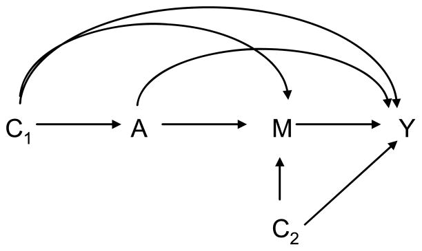
Causal Diagram for Mediation and Confounding

The variables in the graph are: exposure (A), mediator (M), outcome (Y), covariates (C=(C₁, C₂)), which include exposure-outcome confounders (C₁) and mediator-outcome confounders (C₂). All the comments below will still hold if C₁ affects C₂ or if C₂ affects C₁.

Consider the example of working activity of a drug addicted individual as the outcome of interest (Y). Let the treatment be methadone (A), and the potential mediator be the level of drug use (M). Under this scenario, the investigator may be interested in studying how the effect of the treatment A on the outcome Y is mediated by the level of drug use of an individual (M). In addressing this question of interest, the investigator must think carefully about and try to control for variables that may be exposure-outcome confounders (C₁) or mediator-outcome confounders (C₂). For example, there might be social and biological factors, such as income and hypertension status (C₁), that affect the decision of the level of treatment (A) and the working activity outcome (Y), or other factors, such as neighborhood of residence or alcohol consumption (C₂), which affect both the level of drug use (M) and the working activity outcome (Y).

In order for the effects to have a causal interpretation, control must be made for the confounding variables. In order to ensure identifiability of controlled direct effect, two assumptions are needed: namely those of (i) no unmeasured confounding of the treatment-outcome relationship and (ii) no unmeasured confounding of mediator-outcome relationship. The first of these assumptions would be automatically satisfied if treatment were randomized, but even with randomized treatment the second assumption might not be satisfied. If we refer to the example above, to control for (i) confounding of the treatment-outcome relationship the investigator must adjust for common causes of the treatment and the outcome e.g. information on income and hypertension status and any other treatment-outcome confounding variable (C₁) in the analysis. To control for (ii) mediator-outcome confounding the investigator must adjust for common causes of the mediator and the outcome e.g. alcohol consumption and neighborhood of residence or any other mediator-outcome confounding variable (C₂). In practice, both sets of covariates would simply be included in the overall set C for which adjustment is made; the investigator does not need to distinguish in this regression approach the treatment-outcome and the mediator-outcome confounding variables but the collection of covariates must include both sets for estimates to have a causal interpretation.

The assumptions we have described are for controlled direct effects; the identification of natural direct and indirect effects uses these two assumptions above along with two additional assumptions. In particular, for natural direct and indirect effects there must also be (iii) no unmeasured confounding of the treatment-mediator relationship. Control must be made for variables that cause both the level of treatment and the level of the mediator. In the context of our example, hypertension may be a factor which influences the use of treatment as well as the level of drug addiction, and it would need to be controlled for in the analysis. This third assumption, like the first, would also be satisfied automatically if the treatment were randomized. Finally, for the natural direct effect and indirect effects to be identified it also needs to be the case that (iv) there is no mediator-outcome confounder that is affected by the treatment (i.e. no arrow from A to C₂ in Figure 2).

It should be noted that assumptions (i), (ii), and (iii) also require an assumption of temporal ordering. This assumption of temporal ordering is implicitly or explicitly present in various approaches to mediation analysis (Cole and Maxwell, 2003). In particular, the assumption of no unmeasured confounding of the treatment-outcome relationship implicitly assumes that the treatment temporally precedes the outcome. The assumption of no unmeasured confounding of the mediator-outcome relationship implicitly assumes that mediator precedes temporally the outcome. Finally, the assumption of no unmeasured treatment-mediator confounding implicitly assumes that the exposure must precede the mediator. Formally the no unmeasured confounding assumptions require that associations reflect causal effects; if the temporal ordering assumptions were not satisfied then neither would the no unmeasured confounding assumptions since associations would not represent causal effects.

In summary, controlled direct effects require (i) no unmeasured treatment-outcome confounding and (ii) no unmeasured mediator-outcome confounding. Natural direct and indirect effects require these assumptions and also (iii) no unmeasured treatment-mediator confounding and (iv) no mediator-outcome confounder affected by treatment. It is important to note that randomizing the treatment is not enough to rule out confounding issues in mediation analysis. This is because randomization of the treatment rules out the problem of treatment-outcome and treatment-mediator confounding but does not guarantee that the assumption of no confounding of mediator-outcome relationship holds. This is because even if the treatment is randomized, the mediator generally will not be. This was pointed out by Judd and Kenny (1981), James et al. (1984), MacKinnon (2008), but unfortunately not mentioned in the popular paper by Baron and Kenny (1986). If there are confounders of the mediator-outcome relationship for which control has not been made, then direct and indirect effect estimates will not have a causal interpretation; they will be biased. This is true for the controlled direct effect and natural direct and indirect effects described above and also for the effects described by Baron and Kenny. Investigators should think more carefully about and collect data on and control for such mediator-outcome confounding variables when mediation analysis is of interest. If the investigator is aware that unmeasured confounding may be an issue in his or her study, sensitivity analyses (VanderWeele, 2010; Imai et al. 2010a) should be implemented.

Binary Outcome

We have thus far considered only the case in which both outcome and mediator are continuous. The results can be extended to cases in which one or both of the mediator and outcome variables are binary.

For example, when the outcome is binary and mediator is continuous the model for the mediator is represented by (1.1) and the outcome can be modeled via a logistic regression

$$\mathit{logit}\{P(Y=1\mid a,m,c)\}={\theta }_0+{\theta }_{1}a+{\theta }_{2}m+{\theta }_{3}am+{\theta }_4^{\prime }c$$ (0.4)

For this case, provided the outcome is relatively rare and assumptions (i)–(iv) hold, we can derive controlled direct effects, and natural direct and indirect effects on the odds ratio scale (VanderWeele and Vansteelandt, 2010a) as:

$$\begin{array}{l}log\{{OR}^{\mathit{CDE}}\}=({\theta }_1+{\theta }_{3}m)(a-a^{\ast })\\ log\{{OR}^{\mathit{NDE}}\}\cong \{{\theta }_1+{\theta }_3({\beta }_0+{\beta }_1{a}^{\ast }+{\beta }_2^{\prime }c+{\theta }_2{\sigma }^2)\}(a-a^{\ast })+0.5{\theta }_3^2{\sigma }^2(a^2-a^{\ast 2})\\ log\{{OR}^{\mathit{NIE}}\}\cong ({\theta }_2{\beta }_1+{\theta }_3{\beta }_{1}a)(a-a^{\ast })\end{array}$$

where σ₂ is the variance of the error term in the regression for the mediator, M, and where the approximations hold to the extent that the outcome Y is rare.

With these odds ratios, the total effect is equal to the product of the natural direct and indirect effects (rather than the sum).

When the outcome is not rare, the odds ratio does not approximate risk ratio anymore. Therefore, the causal effects previously defined will be biased if logistic regression is used to model the outcome. In this case the investigator can estimate the causal effect by running a generalized linear model regression with a binomial distribution and a log link and the causal effects will have a risk ratio interpretation and the formulas hold exactly.

When the outcome is rare then the direct and indirect effects can be estimated even in case-control designs. The formulas for the effects remain the same, however the mediator regression is run only for controls, to take into account the case-control design (VanderWeele and Vansteelandt, 2010). This approach works because with a rare outcome Y, the distribution of M among the controls will approximate the distribution in the population.

We also extend the previous results to the cases in which the mediator is a dichotomous variable. The identifiability assumptions do not change but now we would use a logistic model for the mediator:

$$\mathit{logit}\{P(M=1\mid a,c)\}={\beta }_0+{\beta }_{1}a+{\beta }_2^{\prime }c$$ (0.5)

Formulas for controlled direct effects and natural direct and indirect effects when the mediator is dichotomous are given in the appendix. Finally, in the online appendix we show that these formulas for causal effects for binary outcome, along with their standard errors, extend to count variables when modeled with a log link.

The total effect is computed as the sum of the natural direct effect and the natural indirect effect when the outcome is continuous and as the product of the natural direct and indirect effect odds ratios when the outcome is binary. Another measure that has been popular in mediation analysis is the proportion mediated. The proportion mediated can be defined as the ratio of the natural indirect effect to the total effect when the outcome is continuous; the proportion mediated on risk difference scale can also be calculated when the outcome is binary using a transformation of the odds ratios (VanderWeele and Vansteelandt, 2010a). Several authors have, however, issued cautions on its use. Kenny (1998) warns about the instability of such measure, especially when the association between the exposure and the outcome is weak. Consequently, we have not implemented this measure in the macro; however, investigators can certainly calculate these measures from the output that is provided.

Estimates described later in the paper of the direct and indirect effects of interest are obtained by plugging in the estimated coefficient values while the standard errors can be obtained using the delta method or by bootstrapping techniques. The reader can refer to the online supplement for derivations of the direct and indirect effects and delta method standard errors. The macro we provide will calculate these automatically.

Mediation analysis for models with non-linearities - a comparison of approaches

The counterfactual approach to mediation analysis displays all its power and flexibility when the causal relationships under study are complex and the investigator needs to depart from simple linear models and allow for non-linearities and interactions. In this section we describe some of the advantages of employing the counterfactual framework to causal mediation that we presented in the previous sections by comparing it to other popular methods to address mediation questions. In this comparison we will focus on the so-called product method, the difference method, and the MacArthur approach, and address also some developments with regard to “moderated mediation”. We first describe traditional statistical approaches and we then discuss what the counterfactual approach contributes over and above them and comment on the relation between the two.

Traditional approaches to mediation analysis

Modern approaches to mediation have been inspired by the pioneering work of the geneticist Sewall Wright (1920) who developed the path analysis method. Path analysis is now viewed as a special case of structural equation modeling (SEM). Structural equations methods allow for the estimation of direct and indirect effects by modeling covariance and correlation matrices. Most mediation analyses in psychological studies have been conducted using the structural equation modeling (SEM) approach (Baron and Kenny, 1986; Judd and Kenny, 1981; MacKinnon, 2008). Methods to improve estimation and inferential procedures for SEM-based mediation analyses have continued to develop (e.g. MacKinnon, 2008; Sobel, 1982). Structural equation models are often criticized for not adequately addressing issues of confounding/endogeneity in inferring causal relationships. However, if such issues of confounding are adequately addressed by including all relevant confounders (as described in detail above) in the structural equation model then the SEM approach can be a useful tool. The counterfactual approach has placed strong emphasis on identifiability assumptions and conceptual definitions of causal effects, and recently, a number of authors have been using the counterfactual framework to translate the SEM approach within the counterfactual framework¹ (e.g. Jo, 2008; Sobel, 2008; VanderWeele and Vansteelandt, 2009; Imai et al., 2010a; Pearl, 2011). Among traditional SEM methods, we describe the product method and the difference method. Assume a simple mediation model with no exposure-mediator interaction. The rationale behind the product method is that mediation depends on the extent to which the exposure A changes the mediator M, β₁ from equation (1.1), and the extent to which the mediator affects the outcome Y, θ₂ from equation (1.2). The product method estimator of the indirect effect is then simply θ₂β₁. Sobel (1982) proposed a test for a mediated effect from the product method estimator.

The difference method approach is implemented by fitting an outcome model with the mediator as in equation (2) and also an outcome model with no mediator:

$$E(\text{Y}\mid \text{a},\text{m},\text{c})={\theta }_0^{\ast }+{\theta }_1^{\ast }a+{{\theta }_4^{\ast }}^{\prime }c$$ (1.6)

The value of the mediated or indirect effect is then estimated by taking the difference in the coefficients from equations (1.6) and, ${\theta }_1^{\ast }-{\theta }_1$ this corresponds to the reduction in the independent variable effect on the dependent variable when adjustment is made for the mediator. The algebraic equivalence of the indirect effect using the product method, θ₂β₁, and the difference method, ${\theta }_1^{\ast }-{\theta }_1$ was shown by MacKinnon et al. (1995) for ordinary least squares in linear models with continuous outcomes and discussed also in Alwin and Hauser (1975). The product method and difference method diverge however when using a binary outcome and logistic regression (MacKinnon and Dwyer, 1993), a point to which we return below. When mediation models include an exposure-mediator interaction term in the outcome regression, this is a particular case or a variant of what is sometimes referred to as “moderated mediation” (James and Brett, 1984; Preacher et al., 2007). Moderated mediation considers the case in which a covariate moderates the mediated effect (cf. MacKinnon, 2007) i.e. when the mediated effect varies by the level of a covariate. Such moderated mediation by a covariate was also analyzed by Yzerbyt, Muller, and Judd (2004) and Muller, Yzerbyt and Judd (2008). When the treatment itself is the moderator for the mediator (as considered in Preacher et al. 2007), the effect of the mediator is allowed to vary by treatment status; or, conceived of another way, the effect of treatment is allowed to vary with (i.e. it interacts with) the mediator. In this setting, Preacher et al. (2007) derived an indirect effect estimator in the context of moderated mediation using the product method.

The MacArthur approach (Kraemer et al., 2008) gives criteria somewhat different than that of Baron and Kenny in assessing mediation and allows also for assessing exposure-mediator interactions. This approach to mediation analysis is based on the assumption that temporal antecedence and association are necessary (but not sufficient) for a causal relationship. The approach allows for non-linear relations among variables to qualify as mediation as long as there is a relationship between the exposure A, and the mediator M. In particular, it is proposed, first, that if there is no association between A and M, and if M precedes A, and if the A × M interaction is significant, then the variable M is to be considered as a moderator rather than a mediator. Second, for M to be a mediator for the effect of A on outcome Y, A should precede M and M should precede Y, the variables A and M should be correlated, and either the main effect of M on the outcome or the A × M interaction should be significant.

Comparison of traditional approaches with the counterfactual approach when there are interactions and non-linearities

One of the chief advantages of the counterfactual approach to mediation analysis is that it allows for the decomposition of a total effect into a direct effect and an indirect effect even when there are interactions and non-linearities. As noted above, some of the statistical approaches, such as that of Preacher et al. (2007) or Kraemer et al. (2008) allow one to assess mediation even when there is exposure-mediator interaction. In fact, the indirect effect of Preacher et al. (2007) for continuous outcome when there is an exposure-mediator interaction is equivalent to the one given here. However, neither Preacher et al. (2007) nor Kraemer et al. (2008) give a definition of a direct effect in the presence of exposure-mediator interaction such that the sum of the direct and indirect effects equals a total effect. The counterfactual approach provides a general approach to do effect decomposition irrespective of the statistical model and irrespective of possible interactions. The counterfactual approach coincides with the criteria for mediation of the MacArthur approach (Kraemer et al., 2008) but provides actual direct and indirect effect estimates that combine to a total effect and makes clear the no-unmeasured-confounding assumptions needed for a causal interpretation. The counterfactual approach also helps in understanding mediation with binary outcomes and binary mediators. As noted above, with a binary outcome and logistic regression, the product method and difference method give different results (MacKinnon and Dwyer, 1993). In fact, neither in general will be equal to an estimate of an indirect effect with a causal interpretation (VanderWeele and Vansteelandt, 2010). VanderWeele and Vansteelandt (2010) did, however, show that when there is no exposure-mediator interaction, the product method and difference method will be approximately equivalent when the outcome is rare; and both will then be approximately equal to the natural indirect effect when all the no confounding assumptions hold. The problem with dichotomous outcomes arises when the outcome is common and has to do with the fact that logistic regression uses the odds ratio, which is a measure that is “non-collapsible”. Viewed intuitively, the problem occurs because when the outcome is common, the odds ratio does not approximate the risk ratio, and the extent of this lack of approximation can vary with the other covariates in the models. With a common outcome, the odds ratios with the mediator in the model versus without the mediator in the model are thus not directly comparable, and so the difference method essentially breaks down. The risk ratio does not suffer this problem and it is for this reason that we propose using a log-linear model in this paper when the outcome is common. Moreover, this approach also allows us to define and estimate direct and indirect effects when the outcome is binary and an exposure-mediator interaction is present. We have moreover, using the counterfactual approach in this paper, derived analytic expressions for cases when the mediator itself is binary. The counterfactual approach provides a versatile framework to derive direct and indirect effects and to do effect decomposition even with binary variables and non-linear models.

As is perhaps now clear from this discussion, the traditional statistical approach and the counterfactual approach to mediation will in some settings coincide. For linear models and log-linear models, they will coincide when there is no exposure-mediator interaction; for logistic models, they will coincide when there is no exposure-mediator interaction and when the outcome is rare (VanderWeele and Vansteelandt, 2009, 2010). Thus, before an investigator proceeds with one of the traditional approaches (the product method or difference method) he or she should: (i) consider whether control has been made for exposure-outcome confounders, mediator-outcome confounders, and exposure-mediator confounders, (ii) check whether there is exposure-mediator interaction, and (iii) if the outcome is binary and logistic regression is used, check whether the outcome is rare. If the no-unmeasured-confounding conditions are satisfied, there is no interaction, and the outcome is rare if logistic regression is used, then proceeding with the traditional statistical approaches is fine. If there are exposure-mediator interactions then the approach described in this paper, or another counterfactual-based approach, should be used. If the outcome is common, a log-linear model can be used. If there are confounders of the exposure-outcome, mediator-outcome, or exposure-mediator relationship then, to the extent possible, these should be controlled for in the models; otherwise sensitivity analysis techniques (VanderWeele, 2010; Imai et al., 2010a) can be used.

As a final point of discussion, we note that even in the presence of interaction and non-linearities, the product method may be useful to test for mediation even if the estimates are not themselves interpretable as estimates of an indirect effect. In other words, to test for mediation we can test for whether the product of the coefficients is nonzero even if this product is not equal to a causal indirect effect measure. For example, with logistic model with common outcome, the product method estimates will not in general have a causal interpretation as a natural indirect effect. It is nonetheless the case that although the product-method estimator is not itself a measure of an indirect effect, the product method still gives a valid test for the presence of a mediated effect, provided that the identification assumptions hold and that the models are correctly specified (a formal proof of this is given in the e-Appendix of VanderWeele, 2011). The intuition is that even if the product of the coefficients is not equal to a causal indirect effect, if the product is non-zero then there must be an effect of the exposure on the mediator and an effect of the mediator on the outcome, and under the identification assumptions, this would also imply the presence of a natural indirect effect. Thus, the product-method approach can still be useful in testing for mediation even when there are interactions and non-linearities. For estimation and for decomposing a total effect into a direct and indirect effect (arguably the chief advantages of the counterfactual approach), rather than just testing, methods such as those described in this paper can be employed.

Description of the SAS macro

The present macro is designed to enable the investigator to easily implement mediation analysis in the presence of exposure-mediator interaction accounting for different types of outcomes (normal, dichotomous-logistic or dichotomous log-linear, poisson, negative binomial) and mediators of interest (normal or dichotomous with logit link). The logit link for dichotomous outcomes should only be used if the outcome is rare. If the outcome is not rare the log link can be used (though the outcome model may not always converge). In the case of using the log link the direct and indirect effects are on the risk ratio scale. In particular, these macros for SAS and SPSS provide estimates, and confidence intervals for the direct and indirect effects previously defined. The estimates assume the model assumptions are correct and the identifiability assumptions discussed in the previous section hold.

Basic SAS Macro

The macro has been developed using the 9.2 version of SAS software. In order to implement mediation analysis via the mediation macro in SAS the investigator first opens a new SAS session and inputs the data, which has to include the outcome, treatment and mediator variables as well as the covariates to be adjusted for in the model. Macro activation requires then the investigator to save the macro script and input information in the statement

% mediation(data= ,yvar= ,avar= ,mvar= ,cvar= ,a0= ,a1= ,m= ,nc= ,yreg= ,mreg= ,interaction=)
run;

First one inputs the name of the dataset (data=), then the name of the outcome variable (yvar=), the treatment variable (avar=), the mediator variable (mvar=), the other covariates, (cvar=). Categorical variables need to be coded as a series of dummy variables before being entered as covariates. The macro dumvar from MCHP SAS Macros, for example, can be used for this purpose. Then the investigator needs to specify the baseline level of the exposure a^* (a0=), the new exposure level a (a1=), the level of mediator m at which the controlled direct effect is to be estimated and the number of covariates to be used (nc=). When no covariates are entered, then the user still needs to write the commands cvar= and nc= even though both are left blank. The user must also specify which types of regression have to be implemented. In particular, linear, logistic, loglinear, poisson or negbin can be specified (yreg=). For the mediator either linear or logistic regressions are allowed (mreg=). Finally, the analyst needs to specify whether an exposure-mediator interaction is present (interaction= true or false).

The macro provides the following output: first the regression output for outcome and mediator models is provided. The output in the SAS macro is derived from the procedures of proc reg when the variable is continuous, proc logistic when the variable is binary. When the outcome is specified as poisson, negative binomial or log-linear the procedure proc genmod is employed. If the dataset contains missing data the macro implements a complete case only analysis. A table with direct and indirect effects together with total effects follows. The effects are reported for the mean level of the covariates C. The table contains standard errors, and confidence intervals for each effect.

Other options in the SAS Macro

The reduced output is the default option. The table will just display controlled direct effect, natural direct effect, natural indirect effect and total effect described above. When the option output=full is used, both conditional effects and effects evaluated at the mean covariate levels are shown. When the output=full option is chosen, the investigator must enter fixed values for the covariates C at which compute conditional effects. The macro statement is as follows:

%mediation(data= ,yvar= ,avar= ,mvar= ,cvar= ,a0= ,a1= ,m= ,nc= ,yreg= ,mreg= ,interaction=
,output= ,c=
)
run;

When output=full is added, then, in addition to the controlled direct effect, and the natural direct and indirect effects described above, other effects are also displayed. The natural direct and indirect effects we have been considering are sometimes called the “pure” natural direct effect and the “total” natural indirect effect (Robins and Greenland, 1992). We can also instead consider the “total” natural direct effect and the “pure” natural indirect effect. For binary exposure the total natural direct effect expresses how much the outcome would change on average if the exposure changed from level a^* =0 to level a=1, but the mediator for each individual was fixed at the natural level which would have taken at exposure level a=1. The pure natural indirect effect expresses how much the outcome would change on average if the exposure were controlled at level a^* =0 but the mediator were changed from the natural level it would take if a^* =0 to the level that would have taken at exposure level a=1. These effects are also reported if the user selects output=full. If there is no exposure-mediator interaction, the “pure” and “total” natural direct effects will coincide and the “pure” and “total” natural indirect effects will coincide. These different types of effects are essentially different ways of accounting for the exposure-mediator interaction (Robins, 2003; VanderWeele, 2012).

The investigator also has the option of implementing mediation analysis when data arise from a case-control design, provided the outcome in the population is rare. To do so the option casecontrol=true can be used. In this case the macro statement changes to:

%mediation(data= ,yvar= ,avar= ,mvar= ,cvar= ,a0= ,a1= ,m= ,nc= ,yreg= ,mreg= ,interaction=
,casecontrol=
)
run;

Finally, the investigator can choose whether to obtain standard errors and confidence intervals via the delta method or a bootstrapping technique. The default is the delta method. To use bootstrapping the option boot=true can be given. In this case the macro will compute 1,000 bootstrap samples from which causal effects are obtained along with their standard errors (s.e.) and percentile confidence intervals (p_95_CI_lower ,p_95_CI_upper). If the investigator wishes to use a higher number of bootstrap samples, instead of “true” he or she inputs the number of bootstrap samples desired (e.g. boot=5000 would estimate standard errors and confidence intervals using 5000 bootstrap samples). The use of bootstrap for standard errors is generally to be preferred if the sample size of the original sample is small as it will lead to more accurate inferences than the delta method (MacKinnon, 2008). However, these issues are less important if the original sample is large and if this is the case the use of delta method standard errors may be preferred because of computational efficiency. (For example, Ananth and VanderWeele (2011) conducted a mediation analysis using a sample of 26,000,000 individuals and bootstrapping would have been completely infeasible). When using the bootstrap the macro statement changes to:

%mediation(data= ,yvar= ,avar= ,mvar= ,cvar= ,a0= ,a1= ,m= ,nc= ,yreg= ,mreg= ,interaction=
,boot=
)
run;

As noted above, if the investigator wants to add a categorical variable as covariate, this must be recoded as a series of indicator variables. For example, if a covariate, named catvar, takes four levels (1,2,3,4) we could construct three “dummy” or “indicator” variables, named, for example, ivar2, ivar3, and ivar4, leaving the first value as the reference. The variable ivar2 would take the value 1 for all observations which had catvar=2, and 0 for all other observations. The variable ivar3 would take the value 1 for all observations that had catvar=3 and 0 for all other observations, etc. The macro dumvar mentioned previously requires the user to list the dataset (data=), the categorical variable (e.g. catvar) that needs to be transformed in the input (dvar=). The user needs also to input the prefix of the name of the dummy variables (e.g. ivar) that will be generated (prefix=) and the reference category (drop=). Categorical variables can be both character and numerical using dumvar. For example we can run the following:

dumvar data=dat dvar=“catvar” prefix=“ivar” drop=“ivar1”

Running this command will generate three indicator variables: “ivar2”, “ivar3”, “ivar4”. For more examples see: http://mchpappserv.cpe.umanitoba.ca/viewConcept.php?conceptID=1048.

Comparison with other macros

Before concluding the section we would like the reader to be aware that a rich set of alternative programs is also available to implement mediation analyses in certain settings. We believe that our macro provides unique features that may be useful to investigators. At the end of this section table 1 compares our macro to some of the existing and popular software tools. Preacher, Hayes et al. developed several macros for mediation mainly implementable in SAS, SPSS and Mplus (indirect, mediate, modmed, medcurve); Imai et al. also developed a macro in R (mediate). We also compare the macros to recent procedures that have been developed in Mplus (Muthén, 2012) in part based on the work we present in this paper. We compare the macros on the basis of certain features. We check whether they provide both direct and indirect effects and if they allow for nonlinearities such as interactions, and binary or count variables. We also consider whether they accommodate case-control designs and in which software packages they can be implemented.

Table 1.

Macro Comparison (^*Hayes and Preacher ^** Imai et al. ^***Valeri and VanderWeele ^† Muthen)

	mediation***	mediation**	modmed*	mediate*	Sobel*	Indirect*	medcurve*	M plus†
Causal Effects
direct effects	✓	✓	×	✓	×	✓	×	✓
indirect effects	✓	✓	✓	✓	✓	✓	✓	✓
Interaction
M-A	✓	✓	✓	×	×	×	×	✓
M-C	×	×	✓	×	×	×	×	✓
Type of variables
continuous M	✓	✓	✓	✓ (+ M & A)	✓	✓(+ M)	✓	✓
binary M	✓	✓	×	×	×	×	×	✓
continuous Y	✓	✓	✓	✓	✓	✓	✓	✓
binary Y	✓	✓	×	✓	✓	✓	×	✓
count Y	✓	✓	×	×	×	×	×	✓
ordinal Y	×	✓	×	×	×	×	×	✓
Additional covariate	✓	✓	✓	✓	×	✓	✓	✓
Design
Cross-Sectional	✓	✓	✓	✓	✓	✓	✓	✓
Cohort	✓	✓	✓	✓	✓	✓	✓	✓
Case-Control	✓	✓	×	×	✓	✓	×	×
Standard Errors
delta method	✓	×	×	×	×	×	×	✓
bootstrap	✓	✓	✓	✓	✓	✓	✓	✓
Software
SAS	✓	×	×	✓	✓	✓	✓	×
SPSS	✓	×	✓	✓	✓	✓	✓	×
R	×	✓	×	×	×	×	×	×
MPLUS	×	×	✓	×	×	×	×	✓

^† A number of the recent developments in Mplus were motivated by the results of the present paper

^** The Imai et al. (2009, 2010b) macros contain a sensitivity analysis option, Mplus is adding these features in keeping up with the literature and our macros will eventually have these features as well.

Our macro, in contrast with Preacher and Hayes’, (i) allows for effect decomposition into direct and indirect effects even in the presence of exposure-mediator interaction, (ii) allows for dichotomous mediators and count outcomes, (iii) allows for case-control designs, and (iv) gives estimates with a clear interpretation within the counterfactual framework. In contrast with that of Imai et al. (2010), our macro (i) provides direct and indirect effects on a ratio scale for dichotomous outcomes, (ii) allows for case-control sampling designs, (iii) is implemented in SAS and SPSS which are more commonly employed in the social sciences. Our macro provides similar features to Mplus which is in part because recent developments in Mplus (Muthén, 2012) were implemented following the results of our paper. Our macro, in contrast to Mplus, allows for case-control designs; Mplus, in contrast to our macro, allows for the flexibility to handle ordinal outcomes.

Description of the SPSS macro

The SPSS macro that we provide, which was developed under the version 19.0, performs exactly the same tasks described in the previous section for the SAS macro. However, we point out some small differences that the investigator has to take into account when running mediation analysis using SPSS software.

Before invoking the mediation macro the user has to open a new SPSS session and needs to specify the path in which he or she wants to save relevant estimates from the mediator and outcome regressions. This is simply done by running this command:

DEFINE !path()”C:\ “!ENDDEFINE.

In between the quotation marks the path is defined, here for example the path “C:\” has been entered. For SPSS users, macro activation requires that the macro script is then saved as a syntax file (the syntax file should be called from the session that has just been opened) and information is input in the following statement:

mediation data= / yvar= /avar= /mvar= /cvar= /NC= /a0= /a1= /m= /yreg= /mreg= /interaction=
[/casecontrol= /Output= /c=]

First one inputs the name of the dataset (including the path, e.g. data=“C:\mydata.sav”), then the name of the outcome variable (yvar=), the treatment variable (avar=), the mediator variable (mvar=), and the other covariates (cvar=). Categorical variables need to be coded as a series of dummy variables before being entered as covariates. The macro dummit can be used for this purpose. Then the investigator needs to specify the baseline level of the exposure a^* (a0=), the new exposure level a (a1=), the level of mediator m at which the controlled direct effect is to be estimated and the number of covariates to be used (nc=). When no covariates are entered, then the user still needs to write the command cvar= and needs to specify that nc=0. The user must also specify which types of regression have to be implemented. In particular, LINEAR, LOGISTIC, LOGLINEAR, POISSON or NEGBIN can be specified in the option yreg. Logistic links for yreg can be used for rare dichotomous outcomes; otherwise for dichotomous outcomes that are not rare, log links should be used for the outcome regression and the effects are then given on the risk ratio scale. For the option mreg either LINEAR or LOGISTIC regressions are allowed. If the dataset contains missing data the macro implements a complete case only analysis.

Finally, the analyst needs to specify whether an exposure-mediator interaction is present (TRUE or FALSE). As optional inputs, the investigator can use the option casecontrol=TRUE, when the data arise from a case-control study and the outcome is rare. More complete output (described in the previous section) can be obtained using the option Output=FULL and entering the values for the covariates at which to compute causal effects conditional on those covariate values (c=). In order to enter the covariate values the investigator needs to create a separate dataset that contains those values. For example, if two covariates C are present in the model and the value at which the investigator wants to fix the first is 4 and the value at which the investigator wants to fix the second is 10, at the beginning of the script the following commands need to be run:

Matrix.
compute c=make(1,2,0).
compute c(1,1)=4.
compute c(1,2)=10.
SAVE {c(1,:)} /OUTFILE=“C:\c.sav”.
end matrix.

After having created dataset for the covariate values, the user can specify the option Output=FULL/c=“C:\c.sav” to obtain the more complete output.

If the investigator wishes to obtain bootstrap standard errors, he or she can use the option boot=true followed by the number of observations in the dataset (nobs=) to compute causal effects and standard errors with 1,000 bootstrap replications (or “boot=n”, where n is the desired number of bootstrap samples). Otherwise delta method standard errors is the default option.

As we mentioned in the previous section, if the investigator needs to add a categorical variable as covariate, a series of indicator variables needs to be generated. The SPSS macro dummit works very similarly to the SAS macro. In particular the investigator needs to call the macro followed by three parentheses. In the first parenthesis the number of levels is entered, in the second parenthesis the name of the variable needs to be specified. Finally, in the third parenthesis, the prefix for the new variables is entered. For example if the variable we need to recode is “smoking” which takes levels “never”, “past”, “current”. Then we can run the following macro:

dummit (3) (smoking) (smoke)

This macro would generate the following variables: “smokedum2”, “smokedum3”. The category “never” is automatically taken as a reference. More examples can be found following the link: http://www.glennlthompson.com/?p=92.

Example

We present in this section an example of using the mediation macro. We implement the analyses on a modified version of the fictitious dataset used by Preacher and Hayes (2004) to explain their Sobel macro. The interest lies in the effects of a new cognitive therapy on life satisfaction after retirement. Residents of a retirement home diagnosed as clinically depressed are randomly assigned to receive 10 sessions of a new cognitive therapy (A=1) or 10 sessions of an alternative therapeutic method (A=0). After Session 8, the positivity of the evaluation the residents make for a recent failure experience is assessed (M). Finally, at the end of Session 10, the residents are given a questionnaire to measure life satisfaction (Y). The question is whether the cognitive therapy’s effect on life satisfaction is mediated by the positivity of their attributions of negative experiences.

The new dataset that we employ differs with respect to Preacher and Hayes’ one only in the way in which the outcome is simulated. In particular, the exposure and mediator variables are the same but now the outcome is simulated as a normally distributed variable with mean equal to the linear regression estimated with the original data (the coefficients given in the outcome regression in Preacher and Hayes, 2004) plus a new term, the exposure-mediator interaction term, with coefficient equal to θ₃=0.5 indicating a weak positive interaction, and standard deviation equal to the standard error of the residuals obtained from the outcome regression using Preacher and Hayes data (http://www.afhayes.com/spss-sas-and-mplus-macros-and-code.html).

We first consider the case in which the interaction between the therapy and the attributions of negative experiences is omitted by the investigator.

After having saved the dataset and inserted macro script we run the following command:

%mediation(data=dat ,yvar=satis ,avar=therapy ,mvar=attrib ,cvar= ,a0=0 ,a1=1 ,m=0, nc=
,yreg=linear ,mreg=linear ,interaction=false
)
run;

The first output provided is the results of the outcome and mediator regressions:

Dependent Variable: satis
Parameter Standard
Variable	DF	Estimate	s.e.	t -value	Pr > |t|
Intercept	1	−0.71479	0.20449	−3.50	0.0017
therapy	1	0.66788	0.30147	2.22	0.0354
attrib	1	0.67186	0.16923	3.97	0.0005

Dependent Variable: attrib
Parameter Standard
Variable	DF	Estimate	s.e.	t -value	Pr > |t|
Intercept	1	−0.35357	0.21837	−1.62	0.1166
therapy	1	0.81857	0.29902	2.74	0.0106

Then the direct effects and indirect effects follow. We give the reduced output, which provides estimates for the controlled direct effect, the natural indirect effect, and the total effect:

Obs	Effect	Estimate	s.e.	p_value	CI_95lower	CI_95upper
1	cde=nde	0.66788	0.30147	0.026733	0.07700	1.25877
2	nie	0.54997	0.24403	0.024215	0.07167	1.02827
3	total effect	1.21785	0.33475	0.000275	0.56174	1.87396

We then run the mediation macro with the correctly specified outcome regression model that includes the exposure-mediator interaction term. We type the following command:

%mediation(data=dat ,yvar=satis ,avar=therapy ,mvar=attrib ,cvar= ,a0=0 ,a1=1 ,m=0 ,nc=
,yreg=linear ,mreg=linear, interaction=true
)
run;

The output from the outcome regression is the following (the mediator regression will be the same):

Dependent Variable: satis
Parameter Standard
Variable	DF	Estimate	s.e.	t -value	Pr > |t|
Intercept	1	−0.84424	0.1964	−4.30	0.0002
therapy	1	0.62132	0.27901	2.23	0.0348
attrib	1	0.30575	0.21913	1.40	0.1747
int	1	0.74464	0.31251	2.38	0.0248

We obtain the following estimates for the effects:

Obs	Effect	Estimate	s.e.	p_value	CI_95lower	CI_95upper
1	cde	0.62132	0.27901	0.02596	0.07446	1.16818
2	nde	0.35804	0.34759	0.30298	−0.32323	1.03931
3	nie	0.85981	0.28782	0.00281	0.29568	1.42395
4	total effect	1.21785	0.33407	0.00027	0.56307	1.87263

We can see how the estimate of the indirect effect is downward biased and is less significant if the interaction term is omitted. Moreover, when the interaction term is correctly added in the model, controlled direct effects and natural direct effects differ.

Discussion

With the present work we have provided several contributions that will likely be important for research in psychology and in the social and biomedical sciences. First, by using a counterfactual approach for the definition of the causal effects of interest, along with their identifiability conditions, we give the reader some intuitive rules allowing for causal interpretation in mediation analysis. Issues of identification and causal interpretation have often been neglected when using the Baron and Kenny approach and other traditional approaches; the overview here will hopefully guide researchers in thinking about these questions. Second, we have described how progress in mediation analysis can be made in the case in which exposure-mediator interaction is present and we have derived new formulas in the appendix for settings with a binary mediator allowing for exposure-mediator interactions. We have also extended this approach to count outcomes. Third, the investigator who wishes to pursue mediation analysis using regression models will find useful resources in the SAS and SPSS macro that we developed. These macros target the implementation of mediation analysis allowing for the presence of exposure-mediator interaction. The macro was created by applying and extending the work on identification and estimation of direct and indirect causal effects of VanderWeele and Vansteelandt (2009, 2010). We provided a table that summarizes the features of the most popular existing macros for mediation. The current macro also allows for binary and count data as outcomes and provides valid estimation under case-control designs provided the outcome is rare.

Mediation analysis from a counterfactual perspective with exposure-mediator interaction can also be performed in R and STATA using the macro provided by Imai et al. (2010a, 2010b). Their approach to mediation analysis relies on Monte Carlo methods. However, the connections to product method and other popular methods in mediation analysis are clearer with the regression-based approach we have presented in that we have provided analytic formulae for the direct and indirect effects and these formulae coincide with the product method when there are no interactions. The approach of Imai et al. (2010a, 2010b) has the advantage of not needing separate formulas for each combination of the mediator and outcome models (since the calculations are done by simulation). It has the disadvantage of being much more computationally intensive which may prohibit use in large datasets.

The reader should note that if interactions between exposure or mediator and additional covariates (C) are present, these might need to be included in order to have a correctly specified model. However, the identifiability conditions that we described above under the counterfactual framework are applicable also to these more complex models. An investigator can still pursue mediation analysis with these different models, but new formulas for the direct and indirect effects defined above would have to be derived. The derivations in the online appendix provide a template that could be used to derive these new formulas for the direct and indirect effects and their standard errors in other types of models that may include interactions between covariates and treatment or mediator or quadratic terms.

Finally we emphasize that the investigator needs to take particular care in controlling for mediator-outcome confounding. The estimates from the product method or difference method or our approach will be biased if control is not made for these variables. Mediator-outcome confounding can be present even if the exposure is randomized (since the mediator is not randomized). Unfortunately, this point was not made in the popular Baron and Kenny (1986) paper, though it was made by Judd and Kenny (1981) five years earlier and it has now been emphasized and clarified in the causal inference literature and is being emphasized again in psychology. Psychologists, social scientists, and biomedical researchers need to take this assumption seriously if they hope to obtain valid conclusions about direct and indirect effects. If the investigator thinks that unmeasured confounding may be present, sensitivity analysis should be used (VanderWeele, 2010b; Imai et al. 2010a). We hope to automate sensitivity analysis in the macro in future work.

The authors thank David MacKinnon for helpful comments. The research was supported by NIH grants ES017876 and HD060696.

Appendix

We let Y_a and M_a denote respectively the values of the outcome and mediator that would have been observed had the exposure A been set to level a. We let Y_am denote the value of the outcome that would have been observed had the exposure A, and mediator, M, been set to levels a, and m, respectively. The average controlled direct effect comparing exposure level a to a^* and fixing the mediator to level m is defined by CDE_a,a^* (m) = E[Y_am − Y_a^*m]. The average natural direct effect is then defined by NDE_a,a^* (a^*) = E[Y_aMa^* − Y_a^*Ma^*]. The average natural indirect effect can be defined as NIE_a,a^* (a^*) = E[Y_aMa − Y_aMa^*], which compares the effect of the mediator at levels M_a and M_a^* on the outcome when exposure A is set to a. Controlled direct effects and natural direct and indirect effects within strata of C=c are then defined by: CDE_a,a^*|c (m) = E[Y_am − Y_a^*m|c], NDE_a,a^*|c (a^*) = E[Y_aMa^* − Y_a^*Ma^*|c], and NIE_a,a^*|c (a^*) = E[Y_aMa − Y_aMa^*|c], respectively.

For a dichotomous outcome the total effect on the odds ratio scale conditional on C=c is given by ${OR}_{a,a^{\ast }\mid c}^{TE}=\frac{P(Y_a=1\mid c)/\{1-P(Y_a=1\mid c)\}}{P(Y_{a^{\ast }}=1\mid c)/\{1-P(Y_{a^{\ast }}=1\mid c)\}}$. The controlled direct effect on the odds ratio scale is given by ${OR}_{a,a^{\ast }\mid c}^{\mathit{CDE}}(m)=\frac{P(Y_{am}=1\mid c)/\{1-P(Y_{am}=1\mid c)\}}{P(Y_{a^{\ast }m}=1\mid c)/\{1-P(Y_{a^{\ast }m}=1\mid c)\}}.$. The natural direct effect on the odds ratio scale conditional on C=c is given by ${OR}_{a,a^{\ast }\mid c}^{\mathit{NDE}}(a^{\ast })=\frac{P(Y_{{aM}_{a^{\ast }}}=1\mid c)/\{1-P(Y_{{aM}_{a^{\ast }}}=1\mid c)\}}{P(Y_{a^{\ast }{M}_{a^{\ast }}}=1\mid c)/\{1-P(Y_{a^{\ast }{M}_{a^{\ast }}}=1\mid c)\}}$. The natural indirect effect on the odds ratio scale conditional on C=c is given by ${OR}_{a,a^{\ast }\mid c}^{\mathit{NIE}}(a)=\frac{P(Y_{{aM}_a}=1\mid c)/\{1-P(Y_{{aM}_a}=1\mid c)\}}{P(Y_{{aM}_{a^{\ast }}}=1\mid c)/\{1-P(Y_{{aM}_{a^{\ast }}}=1\mid c)\}}$.

As discussed in the text, identification assumptions (i)–(iv) will suffice to identify these direct and indirect effects. If we let X⊥ Y | Z denote that X is independent of Y conditional on Z then these four identification assumptions can be expressed formally in terms of counterfactual independence as (i) Y_am ⊥ A | C , (ii) Y_am ⊥ M |{A,C} , (iii) M_a ⊥ A | C , and (iv) Y_am ⊥ M_a^* | C.Assumptions (i) and (ii) suffice to identify controlled direct effects; assumptions (i)–(iv) suffice to identify natural direct and indirect effects (Pearl, 2001; VanderWeele and Vansteelandt, 2009). The intuitive interpretation of these assumptions as described in the text follows from the theory of causal diagrams interpreted as non-parametric structural equations (Pearl, 2001). Alternative identification assumptions have also been proposed (Imai 2010a; Hafeman and VanderWeele, 2011). However, it has been shown that the intuitive graphical interpretations of these alternative assumptions are in fact equivalent (Shpitser and VanderWeele, 2011). Technical examples can be constructed where one set of identification assumptions holds and another does not (see also Robins and Richardson, 2010), but on a causal diagram corresponding to a set of non-parametric structural equations, whenever one set of the assumptions among those in VanderWeele and Vansteelandt (2009), Imai (2010a), and Hafeman and VanderWeele (2011) holds, the others will also.

Continuous Outcome and Continuous Mediator

Suppose that both the mediator and the outcome are continuous and that the following models fit the observed data:

$$E[M\mid a,c]={\beta }_0+{\beta }_{1}a+{\beta }_2^{\prime }c$$

$$E[Y\mid a,m,c]={\theta }_0+{\theta }_{1}a+{\theta }_{2}m+{\theta }_{3}am+{\theta }_4^{\prime }c$$

If the covariates C satisfied the no-unmeasured confounding assumptions (i)–(iv) above, then the average controlled effect and the average natural direct and indirect effects would be given by (VanderWeele and Vansteelandt, 2009):

$$\begin{array}{l}\mathit{CDE}=({\theta }_1+{\theta }_{3}m)(a-a^{\ast })\\ \mathit{NDE}=\{{\theta }_1+{\theta }_3({\beta }_0+{\beta }_1{a}^{\ast }+{\beta }_2^{\prime }c)\}(a-a^{\ast })\\ \mathit{NIE}=({\theta }_2{\beta }_1+{\theta }_3{\beta }_{1}a)(a-a^{\ast })\end{array}$$

Continuous Outcome and Binary Mediator

Suppose that the mediator is binary and the outcome is continuous and that the following models fit the observed data:

$$\begin{array}{l}E[Y\mid a,m,c]={\theta }_0+{\theta }_{1}a+{\theta }_{2}m+{\theta }_{3}am+{\theta }_4^{\prime }c\\ \mathit{logit}\{P(M=1\mid a,c)\}={\beta }_0+{\beta }_{1}a+{\beta }_2^{\prime }c\end{array}$$

If the covariates C satisfied the no-unmeasured confounding assumptions (i)–(iv) above, then the average controlled effect and the average natural direct and indirect effects would be given by:

$$\begin{array}{l}\mathit{CDE}=({\theta }_1+{\theta }_{3}m)(a-a^{\ast })\\ \mathit{NDE}={\theta }_1(a-a^{\ast })+\{{\theta }_3(a-a^{\ast })\}\frac{exp({\beta }_0+{\beta }_1{a}^{\ast }+{\beta }_2^{\prime }c)}{1+exp({\beta }_0+{\beta }_1{a}^{\ast }+{\beta }_2^{\prime }c)}\\ \mathit{NIE}=({\theta }_2+{\theta }_{3}a)\{\frac{exp({\beta }_0+{\beta }_{1}a+{\beta }_2^{\prime }c)}{1+exp({\beta }_0+{\beta }_{1}a+{\beta }_2^{\prime }c)}-\frac{exp({\beta }_0+{\beta }_1{a}^{\ast }+{\beta }_2^{\prime }c)}{1+exp({\beta }_0+{\beta }_1{a}^{\ast }+{\beta }_2^{\prime }c)}\}\end{array}$$

Binary Outcome and Continuous Mediator

Suppose that the mediator is continuous and the outcome is binary and rare and that the following models fit the observed data:

$$\begin{array}{l}\mathit{logit}\{P(Y=1\mid a,m,c)\}={\theta }_0+{\theta }_{1}a+{\theta }_{2}m+{\theta }_{3}am+{\theta }_4^{\prime }c\\ E[M\mid a,c]={\beta }_0+{\beta }_{1}a+{\beta }_2^{\prime }c\end{array}$$

If the covariates C satisfied the no-unmeasured confounding assumptions (i)–(iv) above, then the average controlled effect and the average natural direct and indirect effects would be given approximately by:

$$\begin{array}{l}log\{{OR}^{\mathit{CDE}}\}=({\theta }_1+{\theta }_{3}m)(a-a^{\ast })\\ log\{{OR}^{\mathit{NDE}}\}\cong \{{\theta }_1+{\theta }_3({\beta }_0+{\beta }_1{a}^{\ast }+{\beta }_2^{\prime }c+{\theta }_2{\sigma }^2)\}(a-a^{\ast })+0.5{\theta }_3^2{\sigma }^2(a^2-a^{\ast 2})\\ log\{{OR}^{\mathit{NIE}}\}\cong ({\theta }_2{\beta }_1+{\theta }_3{\beta }_{1}a)(a-a^{\ast })\end{array}$$

These expressions apply also if the outcome is not rare and log-linear rather than logistic models are fit to the data; the expressions are then for direct and indirect effect risk ratios rather than odds ratios.

Binary Outcome and Binary Mediator

Suppose that both the mediator and the outcome are binary and that the following models fit the observed data:

$$\begin{array}{l}\mathit{logit}\{P(Y=1\mid a,m,c)\}={\theta }_0+{\theta }_{1}a+{\theta }_{2}m+{\theta }_{3}am+{\theta }_4^{\prime }c\\ \mathit{logit}\{P(M=1\mid a,c)\}={\beta }_0+{\beta }_{1}a+{\beta }_2^{\prime }c\end{array}$$

If the covariates C satisfied the no-unmeasured confounding assumptions (i)–(iv) above, then the average controlled effect and the average natural direct and indirect effects would be given by:

$$\begin{array}{l}{OR}^{\mathit{CDE}}=exp\{({\theta }_1+{\theta }_{3}m)(a-a^{\ast })\}\\ {OR}^{\mathit{NDE}}\cong \frac{exp({\theta }_{1}a)\{1+exp({\theta }_2+{\theta }_{3}a+{\beta }_0+{\beta }_1{a}^{\ast }+{\beta }_2^{\prime }c)\}}{exp({\theta }_1{a}^{\ast })\{1+exp({\theta }_2+{\theta }_3{a}^{\ast }+{\beta }_0+{\beta }_1{a}^{\ast }+{\beta }_2^{\prime }c)\}}\\ {OR}^{\mathit{NIE}}\cong \frac{\{1+exp({\beta }_0+{\beta }_1{a}^{\ast }+{\beta }_2^{\prime }c)\}\{1+exp({\theta }_2+{\theta }_{3}a+{\beta }_0+{\beta }_{1}a+{\beta }_2^{\prime }c)\}}{\{1+exp({\beta }_0+{\beta }_{1}a+{\beta }_2^{\prime }c)\}\{1+exp({\theta }_2+{\theta }_{3}a+{\beta }_0+{\beta }_1{a}^{\ast }+{\beta }_2^{\prime }c)\}}\end{array}$$

These expressions apply also if the outcome is not rare and log-linear rather than logistic models are fit to the data; the expressions are then for direct and indirect effect risk ratios rather than odds ratios. As discussed in the online supplement, the expressions for binary outcomes also apply to count outcomes using models with log links. Derivations and standard errors are also given in the online supplement.

References

- Alwin DF, Hauser RM. The decomposition of effects in path analysis. American Sociological Review. 1975;40:37–47. [Google Scholar]
- Ananth CV, VanderWeele TJ. Placental abruption and perinatal mortality with preterm delivery as a mediator: disentangling direct and indirect effects. American Journal of Epidemiology. 2011;174:99–108. doi: 10.1093/aje/kwr045. [DOI] [PMC free article] [PubMed] [Google Scholar]
- Baron RM, Kenny DA. The moderator-mediator variable distinction in social psychological research: Conceptual, strategic, and statistical considerations. Journal of Personality and Social Psychology. 1986;51:1173–1182. doi: 10.1037//0022-3514.51.6.1173. [DOI] [PubMed] [Google Scholar]
- Cole DA, Maxwell SE. Testing mediational models with longitudinal data: Questions and tips in the use of structural equation modeling. Journal of Abnormal Psychology. 2003;112:558–577. doi: 10.1037/0021-843X.112.4.558. [DOI] [PubMed] [Google Scholar]
- Hafeman DM, VanderWeele TJ. Alternative assumptions for the identification of direct and indirect effects. Epidemiology. 2011;22:753–764. doi: 10.1097/EDE.0b013e3181c311b2. [DOI] [PubMed] [Google Scholar]
- Huang B, Sivaganesan S, Succop P, Goodman E. Statistical assessment of mediational effects for logistic mediational models. Statistics in Medicine. 2004;23:2713–2728. doi: 10.1002/sim.1847. [DOI] [PubMed] [Google Scholar]
- Hyman HH. Survey design and analysis: Principles, cases and procedures. Glencoe, IL: Free Press; 1955. [Google Scholar]
- Imai K, Keele L, Yamamoto T. Identification, inference, and sensitivity analysis for causal mediation effects. Statistical Science. 2009;25:5171. doi: 10.1214/10-STS321.. [DOI] [Google Scholar]
- Imai K, Keele L, Tingley D. A General Approach to Causal Mediation Analysis. Psychological Methods. 2010a;15(4):309–334. doi: 10.1037/a0020761. [DOI] [PubMed] [Google Scholar]
- Imai K, Keele L, Tingley D, Yamamoto T. Causal Mediation Analysis Using R. In: Vinod HD, editor. Advances in Social Science Research Using R. New York: Springer; 2010b. pp. 129–154. [Google Scholar]
- James LR, Brett JM. Mediators, moderators, and tests for mediation. Journal of Applied Psychology. 1984;69:307321. [Google Scholar]
- Jo B. Causal inference in randomized experiments with mediational processes. Psychological Methods. 2008;13:314–336. doi: 10.1037/a0014207. [DOI] [PMC free article] [PubMed] [Google Scholar]
- Joffe M, Small D, Hsu C-Y. Defining and estimating intervention effects for groups that will develop an auxiliary outcome. Statistical Science. 2007;22:74–97. doi: 10.1214/088342306000000655.. [DOI] [Google Scholar]
- Judd CM, Kenny DA. Process analysis: estimating mediation in treatment evaluations. Evaluation Review. 1981;5:602–619. [Google Scholar]
- Kraemer HC, Kiernan M, Essex M, Kupfer DJ. How and why the criteria defining moderators and mediators differ between the Baron & Kenny and MacArthur Approaches. Health Psychology. 2008;27(2 Suppl):S101–S108. doi: 10.1037/0278-6133.27.2(Suppl.).S101. [DOI] [PMC free article] [PubMed] [Google Scholar]
- MacKinnon DP, Dwyer JH. Estimating mediated effects in prevention studies. Evaluation Review. 1993;17:144–158. [Google Scholar]
- MacKinnon DP. Introduction to Statistical Mediation Analysis. New York: Erlbaum; 2008. [Google Scholar]
- Muller D, Yzerbyt V, Judd CM. Adjusting for a mediator in models with two crossed treatment variables. Organizational Research Methods. 2008;11:224–240. [Google Scholar]
- Muthén B. Applications of causally defined direct and indirect effects in mediation analysis using SEM in Mplus. 2012 Submitted for publication. [Google Scholar]
- Pearl J. Proceedings of the Seventeenth Conference on Uncertainty in Artificial Intelligence. San Francisco, CA: Morgan Kaufmann; 2001. Direct and Indirect Effects; pp. 411–420. é. [Google Scholar]
- Preacher KJ, Hayes AF. SPSS and SAS procedures for estimating indirect effects in simple mediation models. Behavior Research Methods, Instruments, and Computers. 2004;36:717–731. doi: 10.3758/bf03206553. [DOI] [PubMed] [Google Scholar]
- Preacher KJ, Rucker DD, Hayes AF. Addressing moderated mediation hypotheses: Theory, methods, and prescriptions. Multivariate Behavioral Research. 2007;42(1):185–227. doi: 10.1080/00273170701341316. [DOI] [PubMed] [Google Scholar]
- Robins JM. Semantics of causal DAG models and the identification of direct and indirect effects. In: Green P, Hjort NL, Richardson S, editors. Highly Structured Stochastic Systems. Oxford University Press; New York: 2003. pp. 70–81. [Google Scholar]
- Robins JM, Greenland S. Identifiability and exchangeability for direct and indirect effects. Epidemiology. 1992;3:143–155. doi: 10.1097/00001648-199203000-00013. [DOI] [PubMed] [Google Scholar]
- Robins JM, Richardson TS. Alternative graphical causal models and the identification of direct effects. In: Shrout P, editor. Causality and Psychopathology: Finding the Determinants of Disorders and Their Cures. Oxford University Press; 2010. [Google Scholar]
- Shpitser I, VanderWeele TJ. A complete graphical criterion for the adjustment formula in mediation analysis. International Journal of Biostatistics, 7, Article. 2011;16:1–24. doi: 10.2202/1557-4679.1297. [DOI] [PMC free article] [PubMed] [Google Scholar]
- Sobel ME. Asymptotic confidence intervals for indirect effects in structural equations models. In: Leinhart S, editor. Sociological methodology. San Francisco: Jossey-Bass; 1982. pp. 290–312. [Google Scholar]
- Sobel ME. Identification of causal parameters in randomized studies with mediating variables. Journal of Educational and Behavioral Statistics. 2008;33:230–251. [Google Scholar]
- VanderWeele TJ, Vansteelandt S. Conceptual issues concerning mediation, interventions and composition. Statistics and Its Interface. 2009;2(4):457–468. [Google Scholar]
- VanderWeele TJ, Vansteelandt S. Odds Ratios for Mediation Analysis for a Dichotomous Outcome. Am J Epidemiol. 2010;172(12):1339–1348. doi: 10.1093/aje/kwq332. [DOI] [PMC free article] [PubMed] [Google Scholar]
- VanderWeele TJ. Bias formulas for sensitivity analysis for direct and indirect effects. Epidemiology. 2010;21:540–551. doi: 10.1097/EDE.0b013e3181df191c. [DOI] [PMC free article] [PubMed] [Google Scholar]
- VanderWeele T. Causal Mediation Analysis with Survival Data. Epidemiology. 2011;22:575581. doi: 10.1097/EDE.0b013e31821db37e. [DOI] [PMC free article] [PubMed] [Google Scholar]
- VanderWeele TJ. A three-way decomposition of a total effect into direct, indirect, and interactive effects. Epidemiology. 2012 doi: 10.1097/EDE.0b013e318281a64e. in press. [DOI] [PMC free article] [PubMed] [Google Scholar]
- Yzerbyt V, Muller D, Judd CM. Adjusting researchers’ approach to adjustment: On the use of covariates when testing interactions. Journal of Experimental Social Psychology. 2004;40:424–431. [Google Scholar]
Associated Data
This section collects any data citations, data availability statements, or supplementary materials included in this article.