A comparative analysis of biclustering algorithms for gene expression data

Abstract

The need to analyze high-dimension biological data is driving the development of new data mining methods. Biclustering algorithms have been successfully applied to gene expression data to discover local patterns, in which a subset of genes exhibit similar expression levels over a subset of conditions. However, it is not clear which algorithms are best suited for this task. Many algorithms have been published in the past decade, most of which have been compared only to a small number of algorithms. Surveys and comparisons exist in the literature, but because of the large number and variety of biclustering algorithms, they are quickly outdated. In this article we partially address this problem of evaluating the strengths and weaknesses of existing biclustering methods. We used the BiBench package to compare 12 algorithms, many of which were recently published or have not been extensively studied. The algorithms were tested on a suite of synthetic data sets to measure their performance on data with varying conditions, such as different bicluster models, varying noise, varying numbers of biclusters and overlapping biclusters. The algorithms were also tested on eight large gene expression data sets obtained from the Gene Expression Omnibus. Gene Ontology enrichment analysis was performed on the resulting biclusters, and the best enrichment terms are reported. Our analyses show that the biclustering method and its parameters should be selected based on the desired model, whether that model allows overlapping biclusters, and its robustness to noise. In addition, we observe that the biclustering algorithms capable of finding more than one model are more successful at capturing biologically relevant clusters.

INTRODUCTION

Microarray technology enables the collection of vast amounts of gene expression data from biological systems. A single microarray chip can collect expression levels from thousands of genes, and these data are often collected from multiple tissues, in multiple patients, with different medical conditions, at different times, and in multiple trials. For instance, the Gene Expression Omnibus (GEO), a public database of gene expression data, currently contains 659 203 samples on 9528 different microarray platforms [1]. These large quantities of high-dimensional data sets are driving the search for better algorithms and more sophisticated analysis methods.

Clustering has been one successful approach to exploring this data. Clustering algorithms seek to partition objects into clusters to maximize within-cluster similarity, or minimize between-cluster similarity, based on a similarity measure. Given a two-dimensional gene expression matrix M with m rows and n columns, in which the n columns contain samples, and each sample consists of gene expression levels for m probes, a cluster analysis could either cluster rows or columns. It is also possible to seperately cluster rows and columns, but a more fine-grained approach, biclustering, allows simultaneous clustering of both rows and columns in the data matrix. This method is useful to capture the genes that are correlated only in a subset of samples. Such clusters are biologically interesting since they not only allow us to capture the correlated genes, but also enable the identification of genes that do not behave similar in all conditions. Hence, biclustering is more likely to yield the discovery of biological clusters that a clustering algorithm might fail to recover.

The concept of biclustering was first introduced in [2], and applied to gene expression data by Cheng and Church [3]. Many other such algorithms have been published since [4–7]. Moreover, there have been some other algorithms proposed to address different biclustering problems [8], such as time series gene expression data. Biclustering became a popular tool for discovering local patterns on gene expression data since many biological activities are common to a subset of genes and they are co-regulated under certain conditions.

Most biclustering problems are exponential in the rows and columns of the dataset (m and n), so algorithms must depend on heuristics, making their performance suboptimal. Since the ground truth of real biological datasets is unknown, it is difficult to verify a biclustering's biological relevance. Therefore, there exists no consensus of which biclustering approaches are most promising.

In this article, we further attempt at comparing biclustering algorithms by making the following improvements. First, we compare 12 biclustering algorithms, many of which have only recently been published and not extensively studied. Second, rather than using default parameters, each algorithm's parameters were tuned specifically for each dataset. Third, although each method is proposed to optimize a different model, earlier comparative analysis papers generated synthetic datasets from only one model, resulting an unfair comparison. We use six different bicluster models to find the best for each algorithm. In addition, previous papers used only one or two real datasets, often obtained from Saccharomyces cerevisiae or Escherichia coli. Most did not perform multiple test correction when performing Gene Ontology enrichment analysis. We used eight datasets from GEO, all but one of which have over 12 000 genes, and biclusters were considered enriched only after multiple test correction.

RELATED WORK

Several systematic comparisons of biclustering methods have been published. Similar papers have also been published in statistics journals, comparing co-clustering methods [9–12].

Turner et al. adapted the F-measure to biclustering and introduced a benchmark for evaluating biclustering algorithms [13]. Prelić et al. compared several algorithms on both synthetic data with constant and constant-column biclusters and on real data [14]. Synthetic data was used to test the effects of bicluster overlap and experimental noise. The results were evaluated by defining a new scoring method, called gene match score, to compare biclusters' rows, whereas columns were not considered. For real data sets, results were compared using both Gene Ontology (GO) annotations and metabolic and protein protein interaction networks.

Santamaría et al. reviewed multiple validation indices, both internal and external, and adapted them to biclustering [15]. de Castro et al. evaluated biclustering methods in the context of collaborative filtering [16]. Wiedenbeck and Krolak-Schwerdt generalized the ADCLUS model and compared multiple algorithms in a Monte-Carlo study on data simulated from their model [17,18]. Filippone et al. adapted stability indices to evaluate fuzzy biclustering [19].

Bozdağ et al. compared several algorithms with respect to their ability to detect biclusters with shifting and scaling patterns, where rows in such biclusters are shifted and scaled versions of some base row vector [20]. The effects of bicluster size, noise and overlap were compared on artificially generated datasets. Results were evaluated by defining external and uncovered scores, which compare the area of overlap between the planted bicluster and found biclusters. Chia and Karuturi used a differential co-expression framework to compare algorithms on real microarray datasets [21].

ALGORITHMS

Twelve algorithms were chosen for comparison in this article. These algorithms were chosen both for convenience—implementations are readily available—and to comprise a variety of algorithms with differing approaches to the biclustering problem. Popular algorithms, such as Cheng and Church [3], Plaid [22], OPSM [23], ISA [24], Spectral [25], xMOTIFs [26] and BiMax [14] have appeared many times in the literature. Newer algorithms, such as Bayesian Biclustering [27], COALESCE [28], CPB [29], QUBIC [30] and FABIA [31] have not been as extensively studied.

The rest of this section summarizes each biclustering algorithm compared in this article, briefly describing their data model and their method of optimizing that model.

Cheng and Church

Cheng and Church is a deterministic greedy algorithm that seek to find the biclusters with low variance, as defined by the mean squared residue (MSR) [3]: if I and J are the sets of rows and sets of columns of the bicluster respectively, MSR is defined as:

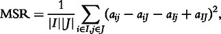where a_ij is the data element at row i and column j; a_iJ, a_Ij and a_IJ are the mean of the expression values in of row i, column j, and the whole bicluster respectively, for i ∈ I and j ∈ J. MSR was shown to be successful at finding constant biclusters, constant row and column biclusters, and shift biclusters. However, this metric is not suitable for scale and shift-scale biclusters [32, 20]. The algorithm starts with the whole data matrix removing the rows and the columns that have high residues. Once the MSR of the bicluster reaches a given threshold parameter δ, the rows and columns with smaller residue than the bicluster residue are added back to the bicluster. If multiple biclusters are to be recovered, the found biclusters are masked with random values, and the process repeats.

Order-preserving submatrix problem

OPSM is a deterministic greedy algorithm that seeks biclusters with ordered rows [23]. The OPSM model defines a bicluster as an order-preserving submatrix, in which there exists a linear ordering of the columns in which the expression values of all rows of that submatrix linearly increase. It can be shown that constant columns, shifting, scaling and shift-scale bicluster models are all order-preserving. OPSM constructs complete biclusters by iteratively growing partial biclusters, scoring each by the probability that it will grow to some fixed target size. Only the best partial biclusters are kept each iterations.

Conserved gene expression motifs

xMOTIFs is a nondeterministic greedy algorithm that seeks biclusters with conserved rows in discretized dataset [26]. For each row, the intervals of the discretized states are determined according to the statistical significance of the interval compared with the uniform distribution. For each randomly selected column, called a seed, and for each randomly selected set of columns, called discriminating sets, xMOTIFs tries to find rows that have same states over the columns of the seed and the discriminating set. Therefore, xMOTIFs can find biclusters with constant values at rows.

Qualitative biclustering

QUBIC is a deterministic algorithm that reduces the biclustering problem to finding heavy subgraphs in a bipartite graph representation of the data [30]. It seeks biclusters with nonzero constant columns in discrete data. The data are first discretized into down and upregulated ranks, then biclusters are generated by iterative expansion of a seed edge. The first expansion step requires that all columns be constant; in the second step this requirement is relaxed to allow the addition of rows that are not totally consistent.

BiMax

BiMax is a divide and conquer algorithm that seeks the rectangles of 1's in a binary matrix [14]. BiMax starts with the whole data matrix, recursively dividing it into a checker board format. Since the algorithm works only on binary data, datasets must first be converted, or binarized. In our experiments, thresholding was used: expression values higher than the given threshold were set to 1, the others to 0. The threshold for the binarization method was chosen as the mean of the data; therefore, BiMax is expected to find only upregulated biclusters. In our experiments, BiMax was also told the exact size of the expected biclusters, because otherwise it would halt prematurely, recovering only a small portion of the expected biclusters.

Iterative signature algorithm

Iterative signature algorithm (ISA) is a nondeterministic greedy algorithm that seeks biclusters with two symmetric requirements [24]: each column in the bicluster must have an average value above some threshold T_C; likewise each row must have an average value above some threshold T_R. The algorithm starts with a seed bicluster consisting of randomly selected rows. It iteratively updates the columns and rows of the bicluster until convergence. By re-running the iteration step with different row seeds, the algorithm finds different biclusters. ISA can find upregulated or downregulated biclusters.

Combinatorial algorithm for expression and sequence-based cluster extraction

Combinatorial algorithm for expression and sequence-based cluster extraction (COALESCE) is a nondeterministic greedy algorithm that seeks biclusters representing regulatory modules in genetics [28]. This algorithm can find upregulated and downregulated biclusters. It begins with a pair of correlated genes, then iterates, updating columns and rows until convergence. It select columns by two-population z-test, motifs by a modified z-test, and then selects rows by posterior probability. Although the algorithm was proposed to work on microarray data together with sequence data, sequence data was not used in the experiments. COALESCE was used with the default parameters in the experiments.

Plaid

Plaid fits parameters to a generative model of the data known as the plaid model [22]: a data element X_ij, with K biclusters assumed present, is generated as the sum of a background effect θ, cluster effects μ, row effects α, column effects β and random noise e:

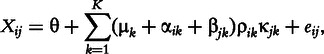where the background refers to any matrix element that is not a member of any bicluster. The Plaid algorithm fits this model by iteratively updating each parameter of the model to minimize the MSE between the modeled data and the true data.

Bayesian biclustering

Bayesian biclustering (BBC) uses Gibbs sampling to fit a hierarchical Bayesian version of the plaid model [27]. It restricts overlaps to occur only in rows or columns, not both, so that two biclusters may not share the same data elements. The sampled posteriors for cluster membership of each row and column represent fuzzy membership; thresholding yields crisp clusters.

Correlated pattern biclusters

Correlated pattern biclusters (CPB) is a nondeterministic greedy algorithm that seeks biclusters with high row-wise correlation according to the Pearson Correlation Coefficient (PCC) [29]. CPB starts with a reference row and a randomly selected set of columns. It iteratively adds the rows that have a high correlation, above the given PCC threshold parameter, with the average bicluster row, and columns that have smaller root mean squared error (RMSE) than the RMSE of the row that has smallest correlation. Various biclusters are found by random seeding of reference row and columns. This algorithm can find row shift and scale patterns.

Factor analysis for bicluster acquisition

Factor analysis for bicluster acquisition (FABIA) models the data matrix X as the sum of p biclusters plus additive noise ϒ, where each bicluster is the outer product of two sparse vectors [31]: a row vector λ and a column vector z:

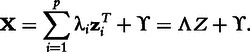Two factor analysis models are used to fit this model to the data set; variational expectation maximization is used to maximize the posterior. Row and column membership in each bicluster is fuzzy, but thresholds may be used to make crisp clusters. In all experiments, FABIA was thresholded to return crisp clusters.

Spectral biclustering

Spectral uses singular value decomposition to find a checkerboard pattern in the data in which each bicluster is up- or downregulated [25]. Only biclusters with variance lower than a given threshold are returned.

METHODS

Experiments were performed using BiBench (Available at http://bmi.osu.edu/hpc/software/bibench), a Python package for bicluster analysis developed by our lab. Implementations for all 12 algorithms were obtained from the authors. BiBench also depends on many Bioconductor packages [33], which are cited throughout the section.

Parameters

Choosing the correct parameters for each algorithm is crucial to that algorithm's success, but too often default parameters are used when comparing algorithms. We chose parameters specifically for the synthetic and GDS data that worked better than the defaults.

For synthetic datasets, all algorithms that find a specific number of biclusters were given the true number of biclusters. Those that generate multiple seeds were given 300 seeds. For GDS datasets, those same algorithms were given 30 biclusters and 500 seeds, respectively, with two exceptions. Cheng and Church was given 100 biclusters, based on its author's recommendations. BBC, which calculates the Bayesian Information Criterion (BIC) for a clustering [34], was run multiple times on each GDS dataset, and the clustering with the best BIC was chosen. The number of clusters for each run was 30, 35, 40, 45 and 50.

BBC provides four normalization procedures, but no normalization worked best for constant biclusters. IQRN normalization worked best for the plaid model, so we chose to use IQRN on all tests, because BBC was designed to fit the plaid model.

Choosing the correct δ and α parameters are important for Cheng and Church's accuracy and running time. δ controls the maximum MBR in the bicluster, and so affects the homogeneity of the results. On synthetic data we were able to get good results with δ = 0.1, but on GDS data it needed to be increased. We used δ = e/2400, where e was the difference between the maximum and minimum values in the dataset. α is the coefficient for multiple row or column deletion in a particular step. It controls the tradeoff between running time and accuracy; the minimum α = 1 causes Cheng and Church to run as fast as possible. On synthetic data we were able to use α = 1.5, but for the much larger GDS data it had to be reduced to 1.2.

The accuracy of BiMax, xMOTIFs and QUBIC depends on how the data are discretized. xMOTIFs performed best on synthetic data discretized to a large number of levels; we used 50. As the levels decreased, so xMOTIFs' performance suffered. For BiMax, which requires binary data, we used the discretization method used for QUBIC with two levels. QUBIC also performed best on synthetic datasets with only two levels. On GDS data, QUBIC got better results with the default of 10 ranks.

The Spectral biclustering algorithm performed poorly on synthetic data until we reduced the number of eigenvalues to one, used bistochastization normalization and increased the within-bicluster variance to five. On GDS data, it got better results using log normalization and a much larger variance. It failed to return any biclusters until the within-bicluster variance was extremely large, so we set it to twice the number of rows in the dataset.

Synthetic data generation

Datasets were generated with the following parameters, except when one parameter was varied in an experiment: 500 rows, 200 columns, one biclusters with 50 rows and 50, no noise, no overlap. Datasets from six different models of biclustering were generated.

• Constant biclusters: biclusters with a constant expression level close to dataset mean. The constant expression values of the biclusters were chosen to be 0; background values were independent, identically-distributed (i.i.d.) draws from the standard normal: N(0, 1).

• Constant, upregulated biclusters: similar to the previous model, but biclusters had a constant expression level of 5.

• Shift-scale biclusters: each bicluster row is both shifted and scaled from some base row. Base row, shift and scale parameters, and background were all i.i.d. ∼ N(0, 1). Scaling with a positive number makes the row positively correlated with the base, whereas scaling with a negative number results in a negatively correlated row.

• Shift biclusters: similar to shift-scale, but scaling parameters always equal 1.

• Scale biclusters: similar to shift-scale, but shifting parameters always equal 0.

• Plaid model biclusters: an additive bicluster model first introduced in [22]. Each element X_ij, with K biclusters assumed present, is modeled as the sum of a background effect θ cluster effects μ, row effects α, column effects β and random noise e. ρ and κ are indicator variables for row i and column j membership in bicluster k:

  

  All effects were chosen i.i.d. ∼ N(0, 1).

Evaluating synthetic results

Biclusters on synthetic dataset were scored by comparing the set of found biclusters against the expected biclusters, using the following method, adapted from [14]. Let b₁ and b₂ be biclusters, and s(b₁, b₂) be some score function which compares biclusters. Without loss of generality assume that s assigns larger scores to similar biclusters and small scores to dissimilar ones. Then two sets of biclusters, M₁ and M₂, are compared by calculating the set score S(M₁, M₂) [14]:

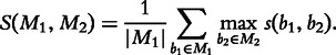Since S is not symmetric, it is used to define two scores, recovery and relevance, depending on the order of the expected and found biclusters. Let E denote the ground truth set of expected biclusters, and F denote the set of found biclusters. Recovery is calculated as S(E, F). It is maximized if E ⊆ F, i.e. if the algorithm found all of the expected biclusters. Similarly, relevance is calculated as S(F, E). It is maximized if F ⊆ E, i.e. all the found biclusters were expected.

In this article, s(b₁, b₂) was chosen to be the Jaccard coefficient applied to submatrix elements defined by each bicluster:

where |b₁ ∩ b₂| is the number of data elements in their intersection, and |b₁ ∪ b₂| is the number in their union. Identical biclusters achieve the largest score of s(b, b₂) = 1, and disjoint biclusters the lowest of s(b₁, b₂) = 0. Any score x ∈ [0, 1] is easily interpreted as the percentage x of total elements shared by both biclusters.

Evaluating GDS results

A different method must be used for evaluating the results of biclustering gene expression data, because the true biclusters are not known. Two classes of methods are available: internal and external. Internal measures of validity are based on intrinsic properties of the data and biclusters themselves, whereas external measures compare the biclusters to some other source of information. Since we compared a large number of algorithms, each fitting a different model, we chose to use external validation by calculating GO enrichment for the rows of each bicluster.

The enrichment analysis was carried out using the GOstats package [35]. Terms were chosen from the Biological Process Ontology. The genes associated with each probe in the bicluster were used as the test set; the genes associated with all the probes of each GDS dataset were chosen as the gene universe. Multiple test correction was performed using the Benjamini and Hochberg method [36]. Biclusters were considered enriched if the adjusted P-value for any gene ontology term was smaller than P = 0.05.

Most GDS datasets used in this work had missing values. These missing values were replaced using PCA imputation, provided by the pcaMethods package [37].

RESULTS

Model experiment

In previous comparative analysis studies, algorithms were compared on artificial data generated from a single model. However, each algorithm fits a different bicluster model. To compare algorithms on a single model often gives incomplete or misleading results. Instead, we evaluated each bicluster on synthetic datasets generated from six different models: constant, constant-upregulated, shift, scale, shift-scale and plaid.

Twenty datasets for each of the six models were generated, and each biclustering method was scored on each dataset. Plots of the mean recovery and relevance scores for all 20 datasets of each model are given in Figure 1.

Figure 1:

Bicluster model experiment. Each data point represents the average recovery vs. relevance scores of twenty datasets. A score of (1, 1) is best.

BiMax and OPSM do not filter their results, so they each return many spurious biclusters that hurt their relevance scores. However, our framework BiBench provides a bicluster filtering function that removes biclusters based on size and overlap with other biclusters. After filtering out the smaller one when the overlap between a pair of biclusters is at least 25%, their relevance scores were greatly improved (Figure 2).

Figure 2:

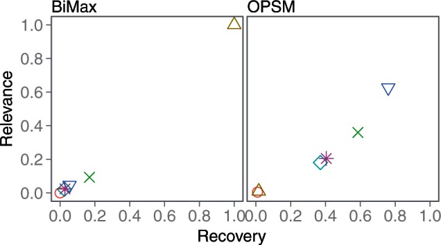
Results of bicluster model experiment after filtering. Each data point represents the average recovery vs. relevance scores of twenty datasets. A score of (1, 1) is best.

All algorithms were not expected to perform well on all datasets. Most algorithms were able to recover biclusters that fit their model, but there were a few exceptions.

BBC's results are sensitive to which normalization procedure it uses. Depending on the procedure chosen, it is capable of achieving perfect scores on constant, constant-upregulated, shift and plaid biclusters. We chose to use IQRN normalization, which maximized its performance on plaid-model biclusters.

Cheng and Church was expected to find any biclusters with constant expression value, but it could not find upregulated constant biclusters. We hypothesize that rows and columns with large expression values were pruned early because they increased the MSR of the candidate bicluster.

Since all the biclusters except constant and constant-upregulated were instances of order-preserving submatrices, OPSM was expected to succeed on these datasets. However, it did not perform well on scale or shift-scale biclusters. These failures are due to OPSM's method of scoring partial biclusters: it awards high scores for large gaps between expression levels, so biclusters with small or nonexistent gaps get pruned early in the search process. In these datasets, scale and shift-scale biclusters had small gaps because the scaling factors for each row were drawn from a standard normal distribution, contracting most rows toward zero and thus shrinking the gap statistic.

CPB was expected to do well on both constant and upregulated bicluster models. However, as the bicluster upregulation increased, CPB's recovery decreased. This behavior makes sense because CPB finds biclusters with high row-wise correlation. Increasing the bicluster upregulation also increases the correlation between any two rows of the data matrix that contain upregulated portions. Generating more bicluster seeds allowed CPB to recover the constant-upregulated biclusters.

FABIA only performed well on constant-upregulated biclusters, but it is important to note that it is capable of finding other bicluster models not represented in this experiment. The parameters for these datasets were generated from Gaussian distributions, whereas FABIA is optimized to perform well on data generated from distributions with heavy tails.

Some algorithms also performed unexpectedly well on certain data models. COALESCE, ISA and QUBIC were able to partially recover plaid-model biclusters by recovering the upregulated portions. BBC was able to partially recover shift-scale patterns.

In subsequent experiments, each algorithm was tested on datasets generated from the biclustering model on which it performed best in this experiment. Most did best on constant-upregulated biclusters. CPB and OPSM did best on shift biclusters, BBC on plaid-model biclusters, and Cheng and Church on constant biclusters.

Noise experiment

Data are often perturbed both by noise inherent in the system under measurement and by errors in the measuring process. The errors introduced from these sources lead to noisy data, in which some or all of the signal has been lost. Algorithms robust with respect to noise are preferable for any data analysis task. Therefore, the biclustering algorithms were compared on their ability to resist random noise in the data. Each dataset was perturbed by adding noise generated from a Gaussian distribution with zero mean and a varying standard deviation ϵ: N(0, ϵ). The results for noise experiment are given in the top row of Figure 3.

Figure 3:

Synthetic experiments: noise, number of biclusters and overlapping biclusters. Thick middle dot represents the mean score; lines show standard deviation.

As expected, increasing the random noise in the dataset negatively affected both the recovery and relevance of clustering returned by most algorithms. COALESCE, FABIA and Plaid were unaffected, and QUBIC was unaffected until the standard deviation of the error reached 1.0. ISA's recovery was unaffected, but the relevance of its results did suffer as the noise level increased.

In general, the algorithms which seek local patterns (Cheng and Church, CPB, OPSM, and xMOTIFs) were more sensitive to noise, whereas the algorithms that fit a model of the entire dataset (ISA, FABIA, COALESCE, Plaid, Spectral) were much less sensitive. We hypothesize that modeling the entire dataset makes most algorithms more robust because it uses all the available information in the data. There were exceptions to this pattern, however. BiMax and QUBIC both handled noise much better than did other algorithms that seek local patterns; we used QUBIC's method for binarizing the dataset for BiMax, which may have helped. BBC and Spectral fit global models, but both were affected by the addition of noise. Spectral, though affected, did perform better than most local algorithms. BBC was the only algorithm tested on plaid-model biclusters in this experiment, which may have contributed to its performance. OPSM is especially sensitive to noise because even relatively small perturbations may affect the ordering of rows. We hypothesized that xMOTIFs's poor performance was due to the large number of levels used when discretizing the data, but reducing the number of levels did not improve its score.

Number experiment

Most gene expression datasets are not likely to have only one bicluster. Large datasets with hundreds of samples and tens of thousands of probes may have hundreds or thousands of biclusters. Therefore, in this experiment, the algorithms were tested on their ability to find increasing numbers of biclusters. The datasets in this experiment had 250 columns; the number of biclusters varied from 1 to 5. The results are given in the middle row of Figure 3.

BBC, COALESCE, CPB, ISA, QUBIC and xMOTIFs were unaffected by the number of biclusters. In fact, CPB's, ISA's and xMOTIFs's relevance scores actually improved as the number of biclusters in the dataset increased.

Even when the number of biclusters is known, recovering them accurately can be challenging, as evidenced by the trouble the other algorithms had as the number increased. Plaid and OPSM were most affected, whereas the degradation in other algorithms' performances was more gradual.

These scores were calculated with the raw results after filtering as described before, ISA's recovery and relevance scores dropped to 0.25 when more than one bicluster was present. This behavior was caused by ISA finding a large bicluster that was a superset of all the planted biclusters.

Overlap experiment

Algorithms were also tested on their ability to recover overlapping biclusters. The overlap datasets were generated with two embedded biclusters, each with 50 rows and 50 columns. In each dataset, bicluster rows and columns overlapped by 0, 10, 20 and 30 elements. Past this point, the biclusters become increasingly indistinguishable, and so the recovery and relevance scores approach those for datasets with one bicluster.

The bicluster expression values in overlapping regions were not additive, with the exception of the plaid model. Shift biclusters were generated by choosing the shift and scale parameters in a way to let two biclusters have the same expression values at overlapping areas. The results are given in last row of Figure 3.

A few algorithms were relatively unaffected by overlap. ISA's scores did not change, Plaid's scores actually improve until the overlap degree reaches 30. CPB's relevance score dropped slightly, but it was otherwise unaffected.

OPSM's recovery scores increased, but only because its initial score was low, suggesting that it could only find one bicluster. As the overlapping area increases, it also boosts the recovery score.

Most other algorithms' scores were negatively affected by overlapping the biclusters. In particular, Spectral's scores plummeted; most other algorithms' scores decreased gradually. BBC's drop in score was expected, because it actually fits a modified plaid model that does not allow overlapping biclusters.

Runtime experiment

Since the biclustering task is NP-hard, algorithms must make tradeoffs between quality and computational complexity. The nature of these tradeoffs affects their runtime efficiency, which is especially relevant for analyzing large datasets. Therefore in this experiment the algorithms' running times were compared.

The results in Figure 4 gives the running times of the algorithms with increasing number of rows. Note that the algorithms used in this test have been implemented in different languages, with different levels of optimization; therefore, these results do not reflect their actual computational complexity. However, the efficiency of existing implementations is of practical interest for evaluating which algorithm to use.

Figure 4:

Running time of the algorithms with increasing number of rows. Note that y-axis is in log₂ scale.

The algorithms are tested on a computer with 2.27 GHz dual quad-core Intel Xeon CPUs, and 48 GB main memory. Almost all of the algorithms had linear running time curves on the log-log plot, indicating exponential growth. OPSM was the slowest for smaller datasets, but Cheng and Church's running time grew faster and overtook it. For larger datasets, xMOTIFs, ISA, BBC took the most time to finish.

GDS data

Algorithms were compared on eight gene expression datasets from the GEO database [1]: GDS181, GDS589, GDS1027, GDS1319, GDS1406, GDS1490, GDS3715 and GDS3716. The datasets are summararized in Table 1.

Table 1:

GDS datasets

Dataset	Genes	Samples	Description
GDS181	12559	84	Human and mouse
GDS589	8799	122	Rat peripheral and brain regions
GDS1027	15866	154	Rat lung SM exposure model
GDS1319	22548	123	C blastomere mutant embryos
GDS1406	12422	87	Mouse brain regions
GDS1490	12422	150	Mouse neural and body tissue
GDS3715	12559	110	Human skeletal muscles
GDS3716	22215	42	Breast epithelia: cancer patients

The number of biclusters found and enriched for each algorithm is given in Table 2. Biclusters were considered enriched if at least one term from the Biological Process Gene Ontology was enriched at the P = 0.05 level after Benjamini and Hochberg multiple test correction [36]. The last column in Table 2 shows the number of enriched biclusters after filtering out biclusters that overlapped by more than 25%. For instance, none of BBC's enriched biclusters overlapped, but only 20 of BiMax's were sufficiently different. CPB found the most enriched biclusters, both before and after filtering. Although some algorithms found more enriched biclusters than others, further work is required to fully explore those biclusters and ascertain their biological relevance. It is important to note that COALESCE was designed to use genetic sequence data in conjunction with gene expression data, but sequence data was not used in this test. Figure 5 gives the proportions of the filtered enriched biclusters for each algorithm and different significance levels (The proportions of the filtered biclusters for individual real datasets can be found at http://bmi.osu.edu/hpc/data/Eren12BiB_suppl/).

Table 2:

Aggregated results on all eight GDS datasets

Algorithm	Found	Enriched	Enriched filtered
BBC	285	96	96
BiMax	654	165	20
Cheng and Church	800	89	89
COALESCE	570	266	60
CPB	1312	463	404
FABIA	229	69	54
ISA	82	42	10
OPSM	126	47	20
Plaid	37	17	17
QUBIC	108	36	36
Spectral	415	201	59
xMOTIFs	144	30	30

Biclusters were considered enriched if any GO term was enriched with P = 0.05 level after multiple test correction. The set of enriched biclusters was filtered to allow at most 25% overlap by area.

Figure 5:

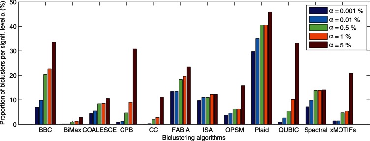
Proportion of the enriched biclusters for different algorithms on five different significance level (α). The results of eight real dataset are aggregated.

A full analysis of all the biclusters is outside the scope of this article, but we examined the best biclusters found by each algorithm. All 12 algorithms found enriched biclusters in GDS589. The terms associated with the bicluster with the lowest p-value for each algorithm are given in Table 3. The results are suggestive, considering that GDS589 represents gene expression of brain tissue. Most biclusters were enriched with terms related to protein biosynthesis. CPB's bicluster contained proteins involved with the catabolism of l-phenylalanine, an essential amino acid linked with brain development disorders in patients with phenylketonuria [38]. OPSM found a bicluster with almost 400 genes enriched with anti-apoptosis and negative regulation of cell death terms, which are important for neural development [39]. Similarly, QUBIC's bicluster was enriched with terms involving cell death and gamete generation. xMOTIFs and ISA both found biclusters enriched with RNA processing terms. BBC, COALESCE and Spectral all found biclusters enriched with glycolosis, glucose metabolism and hexose catabolism. These are interesting especially because mammals' brains typically use glucose as their main source of energy [40].

Table 3:

Five most enriched terms for each algorithm's best bicluster on GDS589

Algorithm	Rows, cols	Terms (P-value)
BBC	94, 117	Translational elongation (2.00e-30)
		Cellular biosynthetic process (1.38e-06)
		Glycolysis (7.37e-06)
		Hexose catabolic process (3.64e-05)
		Macromolecule biosynthetic process (1.20e-04)
BiMax	42, 9	Chromatin assembly or disassembly (2.75e-02)
Chng&Chrch	539, 91	Epithelial tube morphogenesis (9.94e-04)
		Branching inv. in ureteric bud morphogenesis (4.26e-02)
		Morphogenesis of a branching structure (4.26e-02)
		Organ morphogenesis (4.26e-02)
		Response to bacterium (4.26e-02)
COALESCE	103, 122	Translational elongation (6.75e-12)
		Glycolysis (2.88e-03)
		Energy derivation by ox. of organic cmpnds (5.57e-03)
		Hexose catabolic process (5.57e-03)
		ATP synthesis coupled electron transport (1.47e-02)
CPB	229, 98	Oxoacid metabolic process (2.83e-13)
		Oxidation-reduction process (2.72e-08)
		Cellular amino acid metabolic process (4.82e-04)
		Monocarboxylic acid metabolic process (2.63e-03)
		L-phenylalanine catabolic process (1.30e-02)
FABIA	56, 28	Translational elongation (3.22e-17)
		Macromolecule biosynthetic process (2.99e-06)
		Protein metabolic process (4.12e-05)
		Translation (4.12e-05)
		Cellular macromolecule metabolic process (2.12e-04)
ISA	292, 11	Translational elongation (1.44e-65)
		Protein metabolic process (5.35e-12)
		RNA processing (2.26e-09)
		Biosynthetic process (4.19e-09)
		rRNA processing (1.47e-08)
OPSM	378, 11	Multicellular organism reproduction (2.78e-04)
		Gamete generation (1.31e-03)
		Neg. regulation of programmed cell death (2.92e-03)
		Spermatogenesis (6.90e-03)
		Anti-apoptosis (4.31e-02)
Plaid	22, 15	Translational elongation (6.29e-30)
		Macromolecule biosynthetic process (1.78e-10)
		Protein metabolic process (3.13e-09)
		Cellular biosynthetic process (9.09e-08)
		Cellular macromolecule metabolic process (1.60e-06)
QUBIC	40, 8	Gamete generation (1.95e-02)
		Death (1.99e-02)
		Regulation of cell death (3.55e-02)
		Neg. rgltn. DNA damage response … p53 … (4.64e-02)
		Neg. rgltn of programmed cell death (4.64e-02)
Spectral	192, 73	Glycolysis (1.08e-05)
		Organic acid metabolic process (1.08e-05)
		Glucose metabolic process (4.51e-05)
		Hexose catabolic process (4.51e-05)
		Monosaccharide metabolic process (6.89e-05)
xMOTIFs	50, 7	Translational elongation (7.89e-12)
		ncRNA metabolic process (2.76e-03)
		rRNA processing (3.51e-03)
		Cellular protein metabolic process (1.23e-02)
		Anaphase-promoting … catabolic process (2.63e-02)

Key Points.

• Choosing the correct parameters for each algorithm was crucial. Many similar publications used default parameters, which often yielded poor results in this study. Some algorithms, like Cheng and Church, may also exhibit excessive running time if parameters are not chosen carefully.

• Algorithms that model the entire dataset seem more resilient to noise than algorithms that seek individual biclusters.

• The performance of most algorithms tested in this article degraded as the number of biclusters in the dataset increased. This is especially a concern for large gene expression datasets, which may contain hundreds of biclusters.

• No algorithm was able to fully separate biclusters with substantial overlap.

• In gene expression data, all algorithms were able to find biclusters enriched with GO terms. CPB found the most, followed by BBC. Surprisingly, the oldest of the biclustering algorithms, Cheng and Church, found the third most number of enriched biclusters. Although Plaid finds very few biclusters, it finds the highest proportion of enriched biclusters.

• Performance on synthetic datasets did not always correlate with performance on gene expression datasets. For instance, the Spectral algorithm was highly sensitive to noise, number of biclusters, and overlap in synthetic data, but was able to find many enriched biclusters in gene expression data.

• As expected, each algorithm performed best on different biclustering models. Before concluding that one algorithm outperforms another, it is important to consider the kind of data on which they were compared. On plaid biclusters BBC is the best performing algorithm. For constant-upregulated biclusters, COALESCE, FABIA, ISA, Plaid, QUBIC, xMOTIFs and BiMax are the alternatives. Among these algorithms, Plaid and QUBIC have the highest enriched bicluster ratio in real datasets. For constant, scale, shift and shift-scale datasets, CPB is the best performing algorithm. Moreover, when negative correlation is sought, the algorithms that perform well on scale and shift-scale biclusters can be used. However, most of the time the desired bicluster model is unknown, therefore the algorithms that work well in various models (e.g. CPB, Plaid and BBC) can be preferred. These algorithms also obtain good results on real datasets. While CPB and BBC find the most enriched biclusters, Plaid was able to obtain the highest proportion of enriched biclusters.

FUNDING

This work was supported in parts by the National Institutes of Health/National Cancer Institute [R01CA141090]; by the Department of Energy SciDAC Institute [DE-FC02-06ER2775]; and by the National Science Foundation [CNS-0643969, OCI-0904809, OCI-0904802].

Biographies

Kemal Eren is an MS student in the Department of Computer Science and Engineering at The Ohio State University.

Mehmet Deveci PhD student in the Department of Computer Science and Engineering at The Ohio State University.

Onur Küçüktunç PhD student in the Department of Computer Science and Engineering at The Ohio State University.

Ümit V. Çatalyürek Associate Professor in the Departments of Biomedical Informatics and Electrical and Computer Engineering at The Ohio State University.

References

- 1.Edgar R, Domrachev M, Lash AE. Gene Expression Omnibus: NCBI gene expression and hybridization array data repository. Nucleic Acids Research. 2002;30(1):207–10. doi: 10.1093/nar/30.1.207. [DOI] [PMC free article] [PubMed] [Google Scholar]
- 2.Hartigan JA. Direct clustering of a data matrix. J Am Stat Assoc. 1972;67(337):123–9. [Google Scholar]
- 3.Cheng Y, Church GM. Proceedings 8th International Conference Intelligent Systems for Molecular Biology. AAAI Press; 2000. Biclustering of expression data; pp. 93–103. [PubMed] [Google Scholar]
- 4.Madeira SC, Oliveira AL. Biclustering algorithms for biological data analysis: a survey. IEEE/ACM Trans Comput Biol Bioinformatics. 2004;1:24–45. doi: 10.1109/TCBB.2004.2. [DOI] [PubMed] [Google Scholar]
- 5.Tanay A, Sharan R, Shamir R. Chapman SA, editor. Biclustering algorithms: a survey. Handbook of Computational Molecular Biology. 2005 [Google Scholar]
- 6.Busygin S, Prokopyev O, Pardalos PM. Biclustering in data mining. Comput Operat Res. 2008;35:2964–87. [Google Scholar]
- 7.Fan N, Boyko N, Pardalos PM. Computational Neuroscience. Vol. 38. New York: Springer; 2010. Recent advances of data biclustering with application in computational neuroscience; pp. 105–32. [Google Scholar]
- 8.Madeira SC, Oliveira AL. A polynomial time biclustering algorithm for finding approximate expression patterns in gene expression time series. Algorithms Mol Biol. 2009;4(1):8. doi: 10.1186/1748-7188-4-8. [DOI] [PMC free article] [PubMed] [Google Scholar]
- 9.Van Mechelen I, Bock HH, De Boeck P. Two-mode clustering methods: a structured overview. Stat Methods Med Res. 2004;13(5):363–94. doi: 10.1191/0962280204sm373ra. [DOI] [PubMed] [Google Scholar]
- 10.Patrikainen A, Meila M. Comparing subspace clusterings. IEEE Trans Knowledge Data Eng. 2006;18:902–16. [Google Scholar]
- 11.Yoon S, Benini L, De Micheli G. Co-clustering: a versatile tool for data analysis in biomedical informatics. IEEE Trans Informat Technol Biomed. 2007;11(4):493–4. doi: 10.1109/titb.2007.897575. [DOI] [PubMed] [Google Scholar]
- 12.Kriegel HP, Kröger P, Zimek A. Clustering high-dimensional data: A survey on subspace clustering, pattern-based clustering, and correlation clustering. ACM Trans Knowledge Discov Data. 2009;3:1–58. [Google Scholar]
- 13.Turner H, Bailey T, Krzanowski W. Improved biclustering of microarray data demonstrated through systematic performance tests. Comput Stat Data Anal. 2005;48(2):235–54. [Google Scholar]
- 14.Prelić A, Bleuler S, Zimmermann P, et al. A systematic comparison and evaluation of biclustering methods for gene expression data. Bioinformatics. 2006;22(9):1122–9. doi: 10.1093/bioinformatics/btl060. [DOI] [PubMed] [Google Scholar]
- 15.Santamaría R, Quintales L, Therón R. Proceedings of 8th International conference Intelligent Data Engineering and Automated Learning. Heidelberg: Springer; 2007. Methods to bicluster validation and comparison in microarray data; pp. 780–9. [Google Scholar]
- 16.de Castro PAD, de Franca FO, Ferreira HM, et al. Proceedings of 7th International Conference Hybrid Intelligent Systems. Washington, DC: IEEE Computer Society; 2007. Evaluating the performance of a biclustering algorithm applied to collaborative filtering - a comparative analysis; pp. 65–70. [Google Scholar]
- 17.Wiedenbeck M, Krolak-Schwerdt S. Studies in Classification, Data Analysis and Knowledge Organization. Vol. 37. Heidelberg: Springer; 2009. ADCLUS: a data model for the comparison of two-mode clustering methods by Monte Carlo simulation; pp. 41–51. [Google Scholar]
- 18.Shepard RN, Arabie P. Additive clustering: Representation of similarities as combinations of discrete overlapping properties. Psychol Rev. 1979;86(2):87–123. [Google Scholar]
- 19.Filippone M, Masulli F, Rovetta S. Comput Intell Methods Bioinformatics Biostatistics. Vol. 5488 of LNCS. Berlin, Heidelberg: Springer; 2009. Stability and performances in biclustering algorithms; pp. 91–101. [Google Scholar]
- 20.Bozdağ D, Kumar A, Çatalyürek UV. Proceedings of 1st ACM International Conference Bioinformatics and Computational Biology. 2010. Comparative analysis of biclustering algorithms; pp. 265–74. [Google Scholar]
- 21.Chia BK, Karuturi RK. Differential co-expression framework to quantify goodness of biclusters and compare biclustering algorithms. Algorithms Mol Biol. 2010;5:23. doi: 10.1186/1748-7188-5-23. [DOI] [PMC free article] [PubMed] [Google Scholar]
- 22.Lazzeroni L, Owen A. Plaid models for gene expression data. Stat Sin. 2000;12:61–86. [Google Scholar]
- 23.Ben-Dor A, Chor B, Karp R, et al. Discovering local structure in gene expression data: the order-preserving submatrix problem. J Comput Biol. 2003;10(3-4):373–84. doi: 10.1089/10665270360688075. [DOI] [PubMed] [Google Scholar]
- 24.Bergmann S, Ihmels J, Barkai N. Iterative signature algorithm for the analysis of large-scale gene expression data. Phys Rev E. 2003;67(3 Pt 1):031902. doi: 10.1103/PhysRevE.67.031902. [DOI] [PubMed] [Google Scholar]
- 25.Kluger Y, Basri R, Chang JT, et al. Spectral biclustering of microarray data: coclustering genes and conditions. Genome Res. 2003;13(4):703–16. doi: 10.1101/gr.648603. [DOI] [PMC free article] [PubMed] [Google Scholar]
- 26.Murali TM, Kasif S. Extracting conserved gene expression motifs from gene expression data. Pacific Symposium of Biocomputing. 2003:77–88. [PubMed] [Google Scholar]
- 27.Gu J, Liu JS. Bayesian biclustering of gene expression data. BMC Genomics. 2008;9(Suppl 1):S4. doi: 10.1186/1471-2164-9-S1-S4. [DOI] [PMC free article] [PubMed] [Google Scholar]
- 28.Huttenhower C, Mutungu KT, Indik N, et al. Detailing regulatory networks through large scale data integration. Bioinformatics. 2009;25(24):3267–3274. doi: 10.1093/bioinformatics/btp588. [DOI] [PMC free article] [PubMed] [Google Scholar]
- 29.Bozdağ D, Parvin JD, Çatalyürek UV. Proceedings 1st International Conference Bioinformatics and Computational Biology. Berlin, Heidelberg: Springer-Verlag; 2009. A biclustering method to discover co-regulated genes using diverse gene expression datasets; pp. 151–63. [Google Scholar]
- 30.Li G, Ma Q, Tang H, et al. QUBIC: a qualitative biclustering algorithm for analyses of gene expression data. Nucleic Acids Res. 2009;37(15):e101. doi: 10.1093/nar/gkp491. [DOI] [PMC free article] [PubMed] [Google Scholar]
- 31.Hochreiter S, Bodenhofer U, Heusel M, et al. FABIA: factor analysis for bicluster acquisition. Bioinformatics. 2010;26(12):1520–27. doi: 10.1093/bioinformatics/btq227. [DOI] [PMC free article] [PubMed] [Google Scholar]
- 32.Aguilar-Ruiz J. Shifting and scaling patterns from gene expression data. Bioinformatics. 2005;21(20):3840–5. doi: 10.1093/bioinformatics/bti641. [DOI] [PubMed] [Google Scholar]
- 33.Gentleman RC, Carey VJ, Bates DM, et al. Bioconductor: open software development for computational biology and bioinformatics. Genome Biol. 2004;5(10):R80. doi: 10.1186/gb-2004-5-10-r80. [DOI] [PMC free article] [PubMed] [Google Scholar]
- 34.Schwarz G. Estimating the dimension of a model. Ann Stat. 1978;6(2):461–4. [Google Scholar]
- 35.Falcon S, Gentleman RC. Using GOstats to test gene lists for GO term association. Bioinformatics. 2007;23(2):257–8. doi: 10.1093/bioinformatics/btl567. [DOI] [PubMed] [Google Scholar]
- 36.Hochberg Y, Benjamini Y. More powerful procedures for multiple significance testing. Stat Med. 1990;9(7):811–8. doi: 10.1002/sim.4780090710. [DOI] [PubMed] [Google Scholar]
- 37.Stacklies W, Redestig H, Scholz M, et al. pcaMethods–a bioconductor package providing PCA methods for incomplete data. Bioinformatics. 2007;23(9):1164–7. doi: 10.1093/bioinformatics/btm069. [DOI] [PubMed] [Google Scholar]
- 38.Pietz J, Kreis R, Rupp A, et al. Large neutral amino acids block phenylalanine transport into brain tissue in patients with phenylketonuria. J Clin Investigat. 1999;103(8):1169–78. doi: 10.1172/JCI5017. [DOI] [PMC free article] [PubMed] [Google Scholar]
- 39.White LD, Barone S. Qualitative and quantitative estimates of apoptosis from birth to senescence in the rat brain. Cell Death Diff. 2001;8(4):345–56. doi: 10.1038/sj.cdd.4400816. [DOI] [PubMed] [Google Scholar]
- 40.Karbowski J. Global and regional brain metabolic scaling and its functional consequences. BMC Biol. 2007;5:18. doi: 10.1186/1741-7007-5-18. [DOI] [PMC free article] [PubMed] [Google Scholar]