

Abstract
Objective
The steady-state visual evoked potential (SSVEP) is an electroencephalographic response to flickering stimuli generated partly in primary visual area V1. The typical “cruciform” geometry and retinotopic organization of V1 is such that certain neighboring visual regions project to neighboring cortical regions of opposite orientation. Here, we explored ways to exploit this organization in order to boost scalp SSVEP amplitude via oscillatory summation.
Approach
We manipulated flicker-phase offsets among angular segments of a large annular stimulus in three ways, and compared the resultant SSVEP power to a conventional condition with no temporal phase offsets. 1) we divided the annulus into standard octants for all subjects, and flickered upper horizontal octants with opposite temporal phase to the lower horizontal ones, and left vertical octants opposite to the right vertical ones; 2) we individually adjusted the boundaries between the 8 contiguous segments of the standard octants condition to coincide with cruciform-consistent, early-latency topographical shifts in pattern-pulse multifocal visual-evoked potentials (PPMVEP) derived for each of 32 equal-sized segments; 3) we assigned phase offsets to stimulus segments following an automatic algorithm based on the relative amplitudes of vertically- and horizontally-oriented PPMVEP components.
Main results
The three flicker-phase manipulations resulted in a significant enhancement of normalized SSVEP power of 1) 202%, 2) 383%, and 3) 300%, respectively.
Significance
We have thus demonstrated a means to obtain more reliable measures of visual evoked activity purely through consideration of cortical geometry. This principle stands to impact both basic and clinical research using SSVEPs.
1. Introduction
Scalp electroencephalography (EEG) has been widely used as a means to record neural activity noninvasively from the human cerebral cortex with high temporal resolution. Visual evoked potentials (VEP) are extrinsically induced EEG potentials that appear over the occipital lobe in response to a discrete visual event. When a stimulus is presented repetitively at a rate ranging from approximately 7 Hz to 60 Hz (Regan 1977), the brain’s visual response reaches a steady state, and generates a phase-locked oscillation at the same (fundamental) frequency as the visual stimulus and/or at multiples (harmonics) thereof, known as the Steady State Visually Evoked Potential (SSVEP; Regan 1989).
SSVEPs have many applications in neural engineering and neuroscience. Simply by computing the Fourier Transform of EEG time segments, the magnitude and phase spectra of the SSVEP can be obtained in the frequency domain. The peak amplitude or power at the frequency of stimulation provides a robust measure of the intensity of sensation for the stimulus “tagged” by that frequency. For that reason, SSVEPs popularly serve as inputs to gaze-dependent (Wang et al 2005, Gao et al 2003) and gaze-independent (Kelly et al 2005a, b; Allison et al 2008) brain-computer interfaces (BCI), allowing communication between motor impaired patients and their environment (Wolpaw et al 2002; Allison et al 2007), and have been a highly useful tool in cognitive neuroscience research. For example, SSVEPs provide a measure of the modulation of visual activity by spatial (Morgan et al 1996, Muller et al 2003, Lauritzen et al 2010), feature-based (Anderson and Muller 2010) and intersensory (Saupe et al 2009) attention, and a means to track sensory evidence over time during perceptual decision formation (O’Connell et al 2012).
As with all signals in human electrophysiology, the SSVEP is enveloped in a considerable amount of noise, greatly limiting our ability to obtain robust measurements on a single-trial basis. The problem of noise is exacerbated in conditions under which SSVEP amplitude is low, such as when the flicker frequency is high (>20 Hz), when stimuli are in the visual periphery, and/or when low contrast stimuli are used. These very conditions are of significant interest in many lines of basic and applied vision research, leading to an imperative to improve SSVEP signal-to-noise ratio (SNR). Strides on this front have been made especially in the BCI field. Some studies have employed individual optimization of stimulus parameters such as temporal and spatial frequency to maximize SNR (Lopez-Gordo et al 2011). Other studies use more complex multivariate transformations or array decompositions to increase the SNR of the SSVEP (Cichocki et al 2008).
The aim of the current study was to quantify the improvement in SSVEP SNR attained solely by exploiting individual primary visual cortex (V1) geometry, without the use of any signal transformations beyond the standard Fast Fourier Transform (FFT). As the first cortical area that receives retinal input, V1 is thought to contribute significantly to the amplitude of the SSVEP on the scalp, and the results of source localization studies support this notion (e.g. Di Russo et al 2007; Lauritzen et al 2010). In humans, area V1 lies predominantly on the medial occipital cortical surface, covering an area that includes the calcarine sulcus and its outer banks. Its geometry and retinotopic organization generally follows a well-known “cruciform” configuration, whereby the upper and lower horizontal field octants of visual space project to the floor and ceiling of the contralateral calcarine sulcus, respectively, while the upper and lower vertical field octants project to the ventral and dorsal medial surface on the lips of the calcarine sulcus (Holmes 1945; Jeffreys and Axford 1972; see Figure 1a, b). As a result of this retinotopic organization, certain neighboring regions of space project to neighboring but oppositely-oriented sections of the cortical surface (Figure 1b). Thus, when facing regions are simultaneously activated, their electric fields will tend to cancel out. However, if oscillatory responses in these oppositely-facing regions are driven with opposite phase, constructive interference would be predicted to occur and produce larger SSVEPs on the scalp (Figure 1c, d).
Figure 1.

a- Visual field divided into symmetrical octants, paired with the ideal topographical distributions of the initial component (“C1”) of the transient VEP that would result from discrete stimulation at each location. Negative(−) and positive(+) scalp topographies represent the polarity of the initial VEP component. b- Coronal view of the calcarine sulcus located on the medial surface of the occipital lobe, illustrating the cruciform model of V1. Each arrow depicts electrical dipole orientation as a result of stimulation at the location in visual space of the corresponding color. c- Signal cancellation as a result of destructive interference between opposite dipoles being stimulated with temporally in-phase flicker stimuli. d- Signal summation as a result of constructive interference between opposite dipoles being stimulated temporally out-of phase.
In order to apply this constructive interference principle to enhance the SSVEP, we imposed temporal phase offsets among angular segments of a flickering annular pattern stimulus and compared the resultant amplitude to a “standard” condition in which the entire annulus flickered temporally in phase. In a first test condition (“symmetric”), we assumed a perfectly symmetrical, ideal cruciform configuration for all subjects as depicted in figure 1a,b, in which V1 is divided symmetrically into horizontal and vertical parallel-facing segments and discrete turns in the cortical surface correspond to polar angles at 45-degree increments in space. The upper horizontal octants were flickered with opposite temporal phase (180°) relative to the lower horizontal octants, and similarly the left vertical octants were flickered opposite to the right vertical octants, so that constructive interference should occur for both the vertically-oriented and horizontally-oriented dipolar electric fields.
In two further test conditions, we attempted to account for differences in visual cortex geometry across individuals. It is well known that area V1 varies widely in anatomical shape and extent (Brindley 1972, Stensaas et al 1974). Variability in cortical folding patterns and the distribution of V1 within the calcarine sulcus contributes substantially to subject-to-subject variability in the topographical variations of early VEP responses with respect to stimulus location (Jeffreys and Smith 1979, Butler et al 1987, Clark et al 1995). To characterize individual V1 geometry, we performed multifocal pattern-pulse stimulation at 32 radial segments of the annular stimulus. The pattern-pulse multifocal visual evoked potential (PPMVEP) is a technique that enables the simultaneous derivation of pattern-onset VEPs from multiple visual field locations by presenting orthogonal discrete pulse trains (James 2003) at each location. The resultant VEPs strongly depend on the retinal location of the stimulus and inherent anatomical differences across subjects. For our current purposes, we took the amplitude in the early time range of 80–90 ms of the PPMVEP as an index of V1 activity (Baseler et al 1994; Slotnick et al 1999; Fortune et al 2009). We assigned flicker phase-offsets to segments of the SSVEP stimulus in two ways: first, scalp topographies were visually inspected with reference to the typical source geometry of the cruciform model, and boundaries of the standard octants were adjusted to align with polar angles in the visual field where characteristic polarity inversions and topographical shifts of the VEP occurred (“tailored octants” condition). Second, phase offsets were computed using an automatic computer-based algorithm assigning each of the 32 segments to one of 4 phases (0°, 90°, 180°, 270°) based on the signs and relative magnitudes of horizontal and vertical dipolar PPMVEP components (“auto-phase assignment” condition). We quantified improvements in SSVEP SNR simply by calculating spectral power at the frequency of flickering in the standard Discrete Fourier Transform.
2. Materials and methods
1.1 Subjects
EEG data were recorded from 16 healthy subjects between 22 and 32 years old (8 female). All participants reported normal or corrected-to-normal vision and no history of neurological disorders. Informed consent was obtained before their participation, and all experimental procedures were approved by the Institutional Review Board of The City College of New York.
2.2 Stimuli
The procedure was conducted inside a dark, soundproof and radio frequency interference (RFI) shielded room. Stimuli were presented on a gamma-corrected CRT monitor (Dell M782) with a refresh rate of 85Hz and 1280x1024 pixels of resolution. Stimuli were presented dichoptically at a viewing distance of 57 cm. The background (middle) luminance was fixed at 64.39cd/m2 after estimating the gamma correction curve of luminance. Our stimulus presentation was programmed in a commercial software package (MATLAB 6.1, The MathWorks Inc., Natick, MA, 2000), with the PsychToolbox extension (Brainard 1997, Pelli 1997). A small white square was presented at the center of the screen during the full length of the experiment, as a fixation spot. Subjects were instructed to maintain fixation on this spot throughout each block, and this was monitored continually by the experimenter.
In each of the four stimulation conditions we presented a 100%-contrast, annular checkerboard stimulus with inner radius of 3° and outer radius of 10°, flickering at 21.25 Hz. We chose this frequency because it avoids highly reactive bands such as alpha and, as mentioned in the introduction, SNR is known to be lower at higher frequencies. The checkerboard was composed of 64 x 7 checks in total (polar angle x eccentricity). The conditions varied only in the way temporal phase was offset among radial segments of the pattern:
Standard. As a baseline comparison condition, we used a conventional configuration in which the entire annulus flickered temporally in phase (Figure 2a).
Symmetric. This configuration assumes a perfectly symmetric brain anatomy in which the calcarine sulcus contains ideally parallel-facing segments that perfectly map onto the horizontal octants. The annular checkerboard was divided into eight 45-degree segments, and the upper horizontal angular octants were flickered with opposite temporal phase relative to the lower horizontal ones. In the same manner, the left vertical octants were flickered with opposite phase relative to the right vertical ones (Figure 2b).
Tailored Octants. We attempted to account for variability in visual cortex geometry across individuals. To characterize individual geometry, we performed pattern-pulse multifocal stimulation of 32 radial segments of the annular stimulus derived from shifted versions of an original binary m-sequence (Baseler et al 1994; James 2003; see below section 2.4.). In the Tailored Octants condition, the 32 topographic maps were associated with approximate source orientations by visual inspection, using the standard cruciform model as a reference (Figure 1a,b). We adjusted the boundaries of the 8 octants to coincide with the transitions in PPMVEP topography from midline-focused to lateralized (shift from horizontally to vertically-oriented cortical surface), and from positive to negative polarity (shift from ceiling to floor of calcarine, or from left to right hemisphere). An individually-characterized visual stimulus configuration was thus formed, with the same flicker-phase assignments as the symmetric condition but without the constraint of equal size across the 8 segments (Figure 2c; see also Figure 3c for individual example).
Auto-Phase Assignment. From the same scalp topographic maps extracted from the PPMVEP, an automatic computer-based algorithm assigned each of the 32 segment responses to one of 4 phase offsets: 0°, 90°, 180° and 270°. In this case, there were intermingled segments flickering at shifted temporal phases (Figure 2d). The details of this algorithm are provided below.
Figure 2.
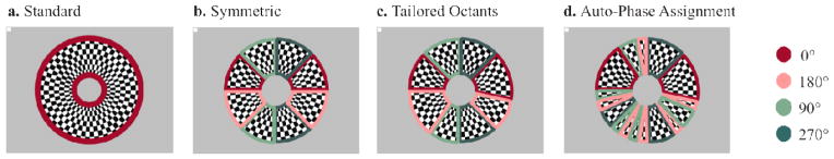
Flicker phase assignment schemes across the four SSVEP conditions of stimulation. The flicker frequency was 21.25 Hz in all cases. a- The Standard stimulus is the conventional configuration used for measuring SSVEPs whereby the entire annulus flickers in-phase (0° shift). b- Symmetric stimulus with segment boundaries placed at 45-degree increments in polar angle. Light and dark red octants are flickered with a temporal phase offset (180° shift) that leads to constructive interference on the scalp. In the same manner, the light and dark green octants are driven in opposite phase. c- Tailored Octants configuration based on scalp topographies obtained from the multifocal mapping. This appears highly similar to the standard octants condition but with boundaries adjusted to coincide with cruciform-consistent shifts in topography. Note for example that in this representative subject, whose PPMVEP topographies are shown in figure 3c, the transition from midline-negative to midline-positive topographies occurs one segment below the horizontal meridian in the right visual field. d- The automatic phase-assignment condition relies on an algorithm that assigns one of 4 possible phase offsets to each of the 32 segments based on the relative amplitude of horizontally-oriented and vertically-oriented neural response components.
Figure 3.

Pattern-pulse multifocal VEPs extracted as a response to each of the 32 locations in the visual field for one representative subject. a- PPMVEP waveforms from a single electrode in a single subject for all 32 locations, showing the time window in which the topographic maps were computed (80 to 90 ms). b- Vertical (V) and Horizontal (H) signals were extracted from the indicated pairs of electrode sets. These bipolar signal components were used both in the PPMVEP-based automatic phase assignment algorithm and in the measurement of SSVEP power in the main SSVEP stimulation conditions. c- Topographies of the earliest PPMVEP component for another representative subject, showing clear variations according to the location of the stimulus in the visual field. In the Tailored Octants condition, octant boundaries were determined by eye, and are indicated for this subject by brackets stemming from each corresponding ideal topography. In the Auto-Phase Assignment condition, phase offsets were assigned to segments automatically on the basis of the simple classification of H and V components in the coordinate system shown in the inset. Early signal amplitude for the “V” bipolar signal (red electrodes minus orange) is plotted against “H” amplitude (blue minus green) for each of the 32 segments. The dashed diagonal lines mark the boundaries between the four phase classes.
For all subjects the PPMVEP mapping procedure was administered first, lasting approximately 5 minutes, before any SSVEP recording. The SSVEP conditions were presented in separate blocks, which were run in counterbalanced order across subjects according to a Latin square. Each block contained 5 trials of the same SSVEP condition, each of them lasting 24 seconds resulting in a block duration of approximately 3 minutes. To avoid tiredness and eye fatigue, the subjects had a break of 15 minutes between the multifocal mapping and SSVEP testing. The total recording time was always less than 1 hour.
2.3 Data acquisition
EEG data were recorded from a 64-channel montage using Brain Products DC amps and the actiCAP system (Oostenveld and Praamstra 2001) with an online reference at standard site FCz. Data were collected at a sample rate of 500 Hz with an online notch filter at 60 Hz, and high-pass filter with 0.5-Hz cut-off. Impedances were stable below 30 k3. Data were analyzed offline in Matlab using in-house scripts in conjunction with data reading routines and topographic mapping functions of EEGLAB (an open source toolbox for EEG analysis; Delorme and Makeig 2004). Offline, we applied a band-pass Butterworth digital filter (4th order) with cut-off frequencies 1 and 45 Hz.
2.4 Multifocal mapping
The multifocal VEP technique enables the simultaneous derivation of VEPs from multiple visual field locations by applying orthogonal stimulus waveforms to drive phase-reversal (Baseler et al 1994; Slotnick et al 1999) or discrete pulse presentation (James 2003) at each location. The resultant VEPs strongly depend on the retinal location of the stimulus and inherent anatomical differences across subjects. Topographical maps of the initial VEP component (Figure 3c) thus provide a reliable window on the reversals and turns of the cortical surface and their corresponding boundaries in the visual field.
To establish how scalp topographies for a given individual vary as a function of polar angle in the visual field, we used the same annular checkerboard stimulus divided into 32 segments covering 3 to 10° of eccentricity and each spanning 11.25° of polar angle (3/16 rad, 2 x 7 checks). We converted an original binary m-sequence of length 1024 (composed of transitions between 1 and −1, with equal total time spent on each level) to a pulse train by designating every −1 to 1 transition as a pulse and setting all other frames to zero. We then interposed 3 blank frames between every frame to create a pulse sequence of 4096 frames, lasting 48s. Because the 32 pulse trains are orthogonal, visual evoked potentials can be estimated by deriving the impulse response function of the visual system to each segment using multiple linear regression (James 2003, Baseler et al 1994).
To assign phase offsets to stimulus segments based on these PPMVEP data in the “Auto-phase assignment” condition, we assumed a set of four distinct, ideal topographies (see Figures 1a and 3c) associated with the cruciform model, and matched each of the 32 measured topographies for a given individual to one of the ideal topographies. We computed topographic maps in the typical time range of the peak of the initial “C1” component of the VEP, 80 to 90 ms (Figure 3a; see e.g. Clark et al 1995). For the purposes of the present study, we took the scalp potential in this time window to reflect mainly V1 activity, in keeping with previous work using multifocal paradigms (e.g. Baseler et al 1994; Slotnick et al 1999; Park et al 2008; see Ales et al 2010, 2012 and Kelly et al 2012 for a fuller discussion). In the Tailored octants condition, we adjusted segment boundaries simply by visual inspection of these topographies. For the Auto-Phase Assignment condition, we decomposed this early visual response component into horizontal and vertical components using a simple cartesian coordinate system in order to capture activity from vertically- and horizontally-oriented sections of the cortical surface, respectively. Specifically, we derived a horizontal “H” signal by subtracting right hemisphere electrodes from left hemisphere, and derived a vertical “V” signal by referencing a cluster of dorsal midline electrodes to the average mastoids (Figure 3b). We applied a simple criterion whereby if the V component was of greater absolute magnitude than the H component for a particular location, then its phase offset was assigned as 0 if negative and π if positive, regardless of its specific location in the visual field (see Figure 3c). Similarly, if the H component was greater than the V component, then its phase offset was assigned as π/2 if the positive pole lay over the right hemisphere and 3π/2 if the positive pole lay over the left. Figure 3b,d shows an example subject to demonstrate this phase assignment principle. Notice for example that this subject exhibited a strongly lateralized topography for location 17, consistent with a large and flat calcarine fundus in his right hemisphere; this is not accounted for in the standard or tailored 8-octant stimulus segmentation, whereas the automatic algorithm assigned this location to the π/2 phase group, consistent with horizontal dipolar activity. This subject’s phase assignments are depicted in figure 2d.
2.5 SSVEP power measurement
In each of the four SSVEP stimulation conditions, we first derived H and V signals from the bipolar electrode clusters indicated in figure 3b. Specifically, we derived a horizontal “H” signal by subtracting right hemisphere electrodes from left hemisphere, and derived a vertical “V” signal by referencing a cluster of dorsal midline electrodes to the average mastoids. The H and V signals were added together in each condition, and the FFT was computed on this combination to measure SSVEP power in 6 non overlapping epochs of 4s, covering the full 24-s duration of each trial. We rejected epochs containing artifacts such as blinks and eye movements by setting a threshold of 80μV for the maximum minus minimum of each epoch. This resulted in a mean±SD of 6.25±7.40 rejected epochs out of 30 total per subject. A phase lag was imposed between the H and V signals before summation, and in an identical manner for all conditions, the phase lag resulting in the highest SSVEP power was used. FFT spectra were normalized by dividing by the average power in the band 15–20Hz for each subject.
3. Results
Figure 4 shows the grand-average normalized power spectrum for each of the four stimulation conditions. The alpha band is included in the frequency scale so that its power may serve as a visual benchmark. A striking enhancement in SSVEP power at 21.25 Hz is evident for all three test conditions. It is important to emphasize that across all four conditions, the identical, bare minimum of analysis was performed – simply an absolute-squared FFT – and that the only difference across the conditions was that phase offsets were imposed among flickering segments of the same stimulus. The average percentage increase in normalized power for the Symmetric, Auto-Phase Assignment and Tailored Octants conditions relative to the Standard condition was 202%, 300% and 383%, respectively. We submitted the normalized SSVEP power values to a one-way ANOVA to test for significance. There was a significant main effect of stimulation condition (F(3,45)=9.03, p<0.001). Follow-up, pairwise comparisons revealed that the enhancement for all three test conditions relative to the Standard condition was significant (Symmetric t(15)=3.59, p=0.0013; Tailored Octants t(15)=4.47, p=0.0002; Auto-Phase Assignment t(15)=3.27, p=0.0026), and that the further improvement in both the Tailored Octants (t(15)=2.38, p=0.016) and Auto-Phase Assignment (t(15)=1.95, p=0.035) relative to the Standard Octants was also significant.
Figure 4.

Frequency spectrum for averaged SSVEP amplitude (left) with zoomed peak at the stimulus flicker frequency of 21.25 Hz. Asterisks represent p values: * p<0.05, ** p<0.005 and *** p<0.00005. Individual SSVEP power values for all subjects and stimulus configurations on the same scale (right). For one of the subjects, the SSVEP power is above the plot limits (130.4 μV2). The red line corresponds to the grand-average at each condition. Sd = Standard; Sym = Symmetric; APA = Auto-Phase Assignment; TO = Tailored Octants
It is interesting that the enhancement we observed in the condition where “octant” boundaries were tailored by visual inspection performs as well as a condition using an automatic algorithm to assign phase offsets to segments in a relatively unconstrained manner. The highly simplified criterion used by the algorithm for automatic phase assignment can no doubt be improved upon. Nevertheless, the competitive performance of both the symmetric and tailored octants conditions suggests that even without multifocal mapping, SSVEP power could be considerably enhanced simply by applying a fixed phase-segment configuration for all subjects. To establish such a configuration that potentially generalizes across the population, we averaged boundaries over subjects in the tailored-octants condition. The grand-average boundaries were located at polar angles of −11.25°, −56.25°, −90°, −123.75°, −168.75°, 33.75°, 90°, 135°, relative to the horizontal meridian of the right visual field. This is consistent with the estimates of average cortical folding points in a previous study of the initial “C1” component of the VEP (Clark et al 1995).
4. Discussion
In this study we have shown that, solely by manipulating the relative phase of flicker among segments of a fovea-centered stimulus, the SSVEP can be significantly enhanced relative to conventional paradigms. This has significant implications in particular for any basic or applied research that relies on single-trial estimates of SSVEP power. Trial-to-trial variations in the magnitude of perceptual signals such as the SSVEP can be leveraged to illuminate the neural mechanisms of vision and cognition. For example, the SSVEP comprises a highly robust “sensory evidence” signal in decision making tasks based on contrast judgments (O’ Connell et al 2012). Robust SSVEP measurement is also crucial for BCI applications, which depend on momentary frequency-tagged SSVEP amplitudes to decipher the current focus of overt (e.g. Gao et al 2003) or covert (e.g. Kelly et al 2005a,b) attention. However, because the current approach works by integrating across sub-regions of a single stimulus, its utility in applications such as these visual BCIs, where isolated visual responses from multiple discrete locations are required, remains unclear. The approach clearly works well as an assay of non-spatially-specific early visual cortical responses and their evolution over time.
The central feature of our approach is that typical or individually-defined cortical anatomical organization in primary visual area V1 is estimated and exploited to construct stimuli that promote oscillatory summation on the scalp. Many previous studies using source localization algorithms have identified V1 as a major cortical generator of the SSVEP (e.g. Di Russo et al 2007; Lauritzen et al 2010). However, in the same studies, additional extrastriate generators are identified as well. Our approach is based on the notion that because of V1’s retinotopic organization, certain regions of space project to neighboring but oppositely-oriented pieces of cortex, so that in-phase activation of certain pairs of locations will result in electric field cancellation, while opposite-phase activation will result in constructive interference. But this feature of polarity reversal is not at all unique to V1, and insofar as extrastriate areas such as V2 and V3 are following the high-frequency flicker stimulus, these areas may also contribute significantly to the enhancement we have observed. In functional retinotopic-mapping-informed simulations of the scalp distributions predicted by stimuli in individual regions V1, V2, V3, Ales and colleagues (2010, 2012) have shown striking upper-field to lower-field polarity inversion for areas V2 and V3 that in fact appears better aligned than that predicted for V1. It is thus possible that though our approach was based on a model of V1 organization only, areas beyond V1 contribute as well. Further work will establish the relative contributions of the areas.
It is worth re-emphasizing the elementary nature of our approach. Depending on the pattern, shape, and location of an SSVEP-eliciting stimulus, different current sources may be active at the same time, at different sites and directions in the primary visual cortex, according to the cruciform model of V1. Consequently, multiple and varied sources must not be described as a unique dipole, but as a group of dipoles that once combined appear as oscillatory activity on the scalp. This response is in most cases embedded in noise, and its SNR is very low. Methods for characterizing and localizing EEG dipolar sources are typically based on automated algorithms, for example, those that involve a conductor model, a group of dipole sources located within the modeled brain, and the association of such configurations with theoretical scalp potentials (Sun 1997). Our approach avoided such detailed models and approximations, and rather based the stimulus configurations on the well-known anatomy of V1, and characterization of the ideal scalp potential topographies. Further improvement is likely to be attained by employing more complex modeling and constrained optimization routines, as well as implementation of alternative referencing approaches such as reference electrode standardization technique (REST, Qin et al 2010), individualized electrode selection (Wang et al 2004), and multiple frequency stimulation coding (Zhang et al 2012)
The present approach may also prove to be valuable in clinical applications. For example, SSVEP signal strength has been used as a measure of excitability in visual cortex to determine indices of contrast gain control in generalized epilepsy (Porciatti et al 2000, Tsai et al 2011). Our stimulus configuration holds promise in providing a more robust measure of excitability, not only because of the improved SNR we have demonstrated here, but also because high-frequency SSVEPs above 20 Hz may be less vulnerable to confounding activity in the most volatile parts of the EEG frequency spectrum such as the alpha band.
On a technical note, SSVEP phenomena have been widely explored for different spatial frequencies, temporal frequencies, degrees of eccentricity, contrast levels, shapes, geometries and colors. Our study marks the first time that SSVEP signal-to-noise ratio is enhanced by means of implementing a visual stimulus that follows an unconventional configuration aimed to activate opposite dipole sources in V1. More generally, our results provide evidence that dipole cancellation and dipole summation is evidently expressed in scalp potentials and should be taken into account in stimulus design.
Acknowledgments
Research reported in this publication was supported by the National Institute Of General Medical Sciences of the National Institutes of Health under Award Number SC2GM099626.
References
- Ales JM, Yates JL, Norcia AM. V1 is not uniquely identified by polarity reversals of responses to upper and lower visual field stimuli. Neuroimage. 2010;52:1401–1409. doi: 10.1016/j.neuroimage.2010.05.016. [DOI] [PMC free article] [PubMed] [Google Scholar]
- Ales JM, Yates JL, Norcia AM. On determining the intracranial sources of visual evoked potentials from scalp topography: A reply to Kelly et al. NeuroImage. 2012 doi: 10.1016/j.neuroimage.2012.09.009. In Press. [DOI] [PubMed] [Google Scholar]
- Allison BZ, Wolpaw EW, Wolpaw JR. Brain–computer interface systems: progress and prospects. Expert Rev Med Devices. 2007;4:463–74. doi: 10.1586/17434440.4.4.463. [DOI] [PubMed] [Google Scholar]
- Allison BZ, McFarland DJ, Schalk G, Zheng SD, Jackson MM, Wolpaw JR. Towards an independent brain–computer interface using steady state visual evoked potentials. Clin Neurophysiol. 2008;119:399–408. doi: 10.1016/j.clinph.2007.09.121. [DOI] [PMC free article] [PubMed] [Google Scholar]
- Andersen SK, Müller MM. Behavioral performance follows the time course of neural facilitation and suppression during cued shifts of feature-selective attention. P Natl Acad Sci USA. 2010;107:13878–13882. doi: 10.1073/pnas.1002436107. [DOI] [PMC free article] [PubMed] [Google Scholar]
- Baseler HA, Sutter EE, Klein SA, Carney T. The topography of visual evoked response properties across the visual field. Electroen Clin Neuro. 1994;90:65–81. doi: 10.1016/0013-4694(94)90114-7. [DOI] [PubMed] [Google Scholar]
- Brainard DH. The psychophysics toolbox. Spatial Vision. 1997;10:443–446. [PubMed] [Google Scholar]
- Brindley G. The variability of the human striate cortex. J Physiol. 1972;225:1–3. [PMC free article] [PubMed] [Google Scholar]
- Butler SR, Georgiou GA, Glass A, Hancox RJ, Hopper JM, Smith KRH. Cortical generators of the CI component of the pattern-onset visual evoked potential. Electroen Clin Neuro. 1987;68:256–267. doi: 10.1016/0168-5597(87)90046-3. [DOI] [PubMed] [Google Scholar]
- Cichocki A, Washizawa Y, Rutkowski T, Bakardjian H, Phan AH, Choi S, Lee H, Zhao Q, Zhang L, Li U. Noninvasive BCIs: Multiway signal-processing array decompositions. Computer. 2008;41:34–42. [Google Scholar]
- Clark VP, Fan S, Hillyard SA. Identification of early visual evoked potential generators by retinotopic and topographic analyses. Hum Brain Mapp. 1995;2:170–187. [Google Scholar]
- Delorme A, Makeig S. EEGLAB: an open source toolbox for analysis of single-trial EEG dynamics. J Neurosci Meth. 2004;134:9–21. doi: 10.1016/j.jneumeth.2003.10.009. [DOI] [PubMed] [Google Scholar]
- Di Russo F, Pitzalis S, Aprile T, Spitoni G, Patria F, Stella A, Spinelli D, Hillyard SA. Spatiotemporal analysis of the cortical sources of the steady-state visual evoked potential. Hum Brain Mapp. 2007;28:323–334. doi: 10.1002/hbm.20276. [DOI] [PMC free article] [PubMed] [Google Scholar]
- Fortune B, Shaban D, Bang B. Multifocal visual evoked potential responses to pattern-reversal, pattern-onset, pattern-offset, and sparse pulse stimuli. Visual Neurosci. 2009;26:227. doi: 10.1017/S0952523808080954. [DOI] [PubMed] [Google Scholar]
- Gao X, Xu D, Cheng M, Gao S. A BCI-based environmental controller for the motion-disabled. IEEE Trans Neural Syst Rehabil Eng. 2003;11:137–140. doi: 10.1109/TNSRE.2003.814449. [DOI] [PubMed] [Google Scholar]
- Holmes G. The organization of the visual cortex in man. Proc R Soc Lond. 1945;B132:348–61. [Google Scholar]
- James C. The pattern-pulse multifocal visual evoked potential. Invest Ophth Vis Sci. 2003;44:879–890. doi: 10.1167/iovs.02-0608. [DOI] [PubMed] [Google Scholar]
- Jeffreys DA, Axford JG. Source locations of pattern-specific components of human visual evoked potentials. I Component of striate cortical origin. II Component of extrastriate cortical origin. Exp Brain Res. 1972;16:1–40. doi: 10.1007/BF00233371. [DOI] [PubMed] [Google Scholar]
- Jeffreys DA, Smith AT. The polarity inversion of scalp potentials evoked by upper and lower half-field stimulus patterns: Latency or surface distribution differences? Electroen Clin Neuro. 1979;46:409–415. doi: 10.1016/0013-4694(79)90142-1. [DOI] [PubMed] [Google Scholar]
- Kelly SP, Lalor EC, Finucane C, McDarby G, Reilly RB. Visual spatial attention control in an independent brain-computer interface. IEEE Trans Biomed Eng. 2005b;52:1588–96. doi: 10.1109/TBME.2005.851510. [DOI] [PubMed] [Google Scholar]
- Kelly SP, Lalor EC, Reilly RB, Foxe JJ. Visual spatial attention tracking using high-density SSVEP data for independent brain-computer communication. IEEE Trans Neural Syst Rehabil Eng. 2005a;13:172–178. doi: 10.1109/TNSRE.2005.847369. [DOI] [PubMed] [Google Scholar]
- Kelly SP, Schroeder CE, Lalor EC. What does polarity inversion of extrastriate activity tell us about striate contributions to the early VEP? A comment on Ales et al. (2010) NeuroImage. 2010 doi: 10.1016/j.neuroimage.2012.03.081. In Press. [DOI] [PubMed] [Google Scholar]
- Lauritzen TZ, Ales JM, Wade AR. The effects of visuospatial attention measured across visual cortex using source-imaged, steady-state EEG. J Vision. 2010;10:39. doi: 10.1167/10.14.39. [DOI] [PubMed] [Google Scholar]
- Lopez-Gordo MA, Prieto A, Pelayo F, Morillas C. Customized stimulation enhances performance of independent binary SSVEP-BCIs. Clin Neurophysiol. 2011;122:128–133. doi: 10.1016/j.clinph.2010.05.021. [DOI] [PubMed] [Google Scholar]
- Morgan ST, Hansen JC, Hillyard SA. Selective attention to stimulus location modulates the steady-state visual evoked potential. P Natl Acad Sci USA. 1996;93:4770–4774. doi: 10.1073/pnas.93.10.4770. [DOI] [PMC free article] [PubMed] [Google Scholar]
- Müller MM, Malinowski P, Gruber T, Hillyard SA. Sustained division of the attentional spotlight. Nature. 2003;424:309–312. doi: 10.1038/nature01812. [DOI] [PubMed] [Google Scholar]
- O’Connell RG, Dockree PD, Kelly SP. A supramodal accumulation-to-bound signal that determines perceptual decisions in humans. Nat Neurosci. 2012;15:1729–1735. doi: 10.1038/nn.3248. [DOI] [PubMed] [Google Scholar]
- Oostenveld R, Praamstra P. The five percent electrode system for high-resolution EEG and ERP measurements. Clin Neurophysiol. 2001;112:713–719. doi: 10.1016/s1388-2457(00)00527-7. [DOI] [PubMed] [Google Scholar]
- Pelli DG. The VideoToolbox software for visual psychophysics: Transforming numbers into movies. Spatial Vision. 1997;10:437–442. [PubMed] [Google Scholar]
- Porciatti V, Bonanni P, Fiorentini A, Guerrini R. Lack of cortical contrast gain control in human photosensitive epilepsy. Nat Neurosci. 2000;3:259–263. doi: 10.1038/72972. [DOI] [PubMed] [Google Scholar]
- Qin Y, Xu P, Yao D. A comparative study of different references for EEG default mode network: the use of the infinity reference. Clin Neurophysiol. 2010;121:1981–1991. doi: 10.1016/j.clinph.2010.03.056. [DOI] [PubMed] [Google Scholar]
- Regan D. Steady-state evoked potentials. J Opt Soc Am. 1977;67:1475–1489. doi: 10.1364/josa.67.001475. [DOI] [PubMed] [Google Scholar]
- Regan D. Human brain electrophysiology: Evoked potentials and evoked magnetic fields in science and medicine. New York: Elsevier; 1989. [Google Scholar]
- Saupe K, Schröger E, Andersen SK, Müller MM. Neural mechanisms of intermodal sustained selective attention with concurrently presented auditory and visual stimuli. Front Hum Neurosci. 2009;3(58):1–13. doi: 10.3389/neuro.09.058.2009. [DOI] [PMC free article] [PubMed] [Google Scholar]
- Slotnick SD, Klein SA, Carney T, Sutter E, Dastmalchi S. Using multi-stimulus VEP source localization to obtain a retinotopic map of human primary visual cortex. Clin Neurophysiol. 1999;110:1793–800. doi: 10.1016/s1388-2457(99)00135-2. [DOI] [PubMed] [Google Scholar]
- Stensaas S, Eddington D, Dobelle W. The topography and variability of the primary visual cortex in man. J Neurosurg. 1974;40:747–755. doi: 10.3171/jns.1974.40.6.0747. [DOI] [PubMed] [Google Scholar]
- Sun M. An efficient algorithm for computing multishell spherical volume conductor models in EEG dipole source localization. IEEE Trans Biomed Eng. 1997;44:1243–1252. doi: 10.1109/10.649996. [DOI] [PubMed] [Google Scholar]
- Tsai JJ, Norcia AM, Ales JM, Wade AR. Contrast gain control abnormalities in idiopathic generalized epilepsy. Ann Neurol. 2011;70:574–582. doi: 10.1002/ana.22462. [DOI] [PMC free article] [PubMed] [Google Scholar]
- Wang R, Gao X, Gao S. Frequency selection for SSVEP-based binocular rivalry. Neural Engineering Conference Proceedings: 2nd International IEEE EMBS Conference; March 2005; 2005. pp. 600–603. [Google Scholar]
- Wang Y, Zhang Z, Gao X, Gao S. Lead selection for SSVEP-based brain-computer interface. Proc 26th Annual Int. Conf. of the IEEE Engineering in Medicine and Biology Society; 2004. pp. 4507–4510. [DOI] [PubMed] [Google Scholar]
- Wolpaw JR, Birbaumer N, McFarland DJ, Pfurtscheller G, Vaughan TM. Brain–computer interfaces for communication and control. Clin Neurophysiol. 2002;113:767–791. doi: 10.1016/s1388-2457(02)00057-3. [DOI] [PubMed] [Google Scholar]
- Zhang Y, Xu P, Liu T, Hu J, Zhang R, Yao D. Multiple Frequencies Sequential Coding for SSVEP-Based Brain-Computer Interface. Plos One. 2012;7:e29519. doi: 10.1371/journal.pone.0029519. [DOI] [PMC free article] [PubMed] [Google Scholar]