

Abstract
Simulations of two distinct systems, one a planar bilayer, the other the inverse hexagonal phase, indicate consistent mechanical properties and curvature preferences, with single DOPE leaflets having a spontaneous curvature, R0 = −26 Å (experimentally ∼–29.2 Å) and DOPC leaflets preferring to be approximately flat (R0= –65 Å, experimentally ∼–87.3 Å). Additionally, a well-defined pivotal plane, where a DOPE leaflet bends at constant area, has been determined to be near the glycerol region of the lipid, consistent with the experimentally predicted plane. By examining the curvature frustration of both high and low curvature, the transferability of experimentally determined bending constants is supported. The techniques herein can be applied to predict the effect of biologically active molecules on the mechanical properties of lipid bilayers under well-controlled conditions.
Introduction
X-ray diffraction experiments (1–5) on the inverted hexagonal phase of dioleoylphosphatidyl-ethanolamine (DOPE) and dioleoylphosphatidyl-choline (DOPC) lipid systems indicate that leaflets composed of these lipids prefer substantially different curvatures, likely due to the size or hydration of their zwitterionic headgroups: PE, ; PC, . A strong preference for leaflet curvature has a number of ramifications for cellular phenomena near the bilayer surface. Embedding short peptides, protein aggregation, and protein conformational change could all relieve the curvature frustration by, for example, altering the preferred curvature of the layer (e.g., by binding at the surface) or by enforcing local curvature near the protein (from mismatched hydrophobic thickness) (6–9). Recruitment of specific lipids during cellular events like endocytosis could also lower energy barriers due to highly curved intermediates (10). Quantifying the frustration of leaflets with specific lipid compositions has relied on inverse hexagonal phase x-ray experiments. How closely the inverse hexagonal phase-derived mechanical properties reflect the behavior of the nearly flat layers in the cell is a difficult question to answer experimentally because of the unique nature of the experiment—the phase cannot be formed from any lipid composition, and only high curvatures can be explored and then extrapolated back to the planar case.
Simulations of lipid bilayer models are in fact most naturally performed on flat layers due to periodic boundary conditions, but simulations of curved systems are becoming more common. What is required is a practical theoretical framework for quantifying bending propensities in simulations and a statement of the accuracy expected of popular models. The planar bilayer lateral pressure profile is arguably the most direct route to curvature properties from simulation; with a reasonable assumption of the monolayer bending modulus (the force constant for bending) it provides the spontaneous curvature (the location of the minimum of the energy with respect to bending). These quantities are specified in Theory and Methods.
Other studies have used the bilayer pressure profile to calculate spontaneous curvatures (11–14). Ollila and Vattulainen (15) reviewed leaflet mechanical properties computed from pressure profiles by coarse-grained and united-atom lipid models. The trend from DOPC to DOPE is reproduced nicely by a coarse-grained model (11), whereas a united-atom model incorrectly indicates that DOPC prefers large negative curvature comparable to the DOPE experimental value. However, the united-atom simulation reproduces well the influence of cholesterol on a DOPC leaflet, pushing it toward preferring even more negative curvature (13). The all-atom bilayer pressure profile is frequently used as a target for developing coarse-grained models (12,16,17), as well as a way to calculate the free energy contribution due to the mechanical deformation of the surrounding bilayer (18–20). The pressure profiles of other phases, such as monolayers and gels, have also been calculated (21,22). It is worth noting that many coarse-grained models are efficient enough to draw conclusions about large-scale curvature and lipid composition effects, e.g., Risselada and Marrink (23) and Cooke and Deserno (24). However, such models are often parameterized to have specific mechanical properties and would likely benefit from calculations of detailed all-atom models such as in this work.
What separates this work from previous studies is that the planar results are compared with novel, to our knowledge, inverse hexagonal-phase bending energy simulations to describe the energetics over a broad region of bending. The results of the planar pressure profile method, combined with this complementary simulation of the inverse hexagonal phase (providing the bending modulus and spontaneous curvature), demonstrate that not only does the CHARMM C36 force field (25) reproduce the experimental results of the curved system, but that this experimental result is a good model for the planar system most relevant to biology.
These two simulation methods are applied to two lipid systems: First, the lateral pressure profile is computed for DOPE and DOPC planar bilayers from which the derivative of the free energy with respect to (single leaflet) bending is extracted. Second, the inverse hexagonal phase consisting of DOPE or DOPC is simulated at various water concentrations (along with void-filling tetradecane), and the local water pressure at the center of the water/lipid cylinders is computed, following the derivation of Gruner et al. (26). At optimal curvature, the interior water pressure is equal to the ambient water pressure, indicating that the surface is tensionless. The result for the free energy change with bending (per unit area), , is consistent between two very different methodologies for both lipids.
Before showing the results of computing bending free energy derivatives, the methodology used is reviewed. The bending free energy of a planar surface is described, followed by derivations of extracting bending constants from first planar and then curved simulations. The article concludes with a discussion of the ramifications of bending free energies at high and low curvature. The Appendix contains a derivation of the spontaneous curvature in terms of the bilayer pressure profile, equivalent to Szleifer et al. (27). In this case, the first-order free energy derivative of a generic deformation provided by Schofield and Henderson (28) is used to compute the bending derivative, as described by Goetz and Lipowsky (29). The free energy derivative computed from the pressure profile, , does not require a continuum model or specification of a pivotal plane. Additionally, the deformation used to compute is justified by examining the simulated deformation between the planar and inverse hexagonal phase.
Theory and Methods
Bending free energy of a surface
In simplified models, the lipid membrane of the cell is often represented as a two-dimensional surface parameterized by mechanical constants that describe the variation of the energy with deviations of the principal curvatures of the surface. For the case of a cylindrical surface, the description is particularly clear: the surface normal is radial, curvature along the axis of the cylinder is zero, and so there is no Gaussian curvature. The Helfrich Hamiltonian (30,31) is then defined as
| (1) |
where R is the radius of the cylinder, Kb is the bending modulus, and c0 is the spontaneous curvature. In this article the cylindrical axis will always be along z, so that in Cartesian coordinates . The quantity R0 = c0−1 refers to the radius of the cylinder at which the free energy is minimized. The cylindrical case is relevant to this work because a simulation treatment of the cylindrical inverse hexagonal phase is applied to extract Kb and c0. The convention for the sign of R for lipid leaflets is that negative values indicate that the surface is concave (inward-curving) relative to the lipid headgroup.
Equation 1 could describe a bilayer or a monolayer. For a bilayer with the same composition on the upper and lower leaflets, c0 is zero by symmetry. In the case of a monolayer or asymmetric bilayer, c0 may not be zero. For the purposes of bilayer analysis, this work assumes that a model of bilayer mechanical properties can be extracted from single-leaflet models. The mechanical constants can be adjusted to refer to a common surface (as described in Marsh (32)) and the two leaflets can be allowed to slide across each other at the bilayer midplane (for example, so that the area is constant at the single-leaflet pivotal plane). For this purpose, as described and justified in the Appendix, a volume-preserving deformation of the bilayer that induces curvature along a single axis will be assumed. Consider a segment of a cylindrical bilayer surface with radius R, measured at the midplane. The radius of the inner monolayer, measured at the pivotal plane (a distance z0 from the midplane for the planar bilayer), is
| (2) |
The inner leaflet, parameterized by Eq. 1 with Rm, has bending modulus and spontaneous curvature c0 = R0−1. Additionally, the area of the surface at the midplane is greater than the area at the inner monolayer pivotal plane; the energy is scaled by the ratio of areas, Rm/R. Inserting Eq. 2 into Eq. 1, neglecting terms of order R−3 and greater, scaling by the area factor, and completing the square in terms of R yields the Helfrich parameterization:
| (3) |
A similar analysis for the outer leaflet, but with , yields the complete bilayer Helfrich model. The bilayer bending modulus is approximately the sum of the individual leaflet bending moduli. Corrections to second order in R0−1 in Eq. 3 are ∼5 and 1% for DOPE and DOPC, respectively, and depend on the deformation applied (this gives the small difference between Eq. 3 and Marsh (32)). For negative curvature, the preferred radius of curvature for a leaflet measured at the bilayer midplane will tend to be longer than the single-leaflet value; for example, if a single leaflet of DOPE prefers a concave radius of 26 Å (defined at the pivotal plane near the headgroup), the value at the bilayer midplane will be greater by approximately the thickness of the leaflet, so that considerations of radii of curvature less than the surface thickness will not be warranted (33). In subsequent analysis, the monolayer bending modulus will be specifically referred to as , values of the spontaneous curvature will be for the individual leaflet, and both quantities are measured for curvature at the pivotal plane.
X-ray diffraction on the inverse hexagonal phase (HII, essentially hexagonally packed cylindrical monolayers with water in the interior) has been used to measure these mechanical parameters for a limited set of lipids. Fig. 1 plots the deformation energy per lipid of a DOPE leaflet due to bending along a single axis. The model implies that a bilayer formed from DOPE will be unstable; indeed above 22°C this lipid readily forms the inverse hexagonal phase at hydration levels up to at least 20 water molecules per lipid (34). Values taken from Fuller and Rand (4) are the monolayer bending modulus (6.36 kcal/mol, or 10.8 kT), R0 (–29.2 Å), and the area per lipid at the pivotal plane (69.8 Å2). Additional lipid phases, such as the cubic phase, allow other mechanical constants (for example, the coupling of curvatures along the principal axes) to be measured that may further enhance biophysical models (35,36). There is some question whether these Helfrich model parameters extracted at high curvature are accurate for deformations of nearly planar bilayers. In other words, it is not clear whether moduli reflecting a higher-order expansion of the bending energy are required; the simulation setup described in this article is meant to help answer this question. Longer simulations will be necessary for a definitive statement, yet the inverse hexagonal phase simulation results of this work are consistent with the near-planar curvature energetics extracted from the same CHARMM model.
Figure 1.
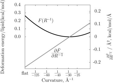
The energy dependence of a single leaflet of DOPE according to the mechanical constants extracted from the x-ray experiment (see, e.g., the literature (1–4)). (Solid line) Free energy; (shaded line) derivative with respect to curvature. The derivative, , is the quantity simulated in this work shown in Fig. 5.
The first method used to determine the spontaneous curvature from simulation computes the deformation energy of a single leaflet present in a lipid bilayer, yielding , the slope of the curve in Fig. 1 at R−1 = 0, which together with an estimate of Kb can be used to reconstruct the curve. Here is the free energy per unit area.
The second method for determining R0 is to simulate the inverse hexagonal phase under various levels of hydration, and calculate the pressure of the water at the interior of the cylinder. In accord with the x-ray experiment, the osmotic pressure Π on the water due to the enclosing lipids will be determined by bending frustration,
| (4) |
with a geometric relation between the surface curvature R−1 and the water volume, Vw.
Although this article emphasizes computing mechanical constants of lipid bilayers, in all cases it is not the spontaneous curvature or bending modulus individually that is directly obtained from a single simulation, but . The usefulness of this quantity may be well beyond parameterization of continuum bilayer models; it is a property of even highly inhomogeneous systems with ambiguous surfaces. Simulations of the inverse hexagonal phase can be executed at various values of R−1, allowing a region of to be fit from the set of values of .
Free energy derivative of planar leaflet curvature
Differentiation of the Helfrich Hamiltonian (per unit area) in Eq. 1 with respect to the curvature, R−1, yields −KbR0−1 (for a planar system). From the Appendix, which contains a review of the theory for computing the bending energy from the lateral pressure profile, pT(z) – pN(z), comes the well-known expression
| (5) |
where pT(z) and pN(z) are the tangential (xy) and normal (z) local pressures for the planar system, respectively. By symmetry, the preferred curvature of a bilayer with the same composition in the upper and lower leaflet is zero. As a practical matter, the limits of integration in Eq. 5 are set to (0, ∞), so that only the upper leaflet is considered. Reversing the sign of z and integrating over the lower leaflet (i.e., with limits (−∞, 0)) provides the same value for the lower leaflet by switching the sense of the curvature. Typically this is written as integrating over the entire bilayer but using the absolute value of z in the integrand. The integration limits are specified here as (−∞, +∞) for use on generic surfaces (in fact the derivation of requires this). The approximation of integrating both halves of the bilayer separately (or with |z| over the entire bilayer) is discussed in the Appendix. The Helfrich energy per unit surface area is
| (6) |
To find the minimum (R0) of Eq. 6 with respect to R−1, the derivative is computed as
| (7) |
where the second term on the right-hand side is evaluated for a planar leaflet. The derivative is zero at R0:
| (8) |
For a pressure profile calculated at zero tension (29), it appears that the pivot at which the spontaneous curvature is computed is arbitrary, as
| (9) |
However, the monolayer bending modulus is measured at an effective pivot point where compression and bending are decoupled, and therefore depends on z0 as described in Kozlov and Winterhalter (37). Equation 7 gives the spontaneous curvature at the pivot at which was measured.
The contribution due to the monolayer bending modulus, could be measured from an experiment, from a power decomposition of simulated bending mode amplitudes for much larger bilayers than are simulated here (33,38,39), or from simulations of the inverse hexagonal phase, as shown below. Alternatively, the monolayer bending modulus can be estimated from the area compressibility and bilayer thickness from polymer brush theory (40,41) or similar analysis (33).
The inverse hexagonal phase
The following analysis of leaflet bending in the inverse hexagonal phase is equivalent to derivations by Gruner et al. (26), and is a simpler case of the general Helfrich shape equation (31). It is repeated here because of the various approximations that are justified to establish its validity, as well to provide a simple framework for analysis of the bending energy if these assumptions break down.
Inverse hexagonal phase lipid simulations are performed at constant isotropic pressure, with periodic boundary conditions, and with the number of molecules fixed. As a result of anisotropic simulation cell deformations, the ratio of the hexagonal cylinder height to diameter is allowed to vary. Before applying the Helfrich model to extract elastic constants, Young-Laplace theory will be applied to relate the pressure at the cylinder interior to the bending energy of the leaflet. The principal assumption is that a cylindrical surface (possibly with finite thickness, as is the case here) encloses a region of fluid with bulk properties, and is itself surrounded by a fluid medium with known pressure. By measuring the pressure difference between the interior and exterior regions as the surface is varied, the force on the surface can be inferred, as these factors balance at equilibrium. The model system has three distinct regions:
-
1.
The interior fluid, assumed to behave like an isotropic fluid under pressure pint with volume Vint;
-
2.
The exterior fluid, which has isotropic pressure pext and volume Vext; and
-
3.
The surface region (of finite thickness), whose boundaries between the other regions are chosen to fulfill the isotropic fluid condition, and which have volume Vsurface.
Under these assumptions there is no surface tension between any of the regions. The possibly complicated free energy of the surface region is parameterized by fs(R,h), where R is the radius of the surface (the choice of which determines the form of fs(R,h)), and h is the simulation cell height. As an example, for an immiscible two-component system, fs(R,h) would be equal to γ2πRh, where γ is the surface tension. The free energy of the entire model system is
| (10) |
Perturbing the model by
| (11) |
changes the surface parameter, R, by ΔR at . To first order in ΔR, the perturbation changes a cylindrical volume from V to V′:
| (12) |
This volume perturbation is the same for all volumes that contain the origin (that is Vtotal and Vint, but not Vext and Vsurface, which have volume changes of zero). Under this deformation, the energy of the surface is perturbed by ΔR∂fs(R, h)/∂R, and the pressure changes account for −Δp(V′ – V) = Δp2πhRΔR, where Δp = pint − pext. For the free energy to be stationary these must sum to zero for infinitesimal perturbations. For the case of an immiscible two-component system with fs(R, h) = 2πhRγ, this results in
| (13) |
which is the Young-Laplace equation for a cylindrical surface subject only to surface tension. For the general case, the stability condition yields
| (14) |
where A is the area of the surface in the simulation cell. The partial derivative indicates that h is held constant; in the following equations a total derivative indicates that variations of R and h are accounted for by keeping a particular quantity fixed, indicated by the subscript outside the parentheses of the derivative. In all cases the free energy of the surface is constrained to be cylindrical, and is in this sense a partial derivative with respect to cylindrical variations of the surface.
Assuming that the interior fluid is incompressible provides a surface equilibrium condition; the surface is allowed to relax subject to the constraint of a constant interior water volume:
| (15) |
However, as will be shown, the Helfrich-bending energy is most conveniently analyzed at constant surface area,
| (16) |
whereas Eq. 14 provides the quantity ∂fs(R, h)/∂R, i.e., the partial derivative at constant h. The situation is reconciled by the geometric relation:
| (17) |
If the surface does not experience any net compression or expansion as it bends, the approximation at left in Eq. 17 will be valid. The same approximation is made for the analysis of planar bending in the Appendix, where it is justified by analyzing geometric parameters of the planar and bent systems. This assumption is also made in the experimental analyses of the inverse hexagonal phase by Rand et al. (1). Combining Eqs. 15–17 yields
| (18) |
and finally
| (19) |
Equation 19 could be used to fit the free energy of bending from a function of any form, for example, if one wishes to include higher-order terms in the expansion of the bending energy.
The position of the surface (i.e., R) is found by determining the pivotal plane where the area is constant as the curvature changes (see Results and Discussion). This choice fixes the computed monolayer bending modulus to be applicable at this point on the leaflet surface and simplifies the resulting model in that the preferred area does not change with curvature. Applying the Helfrich model yields
| (20) |
This is the same result derived in the many experimental works on x-ray diffraction of the inverse hexagonal phase (4,26,43).
Assuming there is sufficient interstitial alkane, and that the tension between the alkane and the lipid tails is negligible, the tension between neighboring simulation cells will be negligible (that is, only fs(R,h) for the leaflet/water surface must be modeled, and not, for example, a γAcell term for the tension between simulation cells). In this case the pressure of the material surrounding the cylinder will be at the simulated external pressure, in this work set to 1 atm. This assumption may be tested in future studies by varying the amount and chain length of the interstitial alkane, as in the experiment in Chen and Rand (5). The framework presented here would be ideal for analyzing this assumption, in that the perturbation in Eq. 11 can be applied to additional terms in Eq. 10. This study will rely on the result of Chen and Rand (5); the monolayer bending modulus and spontaneous curvature do not depend strongly on added alkane levels.
Returning to Eq. 20, it only remains to compute the pressure of the water at the interior of the lipid tube. Although perhaps conceptually simple, the theory for computing the local pressure of even apparently isotropic fluids has been controversial. A method developed by us does exactly that (44), and has been shown to yield accurate pressure differences even for systems with polar/nonpolar interfaces.
A brief comment is necessary to justify the assumption that Δp reflects the constant leaflet surface area ensemble, as some surfaces may somehow be as compressible as they are bendable. Simulated in the NPT ensemble, the cylindrical subsystem can adjust its height and radius constrained by the interior water volume. The analysis concluded with Eq. 20 is based on the assumption that changes in the free energy are due to curvature changes, but it is possible that the area/volume ratio may change due to leaflet compressibility. However, the mechanical constants of compressibility and bending are anticipated to be sufficiently well separated that they can be measured individually. The ratio of effective force constants for free energy changes due to the area compressibility modulus and the monolayer bending modulus is
| (21) |
so that for the curvatures examined herein (roughly 30 Å) the expected ratio for DOPE will be ∼20, and roughly 10 for DOPC. The ensemble is therefore expected to be approximately the constant area ensemble (the modulus measurable by the fluctuations of the area), perturbed slightly by measurable curvature frustration (the curvature frustration measurable by the residual tension). This is analogous to the treatment of the similarity of the pivotal and neutral planes (the neutral plane being the plane for which area and curvature energetics are uncoupled) by Leikin et al. (2).
Details of the calculation of
for various R values of the inverse hexagonal phase are in the following section.
Simulation protocol
The lipid force-field parameters used were from CHARMM C36 (25) with the TIP3P water model standard for recent versions of CHARMM force fields.
All lipid configurations were built using the publicly available CHARMM-GUI web server (45). Inverse hexagonal phase simulations were built starting from oblong rectangles of bilayer with one leaflet removed. The x,z coordinate pair was mapped onto a polar coordinate, rcos(ϕ), with r the target radius of the pivotal plane. Water and tetradecane molecules were then added to approximate the concentrations of the x-ray diffraction work, that is, ∼16% tetradecane. Periodic boundary conditions are applied with hexagonal lattice vectors. The resulting inverse hexagonal phase structures were minimized and subjected to lengthy (∼50–100 ns) equilibration using CHARMM.
Inverse hexagonal phase and water control systems were simulated with NAMD (46). Five simulations with different cylindrical radii (∼27, 29, 30.5, 33.1, and 35 Å) were simulated for ∼250, 150, 120, 120, and 220 ns, respectively (the high and low curvature simulations were extended to improve precision) at 298 K. Each simulation consisted of 125 phospholipids with varying amounts of water (2518, 2769, 3035, 3318, and 3619, respectively). The DOPC inverse hexagonal phase (consisting of 125 phospholipids, 3619 water molecules, with radius ∼33.6 Å) was simulated for 200 ns.
The NAMD simulation protocol used the Langevin thermostat (47) and isotropic Langevin piston barostat (48), suitable for simulations with no kinetic component of interest. The Langevin piston period and decay were set to 200 and 100 fs, respectively. Particle-mesh Ewald (49) (PME) was used for long-ranged electrostatics and van der Waals forces were truncated using the force-switching method of CHARMM between 8 and 12 Å.
Water control simulations necessary to calibrate the internal pressure calculations were also simulated using NAMD, employing the same protocols.
Bilayer pressure profiles were simulated using a development version of the CHARMM simulation package (50) using the methodology described in the literature (28,29,51,52).
To calculate values of at zero curvature (the planar case), the pressure profile of the lipid bilayer is extracted using the Harasima contour, which is uniquely suited to calculations with periodic boundary conditions and PME. The pressure profile was extracted every 100 fs and centered by setting the average of the lipid tail carbons to be z = 0. Equation 7 is evaluated independently for the z > 0 and z < 0 profiles and averaged. Planar systems were equilibrated (>10 ns), then 50-ns production runs were performed at 310 K and at zero tension, so that . Resolution of the normal pressure in the z direction cannot be simply obtained with the Harasima contour and PME electrostatics (52). However, mechanical equilibrium dictates that the normal pressure is evenly distributed through the system. These two conditions (zero tension and uniform normal pressure) are enforced by setting the normal pressure to , and is within standard error (SE) of 1 atm. Enforcing zero tension removes any dependence on the pivot of curvature from Eq. 9.
For the inverse hexagonal phase calculation of , the procedure detailed in Sodt and Pastor (44) is used. Briefly, the pressure of the interior water is evaluated by a mechanical deformation similar to that of Eq. 27, but isolated to only a bulk region of water in the middle, with the rest of the system kept fixed. The free energy of deformation depends on both a contribution from an effective surface tension of the selected region that scales with the change in surface area of the deformation, and a pressure term that scales with the change in volume due to the deformation. A large ensemble is needed to extract a pressure to the required accuracy (anticipated to be on the order of a few atm for DOPE/DOPC). Local pressure calculations for a variety of applied external pressures showed that the ratio of the internal pressure to the effective tension was –0.294 Å−1. The ratio of the internal pressure to the effective tension was constrained to this factor when computing the internal pressure of the hexagonal lipid interiors. The constraint is not absolutely necessary, but does substantially decrease the uncertainty. Recordings of the free energy of deformation were performed every 500 fs and averaged before fitting. In future simulations the frequency of pressure recordings could be increased substantially to reduce error, but the ensemble in this work was generated and postprocessed separately.
Results and Discussion
Fig. 2 shows equilibrated simulation cells of a planar DOPE bilayer (top). Lateral pressure profiles for DOPE and DOPC lipid bilayers are shown in Fig. 3. These profiles of symmetric lipid bilayers should themselves be symmetric. A lack of visual symmetry is due to insufficient sampling. The values of extracted from these profiles have relatively small uncertainties; they do not appear to be sensitive to a fully converged pressure profile.
Figure 2.
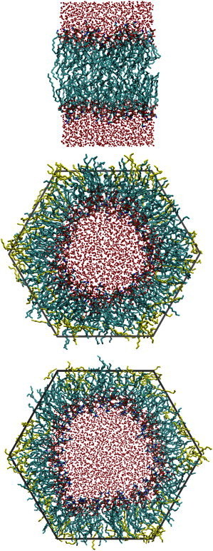
The two phases simulated in this work. (Top) Planar bilayer phase of DOPE. (Middle and bottom) Inverse hexagonal phase renderings of DOPE and DOPC, respectively. (Red spheres) Water molecules (hydrogen atoms not shown). Inverse hexagonal phase: (yellow bars) tetradecane and (dark gray bars) simulation cell boundary. Images were generated using the visualization software VMD.
Figure 3.
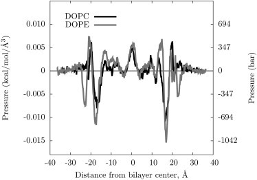
The pressure profiles for DOPC and DOPE bilayers.
As has been discussed in previous studies (29,51), the profile is consistent with the bilayer having a substantial interfacial tension at the surface (characterized by a negative peak where the surface would contract to minimize the polar/apolar exposure) balanced by positive pressure in the middle where the lipid tails are confined. The clearest difference between the DOPE and DOPC profiles is in the headgroup region, as expected. The DOPE lipid has a substantial negative peak at ∼22 Å above the bilayer middle, whereas the DOPC profile is uniformly positive in this region. The DOPE headgroups are smaller and more hydrated than the DOPC headgroups, reflected by a negative peak in the profile where the free energy could be lowered by contraction. The quantity evaluated from Eq. 7 calculated agrees extremely well with the x-ray diffraction measurements, such that when the monolayer bending moduli extracted from the experiment are used, the spontaneous curvature match well (within a few Å for DOPE), as shown in Table 1.
Table 1.
Single leaflet mechanical constants extracted from DOPE and DOPC simulations compared with experiment (3)
| Lipid | Property | Lα (simulation) | HII (simulation) | HII (experiment) |
|---|---|---|---|---|
| DOPE | −0.220 ± 0.001 | −0.43 ± 0.19 | −0.249 | |
| 11.0 ± 4.9 | 6.36 | |||
| R0 | −32.3 ± 1.4 | −25.6 ± 2 | −29.2 | |
| DOPC | −0.085 ± 0.006 | −0.061 | ||
| 0.21 ± 0.03 | 0.098 | |||
| R0 | −65.2 ± 5 | −87.3 |
The quantity (per Å2) has units of kcal/mol/Å, has units of kcal/mol, and R0 has units of Å. The experimental monolayer bending modulus in the table is taken from Fuller and Rand (4), and is measured in the inverse hexagonal phase with tetradecane added. The spontaneous curvature calculated from the planar simulation is based on the experimental monolayer bending modulus.
Fig. 2 also shows the inverse hexagonal phase of DOPE (middle), and the inverse hexagonal phase of DOPC (bottom). In the figure the hexagonal phase of DOPE is at approximately the free energy minimum with respect to curvature frustration. In terms of the Young-Laplace equation, Eq. 13, the tension of the surface is zero, indicating that the pressure is the same on the inside and on the outside (1 atm). For the case of DOPC, the surface is overly curved and would be minimized if flattened; however, in the simulation the water-to-lipid area is naturally fixed and so it exerts a detectable negative pressure on the water.
For the leaflet surface to have well-defined mechanical constants in the Helfrich Hamiltonian model, the surface must have a pivotal plane at which surface bending is not coupled to area compression/expansion (1,53). Moreover, the position of the pivotal plane specifies where the surface is defined and at which the mechanical constants are specified (2,37). The average of the distance from the center of the water region is computed for each unique atom of the lipid molecule, e.g., the phosphorus or nitrogen atom of DOPE. The surface area of that atom type is then computed by 2π〈hr〉, where h is the simulation cell height. The pivotal plane is then defined by the atom whose surface area is constant as a function of bending. At different hydration levels, 〈h〉 and 〈r〉 will adjust; for example, at excess water the height will decrease and the width of the cylinder will expand to keep the area constant at the pivotal plane. Fig. 4 plots the surface areas per lipid for various atom types at the simulated hydration levels, beginning at approximately the headgroup region and extending to the tail. The area is the same at different hydration levels in the vicinity of carbon C22 (see Fig. 4) in the glycerol region, in good agreement with experiment. The area per lipid near the pivotal plane is approximately that of the planar system, ∼65 Å2, indicating the pivotal plane is consistent to planarity.
Figure 4.
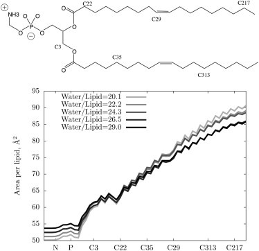
Values of the surface area per lipid measured along the lipid. The pivotal plane is indicated by the area being constant as the surface bends. The area per lipid near the pivotal plane (in the vicinity of carbon C22) is approximately that of the planar system, ∼65 Å2.
Single leaflet mechanical constants extracted from DOPE and DOPC inverse hexagonal phase simulations are shown in Table 1. The data are also plotted in Fig. 5 along with theoretical values derived from the mechanical constants obtained from x-ray diffraction experiments (dashed lines). Multiple simulations of the inverse hexagonal phase of DOPE at different hydration levels calculate and allow for the computation of the bending modulus and spontaneous curvature. The pressure calculation of the inverse hexagonal phase is subject to a substantial amount of noise, and so the uncertainty of the mechanical constants is relatively large; however, the experimental bending modulus and spontaneous curvature are both within ∼1 SE. Extrapolating the to R−1 = 0, the planar case, yields a value that is also within 1 SE of the planar-simulated calculation (in the figure, 1 SD is indicated by the gray-shaded region). This result is significant in that it is a direct indication that the mechanical properties of a planar bilayer can be predicted from a measurement of the curved system, as well as the converse.
Figure 5.
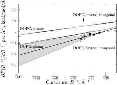
The change of the free energy with curvature, calculated from simulations of a planar bilayer and the inverse hexagonal phase. (Shaded area) One standard-deviation range of the linear fit to the DOPE free energy derivative calculated from the inverse hexagonal phase simulation. (Dashed lines) X-ray diffraction results for inverse hexagonal phase systems (DOPC upper; DOPE lower).
For DOPC, only a single inverse hexagonal phase simulation was performed, so mechanical constants can only be inferred when coupled with the experimental information. The negative pressure at the middle of the DOPC inverse hexagonal phase indicates that the lipid bilayer is acting to expand the water region, a result consistent with a flatter preferred curvature for DOPC. A caveat of this calculation is that the DOPC inverse hexagonal phase appears to have kinks or other defects; its curvature is not uniform like that of DOPE, as illustrated in Fig. 2 (bottom).
Conclusions
This article presented two techniques for calculating the derivative of the free energy with respect to bilayer leaflet bending, . The first method, for planar systems, relied on the single leaflet lateral pressure profile from the bilayer simulation. The second method, analogous to the x-ray diffraction experiment used to measure curvature properties, computes the pressure at the center of the inverse hexagonal phase. The two methods were shown to produce consistent results, indicating that the mechanical properties of planar systems can be extrapolated from curved measurements (as well as the converse).
This study serves as a partial validation of the CHARMM C36 force field for simulating the inverse hexagonal phase. The presence of a well-defined pivotal plane with an area per lipid consistent with the planar phase, as well as accurate and consistent mechanical properties, demonstrates that the force-field parameters are transferable to high curvature.
The defects present in the DOPC inverse hexagonal phase simulation suggest that the calculated is an underestimate, in that the curvature frustration would be partially relieved by the defects. This is not reflected in the value of the interior pressure; i.e., the simulation indicates a substantial negative pressure at the water interior. It is possible that in the future the technique presented herein, combined with the Helfrich model, could be used to predict the free energy cost of the defects by analyzing their frequency and effect on the osmotic pressure, although more data would be required to achieve the level of precision required.
It is anticipated that the simulation technique presented in this work can be used to calculate for surfaces with biologically active molecules embedded, isolating their contribution to bilayer mechanics. Additionally, the effect of surface curvature on the conformational state and orientation of, e.g., peptides may be deduced by embedding them in these highly curved surfaces (similar to a recent experiment by Tristram-Nagle et al. (54)).
Acknowledgments
The authors thank the editor, Reinhard Lipowsky, and an anonymous reviewer for providing comments that substantially improved the work. Additionally, we thank Bernard Brooks for helpful discussions. NAMD was developed by the Theoretical and Computational Biophysics Group in the Beckman Institute for Advanced Science and Technology at the University of Illinois at Urbana-Champaign.
This work was supported by the Intramural Research Program of the National Institutes of Health, National Heart, Lung and Blood Institute.
Appendix: Free Energy Derivative of Planar Leaflet Curvature
The following derivation gives the same result as Szleifer et al. (27), which examines the detailed origins of stress and curvature strain in lipid bilayers and monolayers, and has been used in recent literature to calculate the spontaneous curvature (11–14). Here it is based on the statistical mechanical first-order change in the free energy of an ensemble from Schofield and Henderson (28). This derivation provides the free energy derivative without explicitly invoking a continuum model of the bilayer. That is, the derivative is valid whether a continuum representation is valid or not. However, interpreting the derivative as implying mechanical constants does require the definition and validity of a continuum model.
For a simulation of a flat system, will be computed by a mechanical theory of deformations that requires a local pressure (strain) p(r) and displacement field u(r). As shown by Schofield and Henderson (28), the free energy to first order in the mechanical deformation u(r) is calculated according to
| (22) |
where u(r) transforms the coordinates of the equilibrium ensemble . The second term is the expectation value of how the displacement acts on the internal forces of the ensemble, and the first term is the change in free energy from kinetic energy due to expansion or contraction of a region (note that is the Jacobian factor, the derivative of the α-Cartesian component of u(r) with respect to Cartesian component α). The ensemble average is often transformed into a spatially resolved representation of the stress on which a generic strain u(r) can act,
| (23) |
so that after integration by parts, the gradient in ∇βpαβ(r) is transferred to u(r) and
| (24) |
where C0i is a contour connecting some fixed arbitrary point to ri; uαβ (r) is the derivative with respect to Cartesian component β of the α-component of u(r); pαβ(r) is the local pressure tensor (that is, the β-component of the force acting along direction α of a material at r); and ∇f(r) = 0. Equation 24 is attractive because pαβ can be constructed to behave like one would expect a local pressure to behave (depending on the choice of C0i), e.g., having a negative value where a subsystem appears to be pulled upon, like an extended spring, or having zero stress where locally a system behaves like a pure fluid. However, experimentally observable quantities may be calculated from Eq. 22 just as rigorously as Eq. 24 and so do not depend on C0i.
As shown by Schofield and Henderson (28), various physical quantities can be calculated from Eq. 22 (if ΔF is calculated on-the-fly) or Eq. 24 (if pαβ is postprocessed) when the system is constrained by an external mechanism, for example, the total pressure when the displacement u(r) is proportional to r (that is, an isotropic expansion/compression). A specific transformation uα (r) for curving will be used to calculate the free energy of deformation of a surface constrained to be flat by periodic boundary conditions.
Given a segment of a flat system (shown schematically as a rectangle in Fig. 6), a volume-conserving deformation can be constructed to yield a new system with curvature R−1. The original coordinates, (x, z), are transformed into the new coordinates, (x′, z′), by a transformation that creates a radius R and fixed arc at z = 0 and a radius of R1 (with center at z = −R) at z′. The value R1 is defined such that the area of the transformed rectangle is preserved:
| (25) |
From this follows the transformed coordinates:
| (26) |
Figure 6.
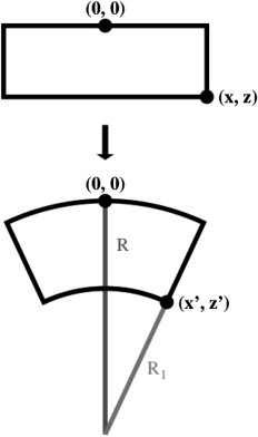
The coordinate transformation [(x, z) to (x′, z′)] that causes a curvature-inducing mechanical deformation. The deformation is a virtual transformation in that the ensemble is not actually moved, but rather the free energy derivative is measured along the transformation.
The bilayer is laterally translationally invariant, so the bending free energy can be calculated per lateral unit distance, and the new coordinates can be expanded within the vicinity of x = 0. To linear in R−1, we have
| (27) |
yielding the transformation
where x and z are the Cartesian components of r. Inserting the transformation in Eq. 27 into Eq. 24 yields in Eq. 5.
Verification of volume-conserving bending is possible by comparing the structure of the planar bilayer with the curved inverse hexagonal phase. The average height zi (for the planar bilayer) and radius ri (for the inverse hexagonal phases) of each atom type i is recorded. The atom i approximately corresponding to the pivotal plane is selected based on area-conservation (atom C31 in the CHARMM force field), as shown in Fig. 4. The volume of material between the surface defined by the average position of atom i and the pivotal plane atom (pp) is
| (28) |
| (29) |
where NL is the number of lipids in the planar bilayer and AL is the average area per lipid. By definition at the pivotal plane, 2πhrpp/NL = AL. Inserting this into Eq. 28 and equating the two volumes (which would imply volume conservation during bending) yields
| (30) |
These quantities are computed directly from the saved trajectories of the simulations. A least-squares fit of y = kx to the left side of Eq. 30 against the right gives a slope k of 1.06, with coefficient of determination equal to 0.995. This indicates that the volume is conserved at high curvature. The assumption of volume conservation is likely even more accurate at low curvature, although this would require an infeasibly large simulation to test. The deviation from volume-conservation increases further from the pivotal plane, that is, where tetradecane begins filling the tail space, and where the headgroup dehydrates.
Equation 22 is valid if the system forces (excluding external forces) are all contained in the volume of integration, V. The first part of this work involving the planar system relies on an assumption requiring validation: That the local pressure in half of the bilayer simulation cell (containing one leaflet) represents, with sufficient fidelity, the case of a single leaflet with an infinite water slab above, and an infinite alkane region below (such that there are no tensions between the layer and the surroundings). The Harasima contour (55) used in this work for calculating pαβ(r) is valid in the water region because the local tension goes to zero in this area, as can be seen in Fig. 3. The commonly used Irving-Kirkwood (56) contour also has this property, but is not feasible with long-range Coulomb interactions (52). For the alkyl tail region, the validity is not as clear because the bilayer middle is not necessarily tensionless. However, the accuracy of the calculated indicates that this approximation is a good one.
References
- 1.Rand R.P., Fuller N.L., Parsegian V.A. Membrane curvature, lipid segregation, and structural transitions for phospholipids under dual-solvent stress. Biochemistry. 1990;29:76–87. doi: 10.1021/bi00453a010. [DOI] [PubMed] [Google Scholar]
- 2.Leikin S., Kozlov M.M., Rand R.P. Measured effects of diacylglycerol on structural and elastic properties of phospholipid membranes. Biophys. J. 1996;71:2623–2632. doi: 10.1016/S0006-3495(96)79454-7. [DOI] [PMC free article] [PubMed] [Google Scholar]
- 3.Chen Z., Rand R.P. The influence of cholesterol on phospholipid membrane curvature and bending elasticity. Biophys. J. 1997;73:267–276. doi: 10.1016/S0006-3495(97)78067-6. [DOI] [PMC free article] [PubMed] [Google Scholar]
- 4.Fuller N., Rand R.P. The influence of lysolipids on the spontaneous curvature and bending elasticity of phospholipid membranes. Biophys. J. 2001;81:243–254. doi: 10.1016/S0006-3495(01)75695-0. [DOI] [PMC free article] [PubMed] [Google Scholar]
- 5.Chen Z., Rand R.P. Comparative study of the effects of several n-alkanes on phospholipid hexagonal phases. Biophys. J. 1998;74:944–952. doi: 10.1016/S0006-3495(98)74017-2. [DOI] [PMC free article] [PubMed] [Google Scholar]
- 6.Lundbaek J.A., Maer A.M., Andersen O.S. Lipid bilayer electrostatic energy, curvature stress, and assembly of gramicidin channels. Biochemistry. 1997;36:5695–5701. doi: 10.1021/bi9619841. [DOI] [PubMed] [Google Scholar]
- 7.Botelho A.V., Huber T., Brown M.F. Curvature and hydrophobic forces drive oligomerization and modulate activity of rhodopsin in membranes. Biophys. J. 2006;91:4464–4477. doi: 10.1529/biophysj.106.082776. [DOI] [PMC free article] [PubMed] [Google Scholar]
- 8.Ramamurthi K.S., Losick R. Negative membrane curvature as a cue for subcellular localization of a bacterial protein. Proc. Natl. Acad. Sci. USA. 2009;106:13541–13545. doi: 10.1073/pnas.0906851106. [DOI] [PMC free article] [PubMed] [Google Scholar]
- 9.Kozlovsky Y., Chernomordik L.V., Kozlov M.M. Lipid intermediates in membrane fusion: formation, structure, and decay of hemifusion diaphragm. Biophys. J. 2002;83:2634–2651. doi: 10.1016/S0006-3495(02)75274-0. [DOI] [PMC free article] [PubMed] [Google Scholar]
- 10.Anitei M., Hoflack B. Bridging membrane and cytoskeleton dynamics in the secretory and endocytic pathways. Nat. Cell Biol. 2012;14:11–19. doi: 10.1038/ncb2409. [DOI] [PubMed] [Google Scholar]
- 11.Marrink S.J., Risselada H.J., de Vries A.H. The MARTINI force field: coarse grained model for biomolecular simulations. J. Phys. Chem. B. 2007;111:7812–7824. doi: 10.1021/jp071097f. [DOI] [PubMed] [Google Scholar]
- 12.Orsi M., Haubertin D.Y., Essex J.W. A quantitative coarse-grain model for lipid bilayers. J. Phys. Chem. B. 2008;112:802–815. doi: 10.1021/jp076139e. [DOI] [PubMed] [Google Scholar]
- 13.Samuli Ollila O.H., Róg T., Vattulainen I. Role of sterol type on lateral pressure profiles of lipid membranes affecting membrane protein functionality: comparison between cholesterol, desmosterol, 7-dehydrocholesterol and ketosterol. J. Struct. Biol. 2007;159:311–323. doi: 10.1016/j.jsb.2007.01.012. [DOI] [PubMed] [Google Scholar]
- 14.Ollila S., Hyvönen M.T., Vattulainen I. Polyunsaturation in lipid membranes: dynamic properties and lateral pressure profiles. J. Phys. Chem. B. 2007;111:3139–3150. doi: 10.1021/jp065424f. [DOI] [PubMed] [Google Scholar]
- 15.Ollila O.H.S., Vattulainen I. Lateral pressure profiles in lipid membranes: dependence on molecular composition. In: Sansom M.S.P., Biggin P.C., editors. Molecular Simulations and Biomembranes. Royal Society of Chemistry; London, United Kingdom: 2010. pp. 27–56. [Google Scholar]
- 16.Wang Z.-J., Deserno M. A systematically coarse-grained solvent-free model for quantitative phospholipid bilayer simulations. J. Phys. Chem. B. 2010;114:11207–11220. doi: 10.1021/jp102543j. [DOI] [PMC free article] [PubMed] [Google Scholar]
- 17.Orsi M., Essex J.W. The ELBA force field for coarse-grain modeling of lipid membranes. PLoS ONE. 2011;6:e28637. doi: 10.1371/journal.pone.0028637. [DOI] [PMC free article] [PubMed] [Google Scholar]
- 18.Gullingsrud J., Schulten K. Lipid bilayer pressure profiles and mechanosensitive channel gating. Biophys. J. 2004;86:3496–3509. doi: 10.1529/biophysj.103.034322. [DOI] [PMC free article] [PubMed] [Google Scholar]
- 19.Cantor R.S. The influence of membrane lateral pressures on simple geometric models of protein conformational equilibria. Chem. Phys. Lipids. 1999;101:45–56. doi: 10.1016/s0009-3084(99)00054-7. [DOI] [PubMed] [Google Scholar]
- 20.Xing C., Ollila S., Faller R. Asymmetric nature of lateral pressure profiles in supported lipid membranes and its implications for membrane protein functions. Soft Matter. 2009;5:3258–3261. [Google Scholar]
- 21.Baoukina S., Marrink S.J., Tieleman D.P. Lateral pressure profiles in lipid monolayers. Faraday Discuss. 2010;144:393–409. doi: 10.1039/b905647e. discussion 445–481. [DOI] [PubMed] [Google Scholar]
- 22.Vanegas J.M., Longo M.L., Faller R. Crystalline, ordered and disordered lipid membranes: convergence of stress profiles due to ergosterol. J. Am. Chem. Soc. 2011;133:3720–3723. doi: 10.1021/ja110327r. [DOI] [PubMed] [Google Scholar]
- 23.Risselada H.J., Marrink S.J. Curvature effects on lipid packing and dynamics in liposomes revealed by coarse grained molecular dynamics simulations. Phys. Chem. Chem. Phys. 2009;11:2056–2067. doi: 10.1039/b818782g. [DOI] [PubMed] [Google Scholar]
- 24.Cooke I.R., Deserno M. Coupling between lipid shape and membrane curvature. Biophys. J. 2006;91:487–495. doi: 10.1529/biophysj.105.078683. [DOI] [PMC free article] [PubMed] [Google Scholar]
- 25.Klauda J.B., Venable R.M., Pastor R.W. Update of the CHARMM all-atom additive force field for lipids: validation on six lipid types. J. Phys. Chem. B. 2010;114:7830–7843. doi: 10.1021/jp101759q. [DOI] [PMC free article] [PubMed] [Google Scholar]
- 26.Gruner S.M., Parsegian V.A., Rand R.P. Directly measured deformation energy of phospholipid HII hexagonal phases. Faraday Discuss. Chem. Soc. 1986;81:29–37. doi: 10.1039/dc9868100029. [DOI] [PubMed] [Google Scholar]
- 27.Szleifer I., Kramer D., Safran S.A. Molecular theory of curvature elasticity in surfactant films. J. Chem. Phys. 1990;92:6800–6817. [Google Scholar]
- 28.Schofield P., Henderson J.R. Statistical mechanics of inhomogeneous fluids. Proc. R. Soc. Lond. A Math. Phys. Sci. 1982;379:231–246. [Google Scholar]
- 29.Goetz R., Lipowsky R. Computer simulations of bilayer membranes: self-assembly and interfacial tension. J. Chem. Phys. 1998;108:7397–7409. [Google Scholar]
- 30.Helfrich W. Elastic properties of lipid bilayers: theory and possible experiments. Z. Naturforsch. C. 1973;28:693–703. doi: 10.1515/znc-1973-11-1209. [DOI] [PubMed] [Google Scholar]
- 31.Zhong-can O.-Y., Helfrich W. Instability and deformation of a spherical vesicle by pressure. Phys. Rev. Lett. 1987;59:2486–2488. doi: 10.1103/PhysRevLett.59.2486. [DOI] [PubMed] [Google Scholar]
- 32.Marsh D. Lateral pressure profile, spontaneous curvature frustration, and the incorporation and conformation of proteins in membranes. Biophys. J. 2007;93:3884–3899. doi: 10.1529/biophysj.107.107938. [DOI] [PMC free article] [PubMed] [Google Scholar]
- 33.Goetz R., Gompper G., Lipowsky R. Mobility and elasticity of self-assembled membranes. Phys. Rev. Lett. 1999;82:221–224. [Google Scholar]
- 34.Gawrisch K., Parsegian V.A., Rand R.P. Energetics of a hexagonal-lamellar-hexagonal-phase transition sequence in dioleoylphosphatidylethanolamine membranes. Biochemistry. 1992;31:2856–2864. doi: 10.1021/bi00126a003. [DOI] [PubMed] [Google Scholar]
- 35.Siegel D.P., Kozlov M.M. The Gaussian curvature elastic modulus of n-monomethylated dioleoylphosphatidylethanolamine: relevance to membrane fusion and lipid phase behavior. Biophys. J. 2004;87:366–374. doi: 10.1529/biophysj.104.040782. [DOI] [PMC free article] [PubMed] [Google Scholar]
- 36.Siegel D.P. The Gaussian curvature elastic energy of intermediates in membrane fusion. Biophys. J. 2008;95:5200–5215. doi: 10.1529/biophysj.108.140152. [DOI] [PMC free article] [PubMed] [Google Scholar]
- 37.Kozlov M.M., Winterhalter M. Elastic moduli for strongly curved monolayers. Position of the neutral surface. J. Phys. II. (Fr.) 1991;1:1077–1084. [Google Scholar]
- 38.Lindahl E., Edholm O. Mesoscopic undulations and thickness fluctuations in lipid bilayers from molecular dynamics simulations. Biophys. J. 2000;79:426–433. doi: 10.1016/S0006-3495(00)76304-1. [DOI] [PMC free article] [PubMed] [Google Scholar]
- 39.Watson M.C., Brown F.L.H. Interpreting membrane scattering experiments at the mesoscale: the contribution of dissipation within the bilayer. Biophys. J. 2010;98:L9–L11. doi: 10.1016/j.bpj.2009.11.026. [DOI] [PMC free article] [PubMed] [Google Scholar]
- 40.Rawicz W., Olbrich K.C., Evans E. Effect of chain length and unsaturation on elasticity of lipid bilayers. Biophys. J. 2000;79:328–339. doi: 10.1016/S0006-3495(00)76295-3. [DOI] [PMC free article] [PubMed] [Google Scholar]
- 41.Pan J., Tristram-Nagle S., Nagle J.F. Temperature dependence of structure, bending rigidity, and bilayer interactions of dioleoylphosphatidylcholine bilayers. Biophys. J. 2008;94:117–124. doi: 10.1529/biophysj.107.115691. [DOI] [PMC free article] [PubMed] [Google Scholar]
- 42.Reference deleted in proof.
- 43.Kirk G.L., Gruner S.M., Stein D.L. A thermodynamic model of the lamellar to inverse hexagonal phase transition of lipid membrane-water systems. Biochemistry. 1984;23:1093–1102. [Google Scholar]
- 44.Sodt A.J., Pastor R.W. The tension of a curved surface from simulation. J. Chem. Phys. 2012;137:234101. doi: 10.1063/1.4769880. [DOI] [PMC free article] [PubMed] [Google Scholar]
- 45.Jo S., Kim T., Im W. CHARMM-GUI: a web-based graphical user interface for CHARMM. J. Comput. Chem. 2008;29:1859–1865. doi: 10.1002/jcc.20945. [DOI] [PubMed] [Google Scholar]
- 46.Phillips J.C., Braun R., Schulten K. Scalable molecular dynamics with NAMD. J. Comput. Chem. 2005;26:1781–1802. doi: 10.1002/jcc.20289. [DOI] [PMC free article] [PubMed] [Google Scholar]
- 47.Martyna G.J., Tobias D.J., Klein M.L. Constant pressure molecular dynamics algorithms. J. Chem. Phys. 1994;101:4177–4189. [Google Scholar]
- 48.Feller S.E., Zhang Y., Brooks B.R. Constant pressure molecular dynamics simulation: the Langevin piston method. J. Chem. Phys. 1995;103:4613–4621. [Google Scholar]
- 49.Darden T., York D., Pedersen L. Particle mesh Ewald: an Nlog(N) method for Ewald sums in large systems. J. Chem. Phys. 1993;98:10089–10092. [Google Scholar]
- 50.Brooks B.R., Brooks C.L., 3rd, Karplus M. CHARMM: the biomolecular simulation program. J. Comput. Chem. 2009;30:1545–1614. doi: 10.1002/jcc.21287. [DOI] [PMC free article] [PubMed] [Google Scholar]
- 51.Lindahl E., Edholm O. Spatial and energetic-entropic decomposition of surface tension in lipid bilayers from molecular dynamics simulations. J. Chem. Phys. 2000;113:3882–3893. [Google Scholar]
- 52.Sonne J., Hansen F.Y., Peters G.H. Methodological problems in pressure profile calculations for lipid bilayers. J. Chem. Phys. 2005;122:124903. doi: 10.1063/1.1862624. [DOI] [PubMed] [Google Scholar]
- 53.Marsh D. Pivotal surfaces in inverse hexagonal and cubic phases of phospholipids and glycolipids. Chem. Phys. Lipids. 2011;164:177–183. doi: 10.1016/j.chemphyslip.2010.12.010. [DOI] [PubMed] [Google Scholar]
- 54.Tristram-Nagle S., Chan R., Nagle J.F. HIV fusion peptide penetrates, disorders, and softens T-cell membrane mimics. J. Mol. Biol. 2010;402:139–153. doi: 10.1016/j.jmb.2010.07.026. [DOI] [PMC free article] [PubMed] [Google Scholar]
- 55.Harasima A. Molecular theory of surface tension. Adv. Chem. Phys. 1958;1:203–237. [Google Scholar]
- 56.Irving J.H., Kirkwood J.G. The statistical mechanical theory of transport processes. IV. The equations of hydrodynamics. J. Chem. Phys. 1950;18:817–829. [Google Scholar]