

Abstract
In this paper, we propose a particle filtering approach for the problem of registering two point sets that differ by a rigid body transformation. Typically, registration algorithms compute the transformation parameters by maximizing a metric given an estimate of the correspondence between points across the two sets of interest. This can be viewed as a posterior estimation problem, in which the corresponding distribution can naturally be estimated using a particle filter. In this work, we treat motion as a local variation in pose parameters obtained by running a few iterations of a certain local optimizer. Employing this idea, we introduce stochastic motion dynamics to widen the narrow band of convergence often found in local optimizer approaches for registration. Thus, the novelty of our method is threefold: First, we employ a particle filtering scheme to drive the point set registration process. Second, we present a local optimizer that is motivated by the correlation measure. Third, we increase the robustness of the registration performance by introducing a dynamic model of uncertainty for the transformation parameters. In contrast with other techniques, our approach requires no annealing schedule, which results in a reduction in computational complexity (with respect to particle size) as well as maintains the temporal coherency of the state (no loss of information). Also unlike some alternative approaches for point set registration, we make no geometric assumptions on the two data sets. Experimental results are provided that demonstrate the robustness of the algorithm to initialization, noise, missing structures, and/or differing point densities in each set, on several challenging 2D and 3D registration scenarios.
Index Terms: Point set registration, particle filters, pose estimation
1 Introduction
A well-studied problem in computer vision is the fundamental task of optimally aligning two point clouds. This has numerous applications, ranging from medical image analysis, quality control, military surveillance, and tracking; see [15], [3], [4], [9], [22] and the references therein. In general, point set registration is a two part problem: First, the correspondences between points across the two sets of interest must be established, and then the transformation parameters are estimated. In this work, we approach the coupled task as a posterior estimation problem, in which we draw upon filtering principles to estimate the corresponding distribution via a particle filter (PF). However, to appreciate the contributions presented in this note, we first recall some of the key results that have been made pertaining to the field of point set registration.
By decoupling the problem of estimating correspondences and the transformation parameters, Besl and McKay [3] introduce the well-known Iterative Closest Point (ICP) algorithm. Given an initial alignment, ICP assigns a set of correspondences based on the L2 distance, computes the transformation parameters, and then proceeds in an iterative manner with a newly updated set of correspondences. However, the basic approach is widely known to be susceptible to local minima. To address this issue, Fitzgibbon [10] introduces a robust variant by optimizing the cost function with the Levenberg-Marquardt algorithm. Even though this method and variants of ICP [4], [10] do improve the narrow band of convergence, they are still heavily dependent on the initial alignment and may fail due to the existence of homologies (due to noise, clutter, outliers) within the correspondence matrix. For instance, Fig. 1 demonstrates a common problem in registration in which a poor initial alignment can yield an incorrect registration to the “wrong” side of the truck.
Fig. 1.

Common problems in point set registration. (a) Initial alignment that can yield an incorrect registration to the “wrong” side of the truck when using iterative-based techniques. (b) Dense point set. (c) Sparse point set.
To overcome the problem of sensitivity to initialization, a second class of point set registration schemes, referred to as “shape descriptors,” has emerged in the graphics community [11], [20], [16]. Typically, these approaches introduce structural information into the registration scheme. This allows them to perform well under poor initializations as well as to handle partial structures or missing information. Unfortunately, these techniques are generally ill suited for tasks such as tactical tracking, whereby the point set density is unknown and can be adjusted during the acquisition phase. Without special consideration, registration may fail if one tries to match a sparse cloud to a dense cloud. See Fig. 1 for an illustration of “sparsity.”
Another proposed methodology for solving the problem of dependency on initial alignment (as seen standard in ICP and other iterative-based methods) is the Robust Point Matching (RPM) algorithm [6], [5]. This approach performs an exhaustive search that is reduced over time with an appropriate annealing schedule. However, Sofka et al. [30] demonstrate the failure of RPM in the presence of clutter or when certain structures are missing.
The use of robust statistics and measures form the next class of point set registration algorithms [17], [31]. Specifically, representing point sets as probability densities, Tsin and Kanade [32] propose a Kernel Correlation (KC) approach using kernel density estimates. The method computes the optimal alignment by reducing the “distance” between sets via a similarity metric. An extension is considered in [19] through the use of a Gaussian mixture model. In particular, both of these approaches propose a registration technique without explicitly establishing point correspondences between data sets, and can be considered as multiply-linked ICP registration schemes. While this allows for a wider basin of convergence than traditional ICP-like algorithms, it can be readily seen that the approaches become computationally expensive as one point set must interact with each point in the opposing set. Moreover and more importantly, to overcome poor initializations or missing information, the KC algorithm must use a kernel with a larger bandwidth. This effectively “smoothes” the data sets, and results in an alignment of distributions spatially. Hence, there is a trade-off between the pointwise accuracy (increases with smaller bandwidth) and its dependency on initial alignment or missing information (decreases with larger bandwidth).
Consequently, a natural extension would be to employ a multiscale approach as proposed by Granger and Pennec [14]. Their algorithm begins by aligning the center of mass of each point set, and then proceeds with the lowering of a “smoothing” factor to ensure the pointwise accurate feature of ICP. We should note that the framework presented in this paper shares certain similarities with this method; notably, the general notion of having a global-to-local approach as well as invoking a robust objective functional through the use of Gaussian mixture model. However, while [32], [19] can be reinterpreted as a multiply-linked ICP registration scheme, our proposed algorithm can be considered as a switching stochastic ICP approach where one point set interacts only with a handful of correspondences. Thus, we keep the explicit establishment of point correspondences as in the iterative techniques, which ensures, on the local level, an accurate ICP-like algorithm. Moreover, we do not require an annealing schedule in our global-to-local approach such as that proposed in [14] since this is naturally embedded in the diffusion process of the prediction model. In Section 5, we compare the KC algorithm with the particle filtering technique discussed in this present work.
Related results that follow the approach presented in this paper are based on filtering methods [23], [24], [26], [21]. Ma and Ellis [23] pioneered the use of the Unscented Particle Filter (UPF) for point set registration. Although the algorithm accurately registers small data sets, it requires a large number of particles (5,000) to perform accurate registration. Because of the large computational costs involved using large sample sizes, the method becomes impractical for large data sets. To address this issue, Moghari and Abolmaesumi [26] propose using an Unscented Kalman Filter (UKF) approach. However, their method suffers the limitation of assuming a unimodal probability distribution of the state vector, and thus may fail for multimodal distributions.
It is important to note that, although the schemes mentioned above are based on filtering principles, the overall framework and algorithm proposed in this work is very different. In [23], [24], Ma and Ellis and, in [26], Moghari and Abolmaesumi employ the closest point operator in the posterior for online estimation of the pose parameters. The operation itself is defined by the L2 distance, which is known to be susceptible to noise and outliers. In this work, we invoke a novel robust local optimizer within the observation model. This enables us to define “motion” or uncertainty in the registration process as local variations in the pose parameters. In doing so, we then propose a prediction model that stochastically diffuses particles in the direction of uncertainty of the transformation. Moreover, both [24], [26] use a deterministic annealing schedule to drive their prediction model. Even though the estimates are improved over time and the variance of particles is reduced, the annealing schedule itself does not incorporate any information learned online. Instead, the parameters of the annealing schedule are chosen a priori. By incorporating information that is learned online through the diffusion process, our proposed technique requires no annealing schedule. Altogether, this confers a high level of robustness to noise, extraneous structures, and initialization, while still maintaining both the temporal coherency of the state and a pointwise accurate scheme throughout the registration process.
Thus, our contributions in this paper are threefold. First, we employ a particle filtering approach with a nonparametric prediction model to drive the point set registration process. Second, we derive an approximation for the correlation measure for two point sets formed by a mixture of Gaussian. From this, we present an iterative-based local optimizer that can be reinterpreted as a robust version of ICP. Last, to increase the robustness of the registration performance, we invoke this optimizer by introducing a dynamical model of uncertainty for the transformation parameters. We should also note that there is a conference version of this work [29].
The remainder of the paper is organized as follows: In the next section, we discuss the particle filter and derive a novel local optimizer. In Section 3, we describe the registration algorithm along with the specifics of the prediction step, measurement model, and the resampling scheme. Section 4 provides numerical implementation details. Experimental results are given in Section 5. Finally, we discuss future work in Section 6.
2 Preliminaries
In this section, we derive a local optimizer for point set registration as well review some basic notions from the theory of particle filtering, which we will need in the sequel.
2.1 The Objective Functional
We now formulate and derive a novel local optimizer that is based on the correlation measure for point set registration. Specifically, we form an approximation for two sets of data described by mixture of Gaussian, and then show that the resulting registration scheme is a robust variant of ICP. We should note that, although similarities exist with those of [32], [19], a key difference is that we keep explicit point correspondences. That is, rather than smoothing point sets in a constant or multiscale fashion, we later employ this optimizer in the measurement functional as the “local” component in an otherwise “global” scheme.
2.1.1 An Approximation of the Correlation Measure for a Mixture of Gaussians
In what follows, we have assumed that we are given two mixtures of Gaussian distributions. We denote these distributions m(y) and d(y) as model and data, respectively. Specifically, they have the form and , where μ and Σ are the mean vector and covariance matrix of each mixture component, respectively.
Let us now assume that it is possible to obtain a closed-form expression for the correlation measure between these two mixtures of distributions, and that the modes of each of the neighboring mixtures are far apart. In other words, as in [12], it is sufficient to consider only a component of a mixture in evaluating m(y) or d(y). We note that, although this assumption is generally valid for point sets, it may not be for other applications. Nevertheless, it can be seen that one appropriate approximation of the correlation measure is to match a single component of m(y) to each component of d(y), that is,
Given the above assumptions, the term αjφmj (y | μmj, Σmj), which is in the same proximity of the component βi · φdi (y | μdi, Σdi), dominates the integral ∫ βiφdi (y | μdi, Σdi) · m(y)dy. Now the term maxj(·) above is realizable by computing the following:
| (1) |
where and correspond to the component that is the minimum euclidean distance for the ith component in the mixture modeled by d(y).
2.1.2 Local Optimizer for Point Set Registration
Suppose now that we are given two point sets that lie in IRn. Previously denoted as model and data, we can further describe each finite point sets by their respective elements and . That is, each point within their respective point clouds forms a Gaussian distribution, whereby the mean vector is the location of a point and the covariance is the identity matrix, e.g., μmi = mi, Σmi = I. Assuming a rigid body transformation, T(d⃗, θ) : IRn ↦ IRn, for a set data points d⃗i and model points m⃗j, we seek to find a rotational matrix R and a translation vector t that minimizes the following energy functional:
| (2) |
Similarly to that of [19], we are now able to employ the following formula: ∫ φ1(y | μ1, Σ1) φ2(y | μ2, Σ2) = φ(0 | μ1 − μ2, Σ1 + Σ2). Thus,
| (3) |
where and
Moreover, if we can obtain the surface normals of the model set, we can then further increase the robustness of the optimizer. This is done by dotting (3) with the (outward) surface unit normal n⃗ of the corresponding model point. The resulting expression that is to be optimized is now given as
| (4) |
where is the corresponding outward surface unit normal associated with model point . Typically, a correspondence matrix C is used to relate the associated model point mj to the data point di. After establishing these point correspondences, the optimal transformation, φ = {t⃗, R}, can be computed with the minimization of (4).
For the derivation of minimizing (4), the interested reader may refer to the Appendix. It is important to note though that, after the transformation parameters are computed, a new “image” of the correspondence matrix is formed by applying the transformation T(d⃗, φ). The algorithm proceeds in an iterative manner until convergence or a stopping criterion is reached.
As compared to the methodology proposed in [32], [19], we have explicitly kept the point-to-point correspondences. Moreover, by keeping this explicit representation, we are then able to incorporate surface normals. The resulting optimizer can be seen as a robust variant of ICP whereby we penalize outliers through the exponential term. Thus, we refer to this as a “local” optimizer in the sense of its narrow band of convergence. However, when used in conjunction with a particle filter, the basin of convergence is significantly widened. We also note that other optimizers [4], [10], [15] may be considered instead of the proposed functional presented here.
2.2 Particle Filtering
We now briefly revisit the basic notions and the generic setup of particle filtering as well as its motivation in point set registration.
2.2.1 Background and Generic Scheme
Letting x ∈ IRn, Monte Carlo methods allow for the evaluation of a multidimensional integral I = ∫ g(x)dx via a factorization of the form I = f(x)π(x)dx, whereby π(x) can be interpreted as a probability distribution. Taking samples from such a distribution in the limit yields the estimate of I that would otherwise be difficult or impossible to compute. However, generating samples from the posterior distribution is usually not possible. Thus, if one can only generate samples from a similar density q(x), the problem becomes one of “importance sampling.” That is, the Monte Carlo estimate of I can be computed by generating N ≫ 1 independent samples {xi; i = 1, …, N} distributed according to q(x) by forming the weighted sum: , where represents the normalized importance weight. Consequently, by employing Monte Carlo methods in conjunction with Bayesian filtering, Gordon et al. [13] first introduced the PF. We refer the reader to [28], [8] for an in-depth discussion on Monte Carlo methods and particle filtering schemes.
Now considering xt ∈ IRn to be a state vector, with zt ∈ IRn being its corresponding measurement, particle filtering is a technique for implementing a recursive Bayesian filter through Monte Carlo simulations. At each time t, a cloud of N particles is produced, , whose empirical measure closely “follows” p(xt | z0:t) = πt(xt | z0:t), the posterior distribution of the state given the past observations, z0:t.
The algorithm starts with sampling N times from the initial state distribution π0(x0) in order to approximate it by , and then implements Bayesian recursion at each step. With the above formulation, the distribution of the state at t −1 is given by . The algorithm then proceeds with a prediction step that draws N particles from the proposal density q(xt | z0:tminus;1). With appropriate importance weights assigned to each particle, the prediction distribution can now be formed in a similar fashion as above, i.e., . Then, in the update step, new information arriving online at time t from the observation zt is incorporated through the importance weights in the following manner:
| (5) |
From the above weight update scheme, the filtering distribution is given by . Resampling N times with replacement from π̃t allows us to generate an empirical estimate of the posterior distribution πt. Even though π̃t and πt both approximate the posterior, resampling helps increase the sampling efficiency as particles with low weights are generally eliminated.
2.2.2 Registration as a Filtering Problem
Although much of the particle filtering work related to computer vision has involved the area of target estimation such as visual tracking [18], [27], the general framework is valid for any problem for which one desires the posterior distribution. We should note that while, in the context of registration, there exists no physical time t for which information is received online like that of tracking, most point set registration methodologies involve the estimate of a transformation through the establishment of correspondences that do change as a particular algorithm converges. To this end, we can induce an artificial time t where “information” can be regarded as point correspondences for a given pose estimate.
With this, we can then adopt the generic scheme presented in Section 2.2.1 for the purpose of point set registration where one would like to estimate the pose transformation in the posterior. Moreover, if we are interested in estimating the transformation given the correspondences, we do not need the complete paths of particles from time 0 to time t. Consequently, a translation prior can be employed as our proposal density. This is given as
| (6) |
Equation (6) means that our proposal density is dependent on the past state estimation. This very assumption is used in forming the prediction model of Section 3.2 from the “motion” alignment error. It is also a common choice for particle filtering applications, such as target tracking. In addition to assuming a translational prior, other design choices including the prediction model, the measurement functional, and the resampling scheme impact the algorithm’s behavior. This will be the discussed next.
3 Point Set Registration Algorithm
In this section, we cast the problem of pose estimation for point sets within a particle filtering framework. We will explicitly show that by modeling the uncertainty of the transformation, the resulting approach is substantially less prone to the problem of local minima, and is robust to noise, clutter, and initialization. An overview can be found in Fig. 3.
Fig. 3.

Illustration of several time steps of the proposed particle filtering approach. Sample pool of particles are shown for each step by a rescaled version of an oriented blue “S.” The “Best Fit” Particle is shown as a green “S.”
3.1 State Space Model
Point set registration can be viewed as a posterior estimation problem. That is, if we are given the correspondences at a specific time t, we then seek to predict the pose parameters that optimally aligns two point clouds.
Throughout the rest of this work, we assume that the registration problem is restricted to 2D and 3D point sets. Specifically, we let xt ∈ IR3 and xt ∈ IR6 represent the respective state space of a rigid body transformation, i.e.,
| (7) |
For the 3D case, the translation and rotation vectors are t⃗ = [tx, ty, tz]T and θ⃗ = [Rx, Ry, Rz]T, respectively. Similarly, for 2D point sets, the state space is x(t) = {tx, ty, θ}T. As stated above, we exploit the uncertainty of the registration in our prediction step. This forms an estimate of the state x̂t from the stochastic diffusion modeling of the distribution p(xt | xt−1, zt−1). A detailed discussion is provided in Section 3.2, where it is also shown that the basis of this prediction model can be viewed as approximation to the selection of the proposal density. After an estimate is formed, we obtain an observation at time t, which is the “image” formed under the intermediate update of the correspondence matrix, C(T(d⃗, φ)).
Thus, the observation space is given as follows:
| (8) |
where θm and t⃗m are the measured transformation parameters. In other words, the measured parameters are the optimal transformation estimate obtained from the local refinement in the observational functional (see Section 3.3). We should note that, unlike the work of [23], our measurement functional is not just based on the explicit point correspondences. Instead, because we treat these correspondences as “information” that is received online as in the case of a video sequence in visual tracking [27], we are focused on measuring the transformation estimate given the correspondences. This key difference allows us to incorporate dynamics in the prediction model.
3.2 Prediction Model
We seek a model for the prediction distribution, which can best describe uncertainty of the transformation during the registration process.
3.2.1 “Motion” Alignment Error
Inspired by [30], let us define the “motion” error for each particle {xi; i = 1, …, N} that is learned online at time t as
| (9) |
where x̂t−1 and xt−1 are the predicted and measured state at t −1, respectively. Then, the covariance of “motion” error is given as
| (10) |
Assuming independence among the error parameters, St−1 basically describes the variability or severity of motion in each of the principal axis for a rigid body transformation. This is shown in Fig. 4. Here, a displacement is made for the pure translation and rotation case of a truck model. In these simplistic cases, the transformation estimate will be predominantly in the x-direction for Fig. 4a or about the rotational x-axis for Fig. 4b.
Fig. 4.

Simplistic case of the uncertainty in point set registration. (a) For translation, parameter estimates are largest for tx. (b) For rotation, the estimates are largest in Rx.
By computing these transformation estimates from local variations in the pose parameters, we propose to explore the space described by their principal components of motion in a nondeterministic fashion. It is important to note that we only seek perturbations in the posterior using the objective functional. That is, we do not want to fully employ the optimizer discussed in the previous section nor do we want to make empirical estimates from the correspondences alone obtained at time t. The consequence and implications of properly invoking the objective functional will be discussed in both the measurement functional as well as in our resampling scheme.
3.2.2 Proposal Density
Now if we assume a translational prior for the proposal density as discussed in Section 2.2.2, we can model the multivariate distribution with the use of Parzen estimators, yielding
| (11) |
where is the bandwidth of the kernel. Specifically, we choose to be a Gaussian function, e.g.,
Because the bandwidth changes the dynamics in our framework, we denote it as the “weighted diffusion” of particles with a dependence on the covariance of the alignment error , diffusion weight γt−1, and process noise vt−1, that is,
| (12) |
In the general formulation above, we have incorporated information that is learned online (alignment error) and a priori information (process noise) learned offline. However, in the experimental validation and unlike that of [23], [24], [26], we have assumed the process noise to be minimal. This allows the registration to be purely driven by information learned online. Moreover, it can be viewed as a nondeterministic annealing schedule where the parameters are learned online. That is, as t → ∞, the uncertainty embedded in the diffusion process is naturally reduced ( ), leading to convergence. The resulting proposal density is given as
| (13) |
As mentioned in Section 2, the selection of the proposal density is a critical issue in the design of any particle filter [28]. Equation (13) describes a prediction that diffuses stochastically in the direction of motion (through the bandwidth term) providing a temporally coherent solution in the context of point set registration.
A simplification of the weight update scheme can now be made by substituting (13) into (5), yielding:
| (14) |
In the next section, we propose a measurement functional that allows us to compute p(zt | x̂t), and the weight updating scheme in (14).
3.3 Measurement Model
The measurement function, zt = h(x̂t, C(t)), where x̂t is a seed point (corresponding to a transformed point set) and C(t) = C(T(d⃗, φ)) is the “image” that becomes available at time t, can be described as follows:
Run minimization of the functional (4) for L iterations for each of the : The choice of L depends upon the local optimizer and the method of minimization (e.g., gradient descent, Gauss-Newton). This results in a local exploration of both the transformation and the degree of misalignment existing between point sets. See Section 3.4 for details.
- Compute an update of the importance weight by (14) by defining
Construct a cumulative distribution function (CDF) from these importance weights. Using the generic method in [28], resample N times with replacement to generate N new samples.
Select the transformed point set with the minimum energy as the measurement. Update the path of transformation for each particle, which is used by (9) to describe the “motion” alignment error.
Note from our above considerations that the posterior distribution and transformation parameters can vary drastically depending on the set of correspondences obtained at each step. For example, Fig. 5a shows the posterior distribution that characterizes the energy for each particle obtained from step 2 above. Hence, we must not model the distribution as unimodal. Thereby, this justifies the use of a mixture distribution to capture the wide variety of particle motions. Next, we discuss the resampling scheme, and the importance of doing gradient descent for L iterations.
Fig. 5.

Viewing the posterior distribution and effects of gradient descent on the CDF. (a) Typical result of the posterior distribution in point set registration. (b) CDF exhibiting “Sample Degeneracy.” (c) CDF exhibiting “Sample Impoverishment.” (d) CDF exhibiting when choosing Optimal L.
3.4 Resampling Model
The resampling step is introduced into particle filtering schemes as a solution to “sampling degeneracy,” which is unavoidable in sequential importance sampling. Indeed, Doucet et al. [8] show that the variance of importance weights will in general only increase over time.
Moreover, in the context of point set registration, particles may not tend toward high-likelihood regions of the posterior distribution if a general resampling scheme such as that of [28] is adopted. This is generally due to the empirical estimates that are formed after the prediction step. In this work, the motivation of doing gradient descent of L iterations of a chosen local optimizer is to explore the uncertainty in the correspondences and registration process. However, it can also be seen that a proper choice of L not only exploits the uncertainty as needed in the “motion” alignment error, but it also alleviates two extremes in the generic resampling scheme, “sample degeneracy” and “sample impoverishment.” We discuss these two cases as well as how to properly choose L.
3.4.1 Choosing L Too Small: Sample Impoverishment
Although resampling attempts to solve “sampling degeneracy,” it induces another problem known as “sample impoverishment.” In other words, by not invoking the local optimizer within the measurement functional or by choosing L to be too small, particles will never tend toward the high-likelihood region of the posterior. This is shown in Fig. 5c. Here, a cumulative distribution shows that these weights are about equal, and the resampling step will not eliminate those particles that are regarded as “bad.” This results in a poor approximation to the posterior distribution, and the registration may fail.
3.4.2 Choosing L Too Large: Sample Degeneracy
On the other hand, choosing L too large would effectively allow the particles to converge toward the local minima. This is not desirable since the state at t and t − 1 would lose dependency. Indeed, this can be regarded as “sample degeneracy” as all of the particles will tend toward one region during the resampling process. This can be seen in Fig. 5b, where the cumulative distribution shows only a few particles with a high likelihood, while the majority have negligible impact.
3.4.3 Reasonable Choice of L
Thus, the choice of L should be chosen in a manner such that we avoid the two extremes mentioned above. In particular, the choice of L should produce the cumulative distribution similar to that of Fig. 5d. In the present work, we have chosen L so that we are able to establish the notion of uncertainty as discussed in Section 3.2.1. However, in general, this also results in a resampling scheme that mitigates both “sample degeneracy” and “sample impoverishment.” It is also important to note that, from a filtering perspective, the choice of L depends on how much one trusts the system model versus the obtained measurement. That is, if we choose L to be large, we completely depend on the measurement functional or local optimizer since this is run to convergence. On the other hand, if we choose L to be negligible, then the registration process is driven by process noise. Note, we have assumed the process noise to be small, but this can be easily incorporated in the current framework with minimal changes.
In addition, it is also valuable to note the sensitivity of choosing L with respect to the performance of our particular filtering approach. Although one ideally would like to choose L so that the “uncertainty” to a particular problem is exploited, this may not always be the case. For our experiments, we have found that a choice L = 7 for gradient descent and L = 3 for Gauss-Newton’s method have given robust results. However, values ranging from L ∈ [2, 4] and L ∈ [4, 12] for Gauss-Newton and gradient descent, respectively, have been used without significant performance loss. It should be noted that the choice of L also depends on the type of local optimizer used.
3.4.4 Dimensionality of State Space versus Number of Particles
Although we are focusing on rigid transformations pertaining to 2D and 3D point sets, it is noteworthy to mention the state parameter dimension in relation to the number of particles required. From a theoretical perspective, it is well known that the number of particles grows exponentially with dimensionality of the state space [8], [28]. However, in practice, we have found that our particular setup does not require an exponential growth in the particle size when increasing the state space dimension. This is due to the fact of invoking a gradient descent algorithm in the measurement functional. Moreover, this framework has a similar setup to [27], in which the authors proposed to explore an infinite dimensional space of curves through a minimal amount of samples (30 particles) as compared to the CONDENSATION filter (1,200 particles) [18]. From this, it can be expected (without proof) that if we extend the proposed approach to nonrigid registration, the amount of samples should not drastically increase. Of course, this is also dependent on the choice of optimizer that is employed within the measurement functional.
4 Implementation
Here, we provide implementation and numerical details of the algorithm described in Section 3.
4.1 Numerical Details
Experiments performed on both 2D and 3D data sets are implemented by minimizing the objective functional with the gradient descent approach. However, we refer the reader to previous work [29] in order to highlight the algorithm’s independence with regard to minimization technique chosen. For a fast calculation of the correspondence matrix, we use a “KD tree” for the model points. Nearest neighbor searches are then easily performed for the varying data sets as we proceed through the algorithm.
In addition, as with any particle filtering scheme, one needs to determine the number of particles and the initial population. In the present work, we employ 100 particles for the experimental comparison. However, if empirical estimates are made in the posterior, as in [23], the number of particles drastically increases. This is demonstrated in Section 5.3.1. Hence, this is yet another motivation for proposing the measurement function in Section 3.3. Assuming no prior knowledge of the specifics of the registration task, we adopt the following scheme for determining the initial population. We generate n Gaussian distributed particles about the given initialization. Specifically, we apply a rigid transformation for each particle with a translational variance of t⃗ = τ * μdata where τ is chosen from [ ] and μdata is the computed range of the data point set. Similarly, the variance for rotational vector is given by randomly selecting an axis of rotation (i.e., Rx, Ry, or Rz) with an angle .
Last, we allow the algorithm to run to convergence for each of experiments performed in Section 5. As stated previously, our approach can be considered a global-to-local technique in which we nondeterministically anneal the perturbation of states at time t through dynamics. Consequently, the algorithm terminates once the mean diffusion of particles crosses a certain threshold criterion (e.g.,
where ε is a user specified value). In our experiments, ε is < 1 degree for rotational angle and < 0.7 for the translation vector. More importantly, our final estimate is compiled from the optimal transformation estimate obtained through the measurement functional. In other words, it is the “best fit” particle’s transformation that is chosen.
5 Experimental Results
We provide both quantitative and qualitative experimental results for both 2D and 3D point sets that undergo a rigid body transformation. We note that because particle filtering can be regarded as a stochastic optimization process belonging to a class of random sampling methods, quantitative experiments shown were tested over repeated trials. Consequently, we report both the gaussian average and standard deviation of these results so as to provide the reader with some notion of “success.”1
We compare the proposed framework with a generic particle filtering algorithm similar to [23] as well the Kernel Correlation registration scheme of [32]. These specific tests demonstrate the robustness (and limitations) of the algorithm to initialization, partial structures (or clutter), partial overlapping point sets, and noise. Moreover, we provide experimental justification for employing stochastic dynamics in a filtering framework as opposed to purely using deterministic annealing to drive the registration process or performing a multiple hypothesis test. Last, a performance analysis (with respect to the number of particles used) along with the execution time and iteration count for each of the experiments is given in Section 5.4.
However, before doing so, we must first validate the local optimizer proposed in Section 2.1.2 since it plays a crucial role in the measurement functional of our filtering algorithm.
5.1 Domain of Convergence for Proposed Optimizer
In the first set of experiments, we validate the proposed local optimizer with our own implementation of ICP. Specifically, we use the bun045*, a projection of bun045 from the Stanford Bunny Set. This can be seen in Fig. 6a, and is discussed in more detail in Section 5.2.3. In a similar validation manner to that of [30], the projected point set was initialized at positions sampled on a circle whose radius is half the fixed shape width. Initial rotations of ±40 degrees in 20 degree increments were tested. ICP results are shown in Fig. 6b while our proposed optimizer convergence results are shown in Fig. 6c. Through user visualization, each arrow marked red was considered a “failure” while green represented a “successful” registration. The proposed optimizer registered a total of 62 scans while ICP registered 49. We note that as an optimizer used in a stand-alone fashion, other methods such as [32], [6] may result in better transformation estimates.
Fig. 6.

Illustrating the domain of convergence. (a) Three 2D projected models derived from the Stanford Bunny data set. (b) Convergence results for ICP. (c) Convergence results for proposed optimizer. Note: Arrows are positioned at varying 20 degree increments and red arrows and green arrows denote “Failures” and “Success,” respectively.
5.2 Comparative 2D Rigid Registration
In the second set of experiments, we compare the KC approach [32] with our algorithm here. The MATLAB code of the KC algorithm is made available on the authors’ website (http://www.cs.cmu.edu/~ytsin/KCReg/). In this algorithm, a global cost function is defined such that the method can be interpreted as a multiply-linked ICP approach. Rather than define a single pair of correspondences, one point set must interact with each point in the opposing set, thereby eliminating point correspondences altogether. Our algorithm can also be reinterpreted as a switching stochastic ICP approach where one point set interacts with only a handful of correspondences. It should be noted that we do not claim the KC methodology is inferior to the proposed approach. The experiments are performed to aid and highlight the significance of keeping explicit point correspondences while trying to widen the band of convergence.
5.2.1 Qualitative Comparison: Partial Structures (Letter Search)
In this example, we create the words “POINT SET” and offset the letter S with a rather large pose transformation, as seen in Fig. 7a. Running the KC algorithm and the proposed approach, we attempt to recover this transformation. The task of finding a letter within a set of words is a typical partial matching problem. We performed the KC method for several varying kernel bandwidths, and found that σKC = 2.5 provided the most successful result. This is shown in Fig. 7c. In particular, as one increases the bandwidth σKC, the algorithm tends to align distributions spatially, which makes it particularly ill suited for partial matching. The result of the particle filtering approach (number of particles is 100 with L = 7) described in this paper is shown in Fig. 7e. The transformation is recovered.
Fig. 7.

Examples of estimating the pose with points sets having clutter or sparseness. (a) Initial letter offset. (b) Initial cube offset. (c) KC word search result. (d) KC cube result. (e) Particle filtering word search result. (f) Particle filtering cube result.
5.2.2 Qualitative Comparison: Geometric Assumptions (Cube)
The next experiment deals with the case of differing densities across the two point sets. We should note that many point set registration algorithms make some tacit assumptions on the point set density. In another words, they assume point sets that have a similar density or geometry around a local neighborhood for each point within their respective sets. We refer the reader again to Figs. 1b and 1c for an illustration of differing densities. In particular, the KC algorithm uses kernel density estimates to describe the (dis)similarity between points across the two sets. To overcome poor initialization, noise, or clutter, the kernel bandwidth must be increased. However, in doing so, the kernel smoothes the point sets, which makes it increasingly difficult to discriminate among individual points when working with sparse and dense sets. To demonstrate this, we generate 50 points from the model cube, which is itself composed of 400 points. A transformation T(d⃗, φ) is then applied to the extracted data set. Similar to the preceding section, we tested several kernel bandwidths, and found σKC = 3 to be the optimal choice. The result is shown in Fig. 7d, where a suboptimal registration is obtained. A successful alignment is recovered using the proposed method (number of particles = 100, L = 7) as seen in Fig. 7f.
5.2.3 Quantitative Comparison: Initialization and Noise (2D Projections of Stanford Bunny)
In this experiment, we quantitatively compare the KC algorithm to our proposed particle filtering approach under noise and initialization. Because the 3D KC algorithm was not available online and real-life 2D point sets were not readily available, we opted to form 2D projections from three scaled models of the standard Stanford Bunny data set [1]. This is shown in Fig. 6a. We note that while depth information is removed from the original model, the projection itself still represents the differing sampling and overlapping regions of each 3D Bunny model, making it suitable for a quantitative comparison. To further ensure validity of these projected scans, we performed supervised registration and found that a “success” or global minima is achieved if ||t⃗|| < 2.5 with a rotational offset θ⃗ < 7 degrees for each scan pair.
Taking bun045*, bun090*, and bun090*, we formed 100 possible combination pairs. We then applied a rigid transformation for each pair. In particular, we generate translations t⃗ = [tx, ty]T from a normal distribution with each component having a standard deviation of 3, i.e.,
 (0, 3). A rotational offset was chosen from a uniform distribution
. After a transformation is applied, the data set is sampled with replacement with Gaussian zero mean noise. The applied noise is
(0, 15). In this experiment, we generated noise levels of 0, 5, 10, and 25 percent substitution, and then we performed tests at each of the several varying noise levels. Further, the number of particles used is 100 with L = 7.
(0, 3). A rotational offset was chosen from a uniform distribution
. After a transformation is applied, the data set is sampled with replacement with Gaussian zero mean noise. The applied noise is
(0, 15). In this experiment, we generated noise levels of 0, 5, 10, and 25 percent substitution, and then we performed tests at each of the several varying noise levels. Further, the number of particles used is 100 with L = 7.
Table 1 shows the number of successful alignments for the KC algorithm compared under three different choices of a smoothing kernel with that of proposed approach. Specifically, we found that the kernel choice of σKC = 3 to be optimal. Moreover, we repeated each trial 100 times to ensure the repeatability success of our algorithm (given that it is a random sampling technique). Interestingly, the proposed approach outperformed the KC algorithm for noise levels of 0, 5, and 10 percent. However, the results were similar for 25 percent, and at times KC outperformed the proposed approach for certain kernel sizes. This can be explained by the KC algorithm’s ability to align centers of mass including the noise. Although this can be a limitation of using explicit point correspondences, aligning centers of mass may not be desirable if partial structures exist as shown in Section 5.3.1.
TABLE 1.
2D Comparative Analysis with Kernel Correlation under Varying Levels of Noise and Initialization
| Noise | K.C. Alg. (σKC= 1) | K.C. Alg. (σKC = 3) | K.C. Alg. (σKC = 5) | P.F. (100 Trials) |
|---|---|---|---|---|
| 0 %. | 20 | 26 | 16 |
μ = 50.10 σ = 3.53 max = 59 min = 41 |
| 5% | 15 | 16 | 13 |
μ = 31.94 σ = 3.75 max = 41 min = 22 |
| 10 % | 17 | 17 | 12 |
μ = 27.41 σ = 3.59 max = 35 min = 16 |
| 25 % | 16 | 18 | 20 |
μ = 18.45 σ = 3.34 max = 27 min = 10 |
Number of “successful” alignments is shown, where “Success” is denoted if ||t⃗||< 2.5 with a rotational offset θ⃗ < 7 degrees is found for each scan pair.
5.3 Rigid Registration of 3D Point Sets
Our experiments with 3D rigid registration of point sets use several 3D models. These models can be seen in Fig. 2. Specifically, the Stanford Bunny, the Buddha, and the Dragon are models obtained from the Stanford 3D Repository [1]. In addition to these models, several scans of a room, which first appear in [25], have also been used. While some of the partial scans do not contain the surface normals, we use the methodology proposed by [7]. The main focus here is the importance of stochastic motion dynamics and the algorithm’s inherent robustness to noise and initialization as well as being to handle partial overlapping scans.
Fig. 2.
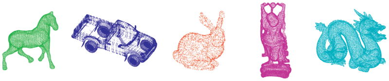
Different views of the 3D point sets used in this paper.
5.3.1 Quantitative Comparison: Motion Dynamics (Truck)
In this experiment, we demonstrate the importance of stochastic motion with our own implementation of a filtering scheme similar to that of [23]. Specifically, we employ deterministic annealing for our process and measurement noise. Moreover, we replace the ICP functional with our optimizer so as to mitigate any problem caused from the objective functional as well as to highlight the differences between each filtering setup. Last, we also compare the above algorithms to a multiple hypothesis-based testing technique (i.e., no dynamics in the current framework).
As described in Section 1, dynamics have a significant impact on the registration results. For example, in the case of 3D LADAR imagery [2], pose tracking algorithms involve segmentation of an object from a scene, which is then followed by point set registration. However, at a given instance of time, the object may be only partially seen and segmented. This results in the task of partial matching in the context of registration. More importantly, when facing occlusions or erratic behavior, the extracted point set can be inaccurately initialized.
To demonstrate this, we first extract a cloud of points from the front side of the truck, as seen in Fig. 8a, and center it with respect to the model. We then create 50 transformations. First, translations t⃗ = [tx, ty, tz] are generated from a normal distribution with each component having a standard deviation of half the range of the model. The rotation angle θ is then chosen randomly along the z rotation axis, but from a uniform distribution . In our comparison, we initialized the process and measurement noise as 0.7 * [max(model) − min(model)] and 0.3 * [max(data) − min(data)], respectively. The annealing rates were chosen to be 0.85 for the process noise and 0.7 for the measurement noise. Initial distributions were the same for each filtering setup.
Fig. 8.

The importance of stochastic motion. (a) Initialization. (c) Result with deterministic annealing model. (c) Result with no dynamical model. (d) Result with stochastic motion model.
For the case of a multiple hypothesis testing, the algorithm was able to register 13 scans. We ran our own implementation, similar to that of [23], multiple times (trials = 50) for the 50 transformations. Using 1,000 particles for the filter driven by process and measurement noise, we report a mean success rate of 25 and a standard deviation of 3.41 (over 10 trials). For the filtering method proposed in this work, which used only 100 particles, we report a mean success rate of 40.96 and a standard deviation of 1.91. The reasoning for such an improvement between the two particle filters can be explained by the fact that even with 1,000 particles, at times “good” particles were driven away from the global minima by the high noise. In the same respect, the deterministic noise also allowed for “bad” particles to diffuse to the correct global minima. Fig. 8 shows an example of when the proposed approach outperforms deterministic annealing and a multiple hypothesis testing.
5.3.2 Qualitative Results: Partial Nonoverlapping Data Sets (Bunny, Room)
An important task for many point set registration algorithms is the ability to properly register scans that exhibit only a partial overlap of the surface. In addition, depending on the acquisition of the point sets, the sampling of points may create inconsistencies in the correspondences across two sets of interest. In what follows, we use L = 7 with 100 particles.
We begin with the famed 3D models from Stanford Repository, which are composed of models whose scans are taken in succession. We have limited our registration experiment to those scans that exhibit a poor initialization or poor overlaps. In particular, Fig. 10 shows the successful registration of bun000 to bun045, bun000 to bun315, bud0 to bud336, and drag0 to drag96.
Fig. 10.

Partial scans of an apartment room. Note the severe initial alignments. Top Row: Initializations. Middle Row: Intermediate result of proposed approach. Bottom Row: Final result with proposed algorithm. (a) bun000 to bun315. (b) bun045 to bun315. (c) drag72 to drag120. (d) drag0 to drag96.
While Fig. 10 demonstrates the notion of a nonoverlapping surface, the scans are generally tested with “local” optimizers. Thus, we extend this experiment to scans of a room taken by a DeltaSphere-3000 laser scanner. In particular, the large rotational offset along with sampling density and partial structures creates difficult problems for point set registration. In Fig. 11, we show the successful registration of four scans of a room.
Fig. 11.

Partial scans of an apartment room. Note the severe initial alignments. Top Row: Initializations. Middle Row: Intermediate result of proposed approach. Bottom Row: Final result with proposed algorithm. (a) apt10 to apt3. (b) apt10 to apt4. (c) apt10 to apt9. (d) apt10 to apt7.
5.3.3 Quantitative Results: Performance Gain of Employing PF Algorithm (Horse)
In this example, we extensively test the algorithm’s performance in the case of large misalignment and large levels of noise. Moreover, we demonstrate the performance gain of employing our proposed particle filtering algorithm. First, we generate two series of 100 random transformations and apply them to a data set that is uniformly sampled from the model. The first series of transformations focuses on the case for which iterative techniques are commonly tested. In particular, we generate translations t⃗ = [tx, ty, tz] from a normal distribution with each component having a standard deviation of 30, i.e.,
(0, 30). This value is chosen according to the range of model points, ([−36, 33], [−67, 74], [−75, 82]). The rotation angle θ is then chosen randomly along the z rotation axis, but from a uniform distribution
. The second series of transformations is similar to the first set, except now the rotation angle is chosen from a uniform distribution
.
After a transformation is applied, the data set is sampled with replacement with Gaussian zero mean noise. The applied noise is
(0, 45), which is again chosen with respect to the dimensions of the horse. In this experiment, we generated noise levels of 5, 10, 25, and 35 percent substitution, and then we performed tests at each of the several varying noise levels. Further, the number of particles used is 100 with L = 7, and the initial distribution has the same spread for each random transformation.
Table 2 above presents the number of successful alignments of running just the optimizer presented in Section 2.1.2 as well as the particle filtering algorithm proposed in this work. Because of the random nature of particle filtering, the experiment was repeated over 50 trials with the same initializations. We report both the mean success rate, standard deviation, as well as the minimum and maximum successful alignments for each case. Interestingly enough, the particle filtering approach outperforms the iterative-based technique even in the case where the rotational angle is not extreme. One can then see the significant improvement in widening the narrow band of convergence for the particular case of large offsets and noise.
TABLE 2.
3D Performance Gain of Employing Proposed Particle Filtering Method in Conjunction with Proposed Local Optimizer under Varying Levels of Noise and Initialization
| Noise | Optimizer (θ< 60°) | P.F. (50 Trials). (θ< 60°) | Optimizer (θ< 120°) | P.F. (50 Trials) (θ< 120°) |
|---|---|---|---|---|
| 5 %. | 83 |
μ = 91.17 σ = 1.62 max = 94 min = 88 |
57 |
μ= 75.59 σ = 2.81 max = 83 min = 72 |
| 10 %. | 86 |
μ = 92.89 σ= 1.74 max = 97 min = 90 |
55 |
μ = 74.23 σ = 3.40 max = 80 min = 66 |
| 25 %. | 79 |
μ= 85.20 σ = 1.96 max = 88 min = 81 |
49 |
μ = 69.44 σ = 2.80 max = 73 min = 63 |
| 35 %. | 74 |
μ = 82.86 σ = 2.35 max = 86 min = 78 |
44 |
μ = 66.44 σ = 2.16 max = 71 min = 60 |
Number of “Successful” alignments is shown, where “Success” is denoted if ||t⃗||< 2 with a rotational offset θ⃗ < 2 degree is found for each scan pair.
5.4 Performance Analysis
The final experiment examines the time-performance analysis of our particle filtering approach. Specifically, we focus on the breakdown limit of the number of particles needed for accurate registration in the case of the experiment performed in Section 5.3.1. We ran this experiment with the same transformations, but with the additional particle sizes of 50 and 500. To ensure a notion of repeatability of success the number of trials was chosen to be 50. For the case of 500 particles, we report a mean success rate of 48, with a standard deviation of 1.15. Compared to 100 particles as previously tried, which we reported to have a mean success rate of 40.96 and standard deviation of 1.91, adding more particles increases the rate of success. In contrast, the “breakdown” limit was seen to be roughly 50 particles in which the algorithm’s efficiency decreases to a mean success rate of 30.16 with a standard deviation of 2.24. This can be seen for a challenging initialization in Fig. 9. In particular, a higher level of particles also enables the algorithm to converge at a slightly quicker rate.
Fig. 9.

Plot of the energy convergence of the proposed approach with respect to the iteration count for three different sample sizes.
Last, we report the execution time, iteration count, and other relevant information for each of the experiments performed in this paper in Table 3. It should be noted that our implementations of both the “local” optimizer and particle filtering algorithm were done in MATLAB v7.1 on an Intel Dual Core 2.66 GHz with 4 GB memory. Also, in relative terms, our implementation of the filtering algorithm using deterministic annealing averaged 1,228 sec over 50 iterations. This reduction in computational speed is due to nearest neighbor searches and unoptimized code. One final key note about the performance of our algorithm is its ability to reduce the sample size of particles. From this, both ICP and particle filtering can be currently parallelized onboard a tracking system in a much more efficient manner, where limitations occur in the need for resampling component of the particle filter.
TABLE 3.
3D Performance Gain of Employing Proposed Particle Filtering Method in Conjunction with Proposed Local Optimizer under Varying Levels of Noise and Initialization
| Experiment | Model Dimension | Number of Model Points | Number of Data Points | Avg. Number of Iterations | Time (in Sec) |
|---|---|---|---|---|---|
| P.F. Gain Performance (Horse) | ([−36,33],[−67,74],[−75,82]) | 1000 | 1000 | 15 | 18.3 |
| Motion Dynamics (Tacoma Truck) | ([−33.31,33.31],[−74.97,74.99],[−28.15,28.15]) | 1000 | 10000 | 36 | 64.60 |
| 2D Noise Comparison (Projected Bunny) | ≈([−14,13],[−12,17]) | 299 | 299 | 6 | 5.31 |
| 2D Partial Structures (Letter Search) | ([−16.2 20.8],[−24.32,15.68]) | 450 | 64 | 9 | 5.03 |
| 2D Geometric Assumptions (Cube) | ([58.04 30.98],[−56.29,−26.95]) | 383 | 50 | 7 | 3.17 |
| Partial Non-Overlap (bun045,bud96,..) | ≈([−23, 31],[12 70],(−16 35]) | 1000 | 1000 | 48 | 40.93 |
| Partial Non-Overlap (apt3,aptl0,..) | ≈([−222 141],[−97,135],[−65,41]) | 5000 | 5000 | 26 | 88.1 |
6 Conclusion and Future Work
In this paper, we cast the problem of pose estimation for point sets within a particle filtering framework that exploits the underlying variability in the registration process. This is done by estimating “motion” or uncertainty as local variations in pose parameters in the posterior. From this, a novel local optimizer based on the correlation measure is proposed and derived. The methodology was shown to be able to deal with partial structures, poor initialization, partial overlaps, and noise without making any geometric assumption on the point set density. Unlike [23], [24], [26], the method does not require an annealing schedule and drives the registration with information that is learned online through a stochastic diffusion model. As compared to the KC algorithm [32], our approach only considers a set of correspondences in a switching like fashion. This enables the algorithm to correctly align point sets when dealing with partial structures or with the matching of dense and sparse sets.
Some of our future work will focus on modifying the proposed approach to address nonrigid transformations. From a filtering and theoretical perceptive, this amounts to having an infinite dimensional state space. Given the generality of the above framework, one may adopt a nonrigid optimizer and invoke this in the measurement functional to estimate the deformation.
Acknowledgments
This work was supported in part by grants from the US National Science Foundation, US Air Force Office of Scientific Research, and US Army Research Office as well as by a grant fromthe US National Institutes of Health (NIH) (NAC P41 RR-13218) through Brigham and Women’s Hospital. This work is part of the National Alliance for Medical Image Computing (NAMIC), funded by the NIH through the NIH Roadmap for Medical Research, Grant U54 EB005149. Information on the National Centers for Biomedical Computing can be obtained from http://nihroadmap.nih.gov/bioinformatics.
Biographies

Romeil Sandhu received the bachelor’s and master of science degrees in electrical engineering from the Georgia Institute of Technology in 2006 and 2009, respectively. He is currently pursuing the PhD degree at the Georgia Institute of Technology under the supervision of Allen Tannenbaum. His current research interests include segmentation, pose estimation, and registration with applications to visual tracking. He is a student member of the IEEE.

Samuel Dambreville received the master of science degree in electrical engineering in 2003, the master’s degree in business administration in 2006, and the PhD degree in electrical engineering in 2008 from the Georgia Institute of Technology. His research interests include visual tracking and shape-driven techniques for segmentation. He was the recipient of the Hugo O. Schuck Best Paper Award at the 2007 American Control Conference. He is a member of the IEEE.

Allen Tannenbaum is a faculty member in the Schools of Electrical and Computer and Biomedical Engineering at the Georgia Institute of Technology. He is also a faculty member in the School of Electrical Engineering at the Technion-Israel Institute of Technology. His research interests include systems and control, computer vision, and image processing. He is a fellow of the IEEE.
Appendix. Minimization of the Proposed Optimizer
We first linearize both translation and rotation:
Then, reorganizing terms gives us:
where
Now, we can rewrite the above energy functional as
Taking the variation w.r.t. C yields
Footnotes
Unless explicitly stated, we consider an alignment successful, if the registration offset is <2 degree and the norm of translation offset is <2.
For information on obtaining reprints of this article, please send to: tpami@computer.org, and reference IEEECS Log Number TPAMI-2008-08-0548.
Contributor Information
Romeil Sandhu, Email: rsandhu@gatech.edu, School of Electrical and Computer Engineering, Georgia Institute of Technology, 313 Ferst Drive, Atlanta, GA 30318.
Samuel Dambreville, Email: samuel.dambreville@gatech.edu, School of Electrical and Computer Engineering, Georgia Institute of Technology, 313 Ferst Drive, Atlanta, GA 30318.
Allen Tannenbaum, Email: tannenba@ece.gatech.edu, School of Electrical and Computer Engineering and the School of Biomedical Engineering, Georgia Institute of Technology, 313 Ferst Drive, Atlanta, GA 30318, and the Department of Electrical Engineering, Technion, Israel Institute of Technology, Haifa, Israel.
References
- 1.Stanford Univ. Computer Graphics Laboratory. The Stanford 3D Scanning Repository. 1996. [Google Scholar]
- 2.Albota M, Aul B, Fouche D, Heinrichs R, Kocher D, Marino R, Mooney J, Newbury N, O’Brien M, Player B, Willard B, Zayhowski J. Three-Dimensional Imaging Laser Radars with Geiger-Mode Avalance Photodiode Arrays. Lincoln Laboratory J. 2002;13(2):351–370. [Google Scholar]
- 3.Besl PJ, McKay ND. A Method for Registration of 3-D Shapes. IEEE Trans Pattern Analysis and Machine Intelligence. 1992 Feb;14(2):239–256. [Google Scholar]
- 4.Chen Y, Medioni G. Object Modeling by Registration of Multiple Range Images. Image Vision and Computing. 1992;10(3):145–155. [Google Scholar]
- 5.Chui H, Rangarajan A. A New Algorithm for Non-Rigid Point Matching. Proc IEEE Conf Computer Vision and Pattern Recognition. 2000;2:44–51. [Google Scholar]
- 6.Chui H, Rangarajan A, Zhang J, Leonard CM. Unsupervised Learning of an Atlas from Unlabeled Point-Sets. IEEE Trans Pattern Analysis and Machine Intelligence. 2004 Feb;26(2):160–172. doi: 10.1109/TPAMI.2004.1262178. [DOI] [PubMed] [Google Scholar]
- 7.Dey T, Sun J. Normal and Feature Estimations from Noisy Point Clouds. Proc Foundations of Software Technology and Theoretical Computer Science. 2006;7:21–32. [Google Scholar]
- 8.Doucet A, de Freitas N, Gordon N. Sequential Monte Carlo Methods in Practice. Springer Verlag; 2001. [Google Scholar]
- 9.Eggert DW, Lorusso A, Fisher RB. Estimating 3-D Rigid Body Transformations: A Comparison of Four Major Algorithms. Machine Vision and Applications. 1997;9(5/6):272–290. [Google Scholar]
- 10.Fitzgibbon AW. Robust Registration of 2D and 3D Point Sets. Image Vision and Computing. 2003;21(13/14):1145–1153. [Google Scholar]
- 11.Gelfand N, Mitra NJ, Guibas LJ, Pottmann H. Robust Global Registration. Proc Symp Geometry Processing. 2005;255:197–207. [Google Scholar]
- 12.Goldberger J, Gordon S, Greenspan H. An Efficient Image Similarity Measure Based on Approximations of KL-Divergence between Two Gaussian Mixtures. Proc IEEE Int’l Conf Computer Vision. 2003:487–493. [Google Scholar]
- 13.Gordon N, Salmond D, Smith A. Novel Approach to Nonlinear/Nongaussian Bayesian State Estimation. IEE Proc Radar and Signal Processing. 1993;140(2):107–113. [Google Scholar]
- 14.Granger S, Pennec X. Multi-Scale EM ICP: A Fast and Robust Approach for Surface Registration. Proc European Conf Computer Vision. 2002;2353:418–432. [Google Scholar]
- 15.Horn B. Closed-form Solution of Absolute Orientation Using Unit Quaternions. J Optical Soc Am. 1987;4(1):629–634. [Google Scholar]
- 16.Huber DF, Hebert M. Fully Automatic Registration of Multiple 3D Data Sets. Image Vision and Computing. 2003;21(7):637–650. [Google Scholar]
- 17.Huber PJ. Robust Statistics. John Wiley & Sons; 1981. [Google Scholar]
- 18.Isard M, Blake A. Condensation—Conditional Density Propagation for Visual Tracking. Int’l J Computer Vision. 1998;29(1):5–28. [Google Scholar]
- 19.Jian B, Vemuri BC. A Robust Algorithm for Point Set Registration Using Mixture of Gaussians. Proc IEEE Int’l Conf Computer Vision. 2005;2:1246–1251. doi: 10.1109/ICCV.2005.17. [DOI] [PMC free article] [PubMed] [Google Scholar]
- 20.Johnson A, Herbert M. Using Spin Images for Efficient Object Recognition in Cluttered 3-D Scenes. IEEE Trans Pattern Analysis and Machine Intelligence. 1999 May;21(5):433–449. [Google Scholar]
- 21.Lakaemper R, Sobel M. Correspondences between Parts of Shapes with Particle Filters. Proc IEEE Conf Computer Vision and Pattern Recognition. 2008:1–8. [Google Scholar]
- 22.Li H, Hartley R. The 3D-3D Registration Problem Revisited. Proc IEEE Int’l Conf Computer Vision. 2007:1–8. [Google Scholar]
- 23.Ma B, Ellis RE. Surface-Based Registration with a Particle Filter. Proc Medical Image Computing and Computer-Assisted Intervention. 2004;3216:566–573. doi: 10.1007/11566465_10. [DOI] [PubMed] [Google Scholar]
- 24.Ma B, Ellis RE. Unified Point Selection and Surface-Based Registration Using a Particle Filter. Proc Medical Image Computing and Computer-Assisted Intervention. 2005;3749:75–82. doi: 10.1007/11566465_10. [DOI] [PubMed] [Google Scholar]
- 25.Makadia A, Patterson A, IV, Daniilidis K. Fully Automatic Registration of 3D Point Clouds. Proc IEEE Conf Computer Vision and Pattern Recognition. 2006;1:1297–1304. [Google Scholar]
- 26.Moghari M, Abolmaesumi M. Point-Based Rigid-Body Registration Using an Unscented Kalman Filter. IEEE Trans Medical Imaging. 2007 Dec;26(12):1708–1728. doi: 10.1109/tmi.2007.901984. [DOI] [PubMed] [Google Scholar]
- 27.Rathi Y, Vaswani N, Tannenbaum A, Yezzi A. Tracking Deforming Objects Using Particle Filtering for Geometric Active Contours. IEEE Trans Pattern Analysis and Machine Intelligence. 2007 Aug;29(8):1470–1475. doi: 10.1109/TPAMI.2007.1081. [DOI] [PMC free article] [PubMed] [Google Scholar]
- 28.Ristic B, Arulampalam S, Gordon N. Beyond the Kalman Filter: Particle Filters for Tracking Applications. Artech House; 2004. [Google Scholar]
- 29.Sandhu R, Dambreville S, Tannenbaum A. Particle Filtering for Registration of 2D and 3D Point Sets with Stochastic Dynamics. Proc IEEE Conf Computer Vision and Pattern Recognition. 2008:1–8. [Google Scholar]
- 30.Sofka M, Yang G, Stewart CV. Simultaneous Covariance Driven Correspondence (CDC) and Transformation Estimation in the Expectation Maximization Framework. Proc IEEE Conf Computer Vision and Pattern Recognition. 2007;14:1–8. [Google Scholar]
- 31.Stewart CV. Robust Parameter Estimation in Computer Vision. SIAM Rev. 1999;41(3):513–537. [Google Scholar]
- 32.Tsin Y, Kanade T. A Correlation-Based Approach to Robust Point Set Registration. Proc European Conf Computer Vision. 2004:558–569. [Google Scholar]