

Abstract
This paper presents a novel multiscale shape representation and segmentation algorithm based on the spherical wavelet transform. This work is motivated by the need to compactly and accurately encode variations at multiple scales in the shape representation in order to drive the segmentation and shape analysis of deep brain structures, such as the caudate nucleus or the hippocampus. Our proposed shape representation can be optimized to compactly encode shape variations in a population at the needed scale and spatial locations, enabling the construction of more descriptive, nonglobal, nonuniform shape probability priors to be included in the segmentation and shape analysis framework. In particular, this representation addresses the shortcomings of techniques that learn a global shape prior at a single scale of analysis and cannot represent fine, local variations in a population of shapes in the presence of a limited dataset.
Specifically, our technique defines a multiscale parametric model of surfaces belonging to the same population using a compact set of spherical wavelets targeted to that population. We further refine the shape representation by separating into groups wavelet coefficients that describe independent global and/or local biological variations in the population, using spectral graph partitioning. We then learn a prior probability distribution induced over each group to explicitly encode these variations at different scales and spatial locations. Based on this representation, we derive a parametric active surface evolution using the multiscale prior coefficients as parameters for our optimization procedure to naturally include the prior for segmentation. Additionally, the optimization method can be applied in a coarse-to-fine manner. We apply our algorithm to two different brain structures, the caudate nucleus and the hippocampus, of interest in the study of schizophrenia. We show: 1) a reconstruction task of a test set to validate the expressiveness of our multiscale prior and 2) a segmentation task. In the reconstruction task, our results show that for a given training set size, our algorithm significantly improves the approximation of shapes in a testing set over the Point Distribution Model, which tends to oversmooth data. In the segmentation task, our validation shows our algorithm is computationally efficient and outperforms the Active Shape Model algorithm, by capturing finer shape details.
Index Terms: Brain structures, schizophrenia, segmentation, shape representation, wavelets
I. Introduction
The characterization of local variations specific to a shape population is an important problem in medical imaging since a given disease often only affects a portion of the surface of an organ. In particular, one of the driving biological projects that motivates our work is the study of schizophrenia, a multifaceted illness affecting 1% of the U.S. population and consuming a significant portion of the health-care budget (estimates of yearly costs are 60 billion dollars) [1]. Yet the image-based clinical study of schizophrenia is only now beginning to take concrete form, primarily because neuroimaging techniques are finally providing a sufficiently detailed picture of the structure of the living brain and tracking the way the brain functions in controlled experimental settings. One important aspect of such an analysis of schizophrenia is the segmentation and shape analysis of selected brain structures, such as the hippocampus or the caudate nucleus, in order to find differences between groups of healthy and diseased patients.
Currently, such segmentations are typically carried out by hand. An automatic tool would be a great advance if it were to reliably and reproducibly segment cortical structures for multiple patients, across multiple time points. After the shapes are segmented the geometrical differences between brain structures of patients with schizophrenia and patients without can be studied. Many shape features have been proposed, some global, such as volume [2] or the shape index [3], some local such as point-to-point differences [4], and some at intermediate scales, such as the medial representation [5].
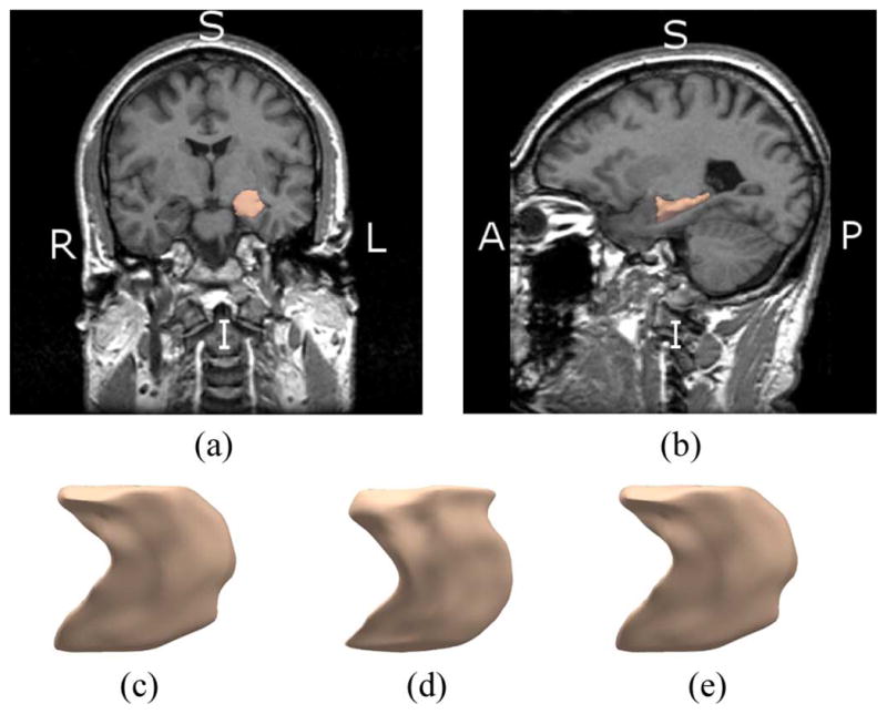
Fig. 1 shows a rendering of left caudate nucleus along with an MRI slice in the coronal and sagittal view, as well as three typical surfaces from our dataset. The caudate nucleus is located in the basil ganglia, a group of nuclei in the brain associated with motor and learning functions [6]. Fig. 2 shows the same information for the left hippocampus. The hippocampus is a part of the brain located inside the temporal lobe. It forms a part of the limbic system and plays a part in memory and navigation [7]. As can be seen in Figs. 1 and 2, those structures contain sharp features that could be important in shape analysis [8]. An automated segmentation of such structures must therefore be highly accurate and include relevant high frequency variations in the surface. Since shape representation is a key component of the segmentation, it must be descriptive enough to express shape variations at various frequency levels, from low harmonics to sharp edges. Additionally, a shape representation that encodes variations at multiple scales can be useful in itself as a rich feature set for shape analysis and classification.
Fig. 1.

(a), (b) Coronal and Sagittal view of left caudate nucleus. (c)–(e) Example of three shapes from left caudate nucleus dataset.
Fig. 2.
(a), (b) Coronal and Sagittal view of left hippocampus. (c)–(e) Example of three shapes from left hippocampus dataset.
As will be reviewed in Section II, medical object segmentation with deformable models and statistical shape modeling are often combined to obtain a more robust and accurate segmentation [9]–[13]. In that framework, a joint prior probability over shape parameters is learned using a training set in order to constrain the parameter values during the segmentation process. However, the degrees of freedom that can be expressed with the shape parameters and the number of training samples greatly influence how accurately the the prior probability can be estimated.
To address this issue, a decomposable shape representation targeted to the population seems natural, where the shape parameters are separated into groups that describe independent global and/or local biological variations in the population, and a prior induced over each group explicitly encodes these variations. Wavelet basis functions are useful for such a representation since they range from functions with global support to functions localized both in frequency and space, so that their coefficients can be used both as global and local shape descriptors, unlike Fourier basis functions or principal components over landmarks which are global shape descriptors. The use of spherical wavelet basis in medical imaging has been investigated for segmentation in 2-D imagery [14] but not yet for surfaces in 3-D imagery. This work addresses this gap and presents three novel contributions for shape representation, multiscale prior probability estimation, and segmentation. Finally, we should note that preliminary versions of the approach described in the present paper have appeared in the conference proceedings in [15] and [16].
The remaining sections of this paper may be summarized as follows. We first review related work in Section II. We then describe our shape representation based on the spherical wavelet transform in Section III. In Section IV, we detail the construction of a scale-space prior over the wavelet coefficients for a population of shapes and evaluate this prior in a reconstruction task. In Section V, we derive a parametric active contour segmentation flow based on the spherical wavelet representation and scale-space prior and evaluate this algorithm in a segmentation task. We conclude in Section VI with a discussion and future work.
II. Previous Work
A. Shape Representation
In this paper, we focus on 3-D brain structures that have boundaries that are simply connected surfaces (topological spheres). To conduct segmentation or shape analysis on such structures, it is useful to have a mathematical description of the boundary of the given structure. Two main approaches exist: to represent the boundary explicitly in a parametric form or implicitly as the level set of a scalar function. For the parametric form, the simplest representation is a set of N discrete 3-D points connected by a triangular mesh (piecewise linear surface). The full surface can be compactly encoded using 3N point coordinates and a connectivity list [17].
Other parametric representations use linear combinations of basis functions defined at the vertices of the mesh. In the work of Staib et al. [18], a Fourier parameterization decomposes the surface into a weighted sum of sinusoidal basis functions. One complexity of the technique is the choice of surface parameterization. More recent work has avoided the parameterization problem by first mapping the surface to the sphere and decomposing the shape signal using basis functions defined directly on the sphere. In the work of Brechbuhler et al. [19], a continuous, one-to-one mapping from the surface of an original object to the sphere is defined using an area-preserving mapping that minimizes distortions. The object surface can then be expanded into a complete set of spherical harmonics basis functions (SPHARM). Similar to the Fourier surface approach, the advantage of this representation is that the coefficients of the spherical harmonic functions of different degrees provide a measure of the spatial frequency constituents that comprise the structure. Partial sums of the series can be used to compactly represent selected frequencies of the object. As higher frequency components are included, more detailed features of the object appear. However, due to the global support of the spherical harmonic functions, the coefficients cannot be used to identify where on the surface the frequency content appears. Spherical wavelet functions address this shortcoming since they have local support at various scales. In [20] and [21], the authors showed that a spherical wavelet basis can capture shape changes with fewer coefficients than a spherical harmonic basis and can be used successfully for cortical surface shape analysis. In [22], spherical wavelets are used to analyze a manifold not topologically equivalent to a sphere by doing a nonbijective mapping between the manifold and the sphere via the normals. In [23], the authors also use a multiresolution approach to shape characterization but do not use spherical wavelets.
With the implicit representation, surfaces are the zero level set of a scalar function in ℝ3. The scalar function used is often a signed distance map. Implicit representations are less compact than the parametric representation but can represent any topology. This can be an advantage during the segmentation process since the implicit shape representation can naturally handle topological changes. However, in this paper we will be focusing on structures with the same topology and will therefore be using a parametric representation that is more compact and therefore more efficient during a surface evolution. We will discuss in Section VI the extension of our multiscale shape prior and segmentation algorithm to implicit shape representations.
B. Segmentation With Active Contours
By representing the shape of the segmented structure boundaries with a model and deforming the model to fit the data, deformable models offer robustness to both image noise and boundary gaps [9] and have been extensively studied and widely used in medical image segmentation, with good results. There are two types of deformable models, based on which representation is used for the model: parametric deformable models and geometric deformable models.
The classical parametric model is based on the snake formulation. See [9] and [24] for a detailed survey of snakes, their extensions, and their use in medical image analysis. Geometric deformable models [25]–[28] evolve a curve or surface using only geometric measures. Since the evolution is independent of the parameterization, the evolving curves and surfaces can be represented implicitly as a level set of a scalar function [29], [30]. As a result, topology changes can be handled automatically at the expense of a higher computational cost since the implicit shape representation is of higher dimension than the parametric representation. In this paper, since we will be segmenting brain structures of a fixed topology, our initial and final contour will remain of the same topology and we will therefore use the parametric model given its computational efficiency. One point of departure with the snakes model is that we will be deriving an evolution equation using the shape parameters directly as opposed to landmarks on the shape, in similar spirit to Tsai et al. [12].
Initial formulations of active contours, called “edge-based active contours,” combined smoothness constraints with image data forces sampled on the boundary of the model. One issue with edge-based active contours is that they are not robust to noise in the image and the gradient terms can stop the curve evolution at spurious edges. Recently, there has been a considerable amount of work on image segmentation using region-based curve evolution techniques. In those techniques, the force that influences the evolution of the curve depend on region statistics, inspired by the region competition work of Zhu and Yuille [31] and more recently the work of Chan and Vese [32] and Yezzi [33]. Our work uses the region-based active contour formulation in a parametric framework.
C. Shape Priors
Shape priors are commonly used to constrain shapes obtained during the segmentation and registration of biomedical images. Some of the first shape priors were based on local smoothness constraints [34] via elastic forces or combinations of global and local constraints [35] within the active contour framework. One limitation of these models is possible convergence to suboptimal shapes due to high flexibility in deformations. Statistical shape models were devised to overcome such drawbacks by learning a shape model from a training set.
In the Point Distribution Model (PDM) of Cootes and Taylor [17], a probability prior is learned from a training set of shapes by estimating a joint probability distribution over a set of landmarks on the shapes using principal component analysis (PCA). The joint probability distribution is assumed to be a multivariate Gaussian distribution. A covariance matrix is built from the data, and a diagonalization of the covariance matrix provides eigenvectors that are the principal axes of the distribution (also called principal modes) and the eigenvalues provide a bound on the subspace occupied by the shapes seen in the training set. This prior is then used in a parametric active contour segmentation algorithm called Active Shape Models (ASM) by projecting the evolving shape onto the space of eigenvectors and limiting the evolving shape to lie within a certain number of standard deviations of the eigenvalues seen in the training set. Shape priors in geometric active contours were introduced by Leventon et al. [11], where the landmarks are the pixels of the distance map implicitly representing the shape.
In ASM, the advantage of using the covariance matrix from landmarks in a training set is to restrict the segmentation task to a subspace of allowable shapes. However, it has two major limitations. First, it often restricts deformable shape too much, particularly if it has been trained on a relatively small number of samples since the number of principal components extracted from diagonalizing the covariance matrix is bound by the number of training shapes. Indeed, since the rank of the covariance matrix is at most K − 1, if there are K training shapes used to create the covariance matrix, then at most K − 1 eigenvectors (or principal modes) exist. Second, eigenvectors of the covariance matrix encode the most global modes of variation in the shapes, hence finer, more local variations of shapes are often not encoded given a limited training set.
To address this issue, the authors in Davatzikos et al. [14] have proposed a hierarchical active shape model framework for contours in 2-D medical imagery using standard 1-D wavelets, with convincing results. They use the wavelet transform [36] to produce a scale space decomposition of the signal. The authors apply a wavelet transform to the parametric functions (x, y, z) representing a deformable contour. The authors approximate the full covariance matrix of the wavelet coefficients as a a matrix that is block diagonal, when rearranging the coefficients in the right order. Coefficients that belong to the same band make up a diagonal block of the covariance matrix. Coefficients are grouped into bands using a logarithm tree to divide the space-frequency domain. This groups coefficients of the same scale and nearby spatial location in the same band, following the assumption that only coefficients close in space and scale are closely correlated. Each diagonal block can then be statistically modeled independently of the rest of the matrix and eigenvectors are extracted for each diagonal block, bringing the total number of eigenvectors to (approximately) B(K − 1) if there are B blocks and K training shapes. The eigenvectors corresponding to bands at coarse scales reflects global shape characteristics, whereas the eigenvectors corresponding to bands at finer scales reflect local shape characteristics at a particular segment of the curve. Using this technique, the authors show that a segmentation using the wavelet shape prior is more accurate than a segmentation with traditional active shape models.
D. Our Contributions
We propose to extend the framework by Davatzikos et al. to 3-D imagery in three novel ways. First, we describe a multiscale representation of surfaces in 3-D medical imagery using conformal mappings and a compact set of spherical wavelets targeted to the population we are analyzing. Second, we present a novel algorithm to discover optimal independent multiscale shape variations (bands) from the data by doing a spectral partitioning of coefficients based on correlation, instead of arbitrarily grouping coefficients close in space and scale together. Lastly, we derive an active contour segmentation algorithm in the space of the spherical wavelet basis functions in order to directly and naturally include the multiscale prior into the surface evolution framework.
In [15], we presented an application of spherical wavelets to the statistical analysis of a population of 3-D surfaces in medical imaging, by applying PCA analysis to a scale-space decomposition of the spherical wavelet coefficients representing the shapes. Our results showed that this type of multiscale prior outperformed PDM in a reconstruction task. In this paper, we present this technique and further compare it to another wavelet-based prior. We then present a novel segmentation framework using this 3-D wavelet representation and multiscale prior.
III. Shape Representation
A. Data Description
Throughout this work, we employ two key brain structures to illustrate our techniques and our results. We use a dataset of 29 left caudate nucleus structures and a dataset of 25 left hippocampus structures, from a 1.5 Tesla GE Echospeed MR system, coronal SPGR images, 124 slices of 1.5 mm thickness, voxel dimensions 0.9375 × 0.9375 × 1.5 mm. The MRI scans were hand-segmented by an expert neuroanatomist to provide ground truth segmentations for each structure. Each manual segmentation defined a 3D surface for each structure extracted by a standard isosurface algorithm.
B. Spherical Wavelets
A spherical wavelet basis is composed of functions defined on the sphere that are localized in space and characteristic scales and therefore match a wide range of signal characteristics, from high frequency edges to slowly varying harmonics [36]. The basis is constructed of scaling functions defined at the coarsest scale and wavelet functions defined at subsequent finer scales. A scaling function is a function on the standard unit sphere (
 ) denoted by ϕj,k :
→ ℝ where j is the scale of the function and k is a spatial index that indicates where on the surface the function is centered. A usual shape for the scaling function is a hat function defined to be one at its center and to decay linearly to zero. Fig. 3(d) shows a scaling function for scale j = 0. The color on the sphere indicates the value of the function ϕ0,k at every point on the sphere. As the scale j increases, the support of the scaling function decreases. A wavelet function is denoted by ψj,k :
→ ℝ. At a particular scale j, wavelet functions are combinations of scale j and (j + 1) scaling functions. Fig. 3(e)–(f) shows wavelet functions for different values of j and k. Note that the support of the functions becomes smaller as the scale increases. Together, the coarsest level scaling function and all wavelet scaling functions construct a basis for the function space L2
) denoted by ϕj,k :
→ ℝ where j is the scale of the function and k is a spatial index that indicates where on the surface the function is centered. A usual shape for the scaling function is a hat function defined to be one at its center and to decay linearly to zero. Fig. 3(d) shows a scaling function for scale j = 0. The color on the sphere indicates the value of the function ϕ0,k at every point on the sphere. As the scale j increases, the support of the scaling function decreases. A wavelet function is denoted by ψj,k :
→ ℝ. At a particular scale j, wavelet functions are combinations of scale j and (j + 1) scaling functions. Fig. 3(e)–(f) shows wavelet functions for different values of j and k. Note that the support of the functions becomes smaller as the scale increases. Together, the coarsest level scaling function and all wavelet scaling functions construct a basis for the function space L2
Fig. 3.

Visualization of recursive partitioning of icosahedron mesh and basis functions built on finest resolution mesh. (a) Initial icosahedron (scale 0). (b) Two recursive partitionings of icosahedron (scale 2). (c) Four recursive partitionings of icosahedron (scale 4). (d) Visualization of scaling function of scale level j = 0. (e) Visualization of wavelet basis function of scale level j = 0. (f) Visualization of wavelet function of scale level j = 2. For (d)–(f), color corresponds to value of function on the sphere.
| (1) |
A given function f :
→ ℝ can be expressed in the basis as a linear combination of basis functions and coefficients
| (2) |
Scaling coefficients λ0,k represent the low pass content of the signal f, localized where the associated scaling function has support; whereas, wavelet coefficients γj,m represent localized band pass content of the signal, where the band pass frequency depends on the scale of the associated wavelet function and the localization depends on the support of the function.
In this paper, we use the discrete biorthogonal spherical wavelets functions defined on a 3-D mesh proposed by Schröder and Sweldens [37], [38]. These are second-generation wavelets adapted to manifolds with nonregular grids. The main difference with the classical wavelet is that the filter coefficients of second generation wavelets are not the same throughout, but can change locally to reflect the changing (non translation invariant) nature of the surface and its measure. This means that wavelet functions defined on a mesh are not scaled and shifted versions of the function on a coarser grid, although they are similar in shape, in order to account for the varying shape of mesh triangles. The second-generation spherical wavelets that we use are defined on surfaces which are topologically equivalent to the unit sphere (
) and equipped with a multiresolution mesh. A multiresolution mesh is created by recursively subdividing an initial polyhedral mesh so that each triangle is split into four “child” triangles at each new subdivision (scale) level. This is done by adding a new midpoint at each edge and connecting midpoints together. This process is shown in Fig. 3(a)–(c). The starting shape is an icosahedron with 12 vertices and 20 faces, and at the fourth subdivision level, it contains 5120 faces and 2562 vertices. Any shape (not necessarily a sphere) that is equipped with such a multiresolution mesh can be used to create a spherical wavelet basis and perform the spherical transform of a signal defined on that mesh.
1) Discrete Spherical Wavelet Transform
The algorithm for the fast discrete spherical wavelet transform (FSWT) is given in [38]. Here, we sketch the transform algorithm in matrix form which gives a more compact and intuitive notation for the rest of this paper. In practice, we use the FSWT in our implementation.
If there exist N vertices on the mesh, a total of N basis functions are created, composed of N0 scaling functions (where N0 is the initial number of vertices before the base mesh is subdivided, with N0 = 12 for the icosahedron) and Nr wavelet functions for r = 1, … R where Nr is the number of new vertices added at subdivision r (N1 = 30, N2 = 120, N3 = 480, N4 = 1920 for the first four subdivisions of the icosahedron). In this paper, we will refer to all basis functions as wavelet basis functions as a shorthand.
In matrix form, the set of basis functions can be stacked as columns of a matrix Φ of size N × N where each column is a basis function evaluated at each of the N vertices. The basis function is evaluated at each of the N vertices. The basis functions are arranged by increasing scale (subscript j) and within each scale level by increasing spatial index (subscript k). Since the spherical wavelet functions are biorthogonal, ΦTΦ ≠ Id (the identity matrix), so the inverse basis Φ−1 is used for perfect reconstruction, since Φ−1Φ = Id.
Any finite energy scalar function evaluated at N vertices, denoted by the vector F of size N × 1, can be transformed into a vector of basis coefficients ΓF of size N × 1 using the Forward Wavelet Transform:
| (3) |
and recovered using the Inverse Wavelet Transform:
| (4) |
The vector of coefficient Γ is composed of coefficients associated with each basis function in Φ. It contains scaling coefficients as its first N0 entries, then wavelet coefficients associated with wavelet functions of scale zero for the next N1 entries, and so forth, all the way to wavelet coefficients of scale R − 1 for the last NR entries. Therefore, in total, the vector contains N entries. Next, we describe how to represent shapes using spherical wavelets.
C. Shape Representation With Spherical Wavelets
In this section, we explain how to equip a set of anatomical shapes with the correct multiresolution mesh structure in order to build wavelet functions directly on a mean shape that is representative of the population. We then explain how to encode a shape signal into wavelet coefficients.
1) Shape Remeshing and Registration
Before we can perform our wavelet analysis, we need to retriangulate and register all the surfaces in the dataset, so that they have the same mutiresolution mesh and mesh nodes at corresponding anatomical locations. Our approach to surface registration is based on the theory of conformal (angle-preserving) mappings [39], [40] of surfaces with spherical topology. Regardless of the degree of surface variation, such as variations in convexity to concavity, the method efficiently unfolds each surface, yielding an analytic one-to-one (conformal) mapping of each surface onto the sphere, and between each pair of surfaces by composition of mappings. Although we have had success with our conformal mapping approach, we note that the wavelet analysis presented here does not require this particular method of spherical mapping. Indeed, other techniques such as inflation [41], harmonic mapping with rectangular grids [19], circle packing [42], least squares mapping [43], and conformal mapping with parabolic equations [44] could also be used. The steps of our registration and remeshing technique ar as follows.
Step 1: Conformal Mapping
Let Σ be a surface of spherical topology we wish to register and remesh. As noted above, our registration method is based on complex variables and the conformal mapping of Riemann surfaces. The core of the algorithm requires the solution of a pair of sparse linear systems of equations and uses finite element techniques to solve an elliptic partial differential equation of the form
| (5) |
where Δ denotes the Laplace-Beltrami operator on Σ, p is an arbitrary point on Σ, f is the desired conformal mapping to the sphere
, δp is the Dirac delta function at p, and w denotes a complex conformal coordinate around p. See [39] for details. The resulting mapping f to the sphere can be made unique by specifying three points on Σ to be mapped respectively to the north pole, south pole, and an equatorial point on the sphere. In Appendix A, we describe our technique for automatically choosing these three points. Choosing these points consistently helps insure that corresponding surface locations are well registered within the caudate and hippocampus datasets. This is an approach that works well in practice with the caudate nucleus and the hippocampus. We hypothesize that this approach would work with other shapes that have a major axis, so other automatic point selection would have to be devised for more complex shapes.
This first step is illustrated in the first two columns of Fig. 4, where each row of the first column represents a different initial left hippocampus surface with Σ three automatically chosen control points. The color represents the z coordinate of Σ for reference. The second column shows the result of mapping each point on Σ to the sphere using the conformal mapping f. The sphere S then has the same triangulation as Σ. The color shown at the vertices of S is still the z coordinate of the corresponding vertex on Σ.
Fig. 4.

Illustration of remeshing step for two left hippocampus shapes. See Section III-C-1 for details.
Step 2: Area Correction
As pointed out in the early spherical mapping work of [19], conformal mappings may result in extreme distortion of area which needs to be corrected for certain applications. In particular, when remeshing a surface using a standard multiresolution mesh, large distortions in area can result in a nonuniform distribution of mesh nodes on the original surface and a loss of fine detail. To prevent this, we have implemented a simple method to adjust the conformal mapping to have better area-preservation properties. This technique ensures that the cumulative area of the vertices on the sphere between the south pole and any latitudes, normalized by the overall sphere surface area, is equal to the cumulative area of the same triangles on the shape, normalized by the overall shape surface area. This ensures that the triangle areas for the sphere and the shape are spread out proportionally from south to north pole. To achieve this, we translate the points on the sphere along their longitudes. The mathematical details of the technique are as follows. Let for n = 1, 2, …, N represent the mesh points on the sphere, indexed so that z1 = −1 ≤ z2 ≤ … zN = 1. Then, z1 is the south pole (0, 0, −1) and zN is the north pole (0, 0, 1). For each zn, the area of the region of the sphere south of the latitude through zn is given analytically by 2π(zn +1). This region corresponds to a region on the original surface Σ of area An, which can be calculated using the triangulation of Σ. In particular, A1 = 0 and AN = A, where A is the total area of Σ. If An/A = 2π(zn + 1)/4π for all n, then these areas on Σ and the sphere are spread out proportionally from south to north pole. This is unlikely to be the case in practice, so we adjust each point pn to get a new point p̃n by setting z̃n = (2An / A) − 1 and setting . This effectively spreads out the areas on the sphere in proportion to their original surface areas. The advantage of this approach is that the algorithm involved does not require iteration, as a functional minimization or flow technique would, and guarantees that the adjusted spherical mapping remains bijective. In the third column of Fig. 4, each row shows an adjusted spherical mapping. The color coding is again the z coordinate of the original surface shown in the first column. Comparison of the second and third columns to the first clearly shows that the third has a better distribution of area than the second. We note that although this method has produced satisfactory results for the surfaces we analyze here, more irregular surfaces may require additional area adjustments.
Step 3: Remeshing
We retriangulate
with the vertices of a subdivided icosahedron shown in Fig. 3(c). This yields a sphere with a new triangulation denoted by
 . If we apply the inverse mapping to the vertices of
, f−1(
) = ΣR, we then obtain a retriangulated version of the original surface Σ. After this transformation, the retriangulated shape ΣR has two nice properties: 1) it has the required mesh for spherical wavelet analysis and 2) it has a one-to-one mapping with a canonical spherical mesh, therefore providing one-to-one correspondence with other shapes that have this property. Note that this remeshing step maintains the initial correspondences. Before remeshing, all shapes have been mapped to the sphere and their spherical map is aligned on the sphere with the pole selection. The remeshing is done with the same mesh for all shapes, therefore the spherical map is still aligned after the remeshing step.
. If we apply the inverse mapping to the vertices of
, f−1(
) = ΣR, we then obtain a retriangulated version of the original surface Σ. After this transformation, the retriangulated shape ΣR has two nice properties: 1) it has the required mesh for spherical wavelet analysis and 2) it has a one-to-one mapping with a canonical spherical mesh, therefore providing one-to-one correspondence with other shapes that have this property. Note that this remeshing step maintains the initial correspondences. Before remeshing, all shapes have been mapped to the sphere and their spherical map is aligned on the sphere with the pole selection. The remeshing is done with the same mesh for all shapes, therefore the spherical map is still aligned after the remeshing step.
Step 4: Registration
After remeshing, all shapes have the same mesh with N vertices. A Procrustes transformation [45] can be applied to all shapes to register them in Euclidean space. This result of the Procrustes alignment is shown in Fig. 5(a)–(c) for the left hippocampus dataset and in Fig. 5(d)–(f) for the left caudate dataset. After Procrustes alignment, we denote shape i by a vector of size 3N × 1 (the first N entries are the x coordinates of the vertices, the next N entries are the y coordinates, and the last N entries are the z coordinates). After all K shapes are registered, the Mean shape is found with the following equation:
| (6) |
Fig. 5.

After remeshing, shapes are aligned with Procrustes alignment and mean shape is computed. (a) Left hippocampus surfaces before alignment. (b) Left hippocampus surfaces after alignment. (c) Left hippocampus mean shape computed from aligned shapes. (d) Left caudate surfaces before alignment (b) and left caudate surfaces after alignment (c). Left caudate mean shape computed from aligned shapes.
The mean shape for the left hippocampus dataset is shown in Fig. 5(c) and for the left caudate dataset in Fig. 5(f).
2) Spherical Wavelets on Mean Shape
After the spherical mapping and registration, all shapes in the population are equipped with the same multiresolution mesh, where each vertex of the mesh corresponds to the same anatomical location across shapes. Since the spherical wavelet functions used in this work can be defined on any surface of spherical topology with a multiresolution mesh, we can build the basis functions directly on the mesh of a mean shape for a population. This creates a set of basis functions adapted to the geometry of the mean shape, and therefore more specific to each shape in the population than if we had used bases functions built on a sphere. For each shape, we denote the matrix of basis functions built on the mean shape mesh as Φm. A scaling function for scale 0 and a wavelet function for scales 2 and 4 are shown in Fig. 6(a)–(c) on the mean shape of the left hippocampus population.
Fig. 6.

Visualization of basis functions constructed on mean shape at various levels. (a) Scaling function at scale 0. (b) Wavelet function at scale 0. (c) Wavelet function at scale 2. For all subfigures, the color corresponds to the value of the functions.
3) Encoding Shape Signal With Spherical Wavelets
We represent each shape in the population by encoding the deviation from the mean using the spherical wavelet transform. We first encode the variation from the mean for the ith shape with the signal vi of size 3N × 1
| (7) |
We then transform vi into a matrix of spherical wavelet basis coefficients Γvi with the forward spherical wavelet transform
| (8) |
where Φmis the wavelet basis functions evaluated on the mean shape for that population. Therefore, a shape is transformed into wavelet coefficients by taking the forward wavelet transform of the x, y, and z variation from the mean signal. The resulting vector of coefficients Γvi contains as the first N entries the wavelet encoding of the x coordinates of the shape, ranked from coarse scale to finer scales, and similarly for the next N entries that encode the y coordinates, and the last N entries that encode the z coordinate.
4) Filtering Shape Signal by Projection Onto a Reduced Set of Basis Functions
The representation presented so far allows us to represent the shape at various scale levels, by a filtering operation that projects the shape onto a limited set of basis functions. This can be done by creating a filter matrix P of size M × N, where M is the number of basis functions to keep. Each row of the matrix P keeps a particular basis function of index j by having entries of value zero, except for the jth entry that is set to one. The filtering (for all coefficients) is then performed with the following equation:
| (9) |
The resulting filtered coefficients
are of size 3M × 1. To display the filtered shape,
is first premultiplied by the transpose of
 to be of size 3N × 1 (the coefficients that correspond to the eliminated basis functions are zero), the inverse wavelet transform is applied and the mean shape is added
| (10) |
One example of this projection process is shown in Fig. 7(a)–(d) for the left caudate shape 1 and (e)–(h) for the left hippocampus shape 1. Fig. 7(a) shows the mean shape for the left caudate population. Fig. 7(b)–(d) shows the mean caudate shape plus filtered variations from the mean for shape 1. If only coarse scale basis functions are used Fig. 7(b), the resulting shape is coarse with low frequency variations from the mean shape. If basis functions of finer (higher) scale are added to the projection set, the resulting shape contains additional high frequency variations [Figs. 7(c), (d)]. The same information is shown for the hippocampus in Fig. 7(e)–(h). This type of filtering (or truncation) operation where a whole scale level is suppressed is commonly used with Fourier functions, such as spherical harmonics. However, one advantage of spherical wavelets is that due to the local support of its basis functions, a more granular truncation can be done, where only certain basis functions at a scale level are suppressed, instead of all the functions for that level. This allows for a more compact truncation, keeping only those functions that represent important information in the signal, at all scale levels. The next section explains how we do this in a principled way for a whole population of shapes.
Fig. 7.

Example of filtering operation for shape 1 of left caudate dataset and left hippocampus dataset. (a) Mean shape. (b), (e) Mean shape + low frequency variations (scales 0–2). (c), (f) Mean shape + low and medium frequencies variations (scales 0–3). (d), (h) Mean shape + all frequencies variations (scales 0–4).
IV. Multiscale Shape Prior
To build a prior that captures both global and local variations in the population, we first reduce the dimensionality of the Γi coefficients and keep only the coefficients that encode relevant variations in the training data. This process is described in Section IV-A. After truncation, we present a novel algorithm to learn the probability distribution of the nontruncated coefficients. This process is described in Section IV-B.
A. Coefficient Truncation via Power Analysis
Given the total power ||p||2 of the shape signal for a population, we would like to remove the basis functions that do not contribute significantly to that power. We define the population shape signal p (size N × 1) by
| (11) |
where selects the variation from the mean of vertex n of shape i along the x axis, and and along the y and z axis, respectively.
Since the wavelet basis functions are not orthonormal, we cannot directly apply Parseval’s theorem for spectrum analysis. Indeed
| (12) |
where are the coefficients of the spherical wavelet transform of p.
In order to still perform a power analysis, we wish to see the contribution of each wavelet basis function to the total power for the population ||p||2. We know that for a signal p sampled at N vertices of the mean shape
| (13) |
since . Then
| (14) |
The contribution of the kth wavelet basis function to the sum in (14) is therefore
| (15) |
where Φm(:, k) is the kth column of the basis matrix Φm and Γp(k) is the kth element of the coefficients vector Γp.
Since we wish to remove basis functions that have no effect on ||p||2, we remove those whose contribution c(k) is close to zero. Noting that c(k) can be both positive and negative, we rank the contribution of each basis by their absolute value from highest to lowest and truncate the lowest basis functions whose cumulative contribution is lower than 0.01% of the total power. Based on this analysis, we build a filter matrix
 that indicates which basis functions to keep to represent that population of shapes.
This truncation step leads to a nice compression property since the reduced set of basis functions match variations specific to a shape population, without introducing large error between the filtered shape and the nonfiltered shape. Table I shows the number of truncated basis functions and the average mean and maximum error between original shapes and their filtered version, using a filter matrix
specific to the shape population, for both the hippocampus and caudate dataset. The error is shown in millimeters. We show the amount of truncation and error for varying population size from 5 to 20. For the caudate dataset, between 958 and 1383 basis functions out of 2562 are truncated, depending on the number of shapes used to find
. This represents a compression level between 45% and 54%. With the truncation, the filtered shapes differ on average less than 0.2 mm from their unfiltered version. Fig. 8(a) shows the original caudate shape 1 and Fig. 8(b) shows the filtered shape (based on a 54% truncation level). The colormap shows the distance between the filtered and nonfiltered shapes. As can be seen in the figure, the truncation filtering does not seem to effect the shape significantly and all high scale variations are still present. For the hippocampus dataset, between 780 and 888 basis functions are truncated, representing a compression level between 30% and 35%. Again, filtered shapes differ less than 0.2 mm on average from their unfiltered version. Fig. 8(c) shows the original hippocampus shape 1 and Fig. 8(d) shows the filtered shape (based on a 35% truncation level). Again, the truncation filtering does not affect the shape significantly and all the finer scales variation are still present.
TABLE I.
| Dataset | \ Num Training | N=5 | N=10 | N=15 | N=20 |
|---|---|---|---|---|---|
| Caudate | |||||
| # initial fn. | 2562 | 2562 | 2562 | 2562 | |
| # truncated fn. (% truncation) | 1125 (44) | 958 (37) | 1050 (41) | 1383 (54) | |
| Avg. Max. Error (mm) | 0.83 | 0.77 | 0.67 | 0.60 | |
| Avg. Mean Error (mm) | 0.15 | 0.17 | 0.16 | 0.15 | |
| Hipp. | |||||
| # initial fn. | 2562 | 2562 | 2562 | 2562 | |
| # truncated fn. (% truncation) | 888 (35) | 820 (32) | 780 (30) | 888 (35) | |
| Avg. Max. Error (mm) | 0.73 | 0.71 | 0.77 | 0.75 | |
| Avg. Mean Error (mm) | 0.16 | 0.14 | 0.13 | 0.14 |
Fig. 8.

Result of filtering operation to create a reduced basis set. (a) Original caudate, shape 1. (b) Filtered caudate shape (54% truncation) with mean squared error from original shape as colormap. (c) Original hippocampus, shape 1. (d) Filtered hippocampus shape (35% truncation) with mean squared error from original shape as colormap.
Fig. 9 summarizes the steps from Sections III–IV-A to transform a shape into its reduced wavelet representation. Next, we detail the steps to learn the multivariate probability distribution of the reduced wavelet coefficients for a shape population.
Fig. 9.

Shape representation from Sections III–IV-B.
B. Multiscale Spherical Wavelet Prior
After finding a reduced set of basis functions for a population of shapes, we wish to estimate the multivariate probability distribution P(Γ*) of the wavelet coefficients for that population. Each shape of that population is then a random realization from P(Γ*).
1) Motivation
To model the variation in the data, we take advantage of the natural multiresolution decomposition of the wavelet transform and learn variations in the population at every scale level. This means that small scale variations in the data will not be overpowered by large scale variations, which would be the case if we were to apply PCA directly to all the vertices or to all the wavelet coefficients since PCA is a least squares fit that finds the first K −1 major (large scale) variations in a dataset of K shapes. By finding variations at separate scales, we find K −1 variations for each scale of analysis.
We computed the covariance matrix of wavelet basis coefficients for each scale and observed that the matrices were sparse. As a comparison, the covariance matrix of the coordinates of the vertices (used in PDM) is dense. For a given scale, we can refine our model by taking advantage of this decorrelation property and cluster correlated basis coefficients together, with the constraint that coefficients across clusters have minimum correlation. Coefficients in the same cluster then represent areas of the shape that have correlated variations in the population, for a given scale. Coefficients that do not belong to the same cluster do not tend to be correlated in the population. Since the wavelet coefficients across clusters are uncorrelated, they are also independent under the Gaussian assumption (inherent when we apply PCA analysis). Therefore, the overall joint probability function of the wavelet coefficients P(Γ*) can be modeled as the product of the joint probability functions of smaller uncorrelated clusters of coefficients. Practically, this means that we can apply PCA to each cluster of coefficients and we obtain modes of variations for each cluster at a given scale. This decomposition increases the number of variation modes (degrees of freedom) in the shape representation, but hopefully still captures existing correlation in the data by clustering together the coefficients that are correlated and learning their modes of variation.
We note that this hierarchical decomposition is inspired by the previous work of Davatzikos et al. [14] who used 1-D wavelet basis functions to analyze shape contours in 2-D imagery and performed a scale-space decomposition of the wavelet coefficients. However, their work assumes that coefficients associated with wavelet functions of the same scale that are also close in space are correlated to each other. In this paper, we relax the assumption that only spatial proximity would dictate correlation and find clusters directly based on the correlation that exists in the data.
In the next section, we show how to discover the clusters from the data. In Section IV-B-4, we show how to learn variations over every cluster and how to combine them into a multiscale prior.
2) Coefficient Clustering via Spectral Graph Partitioning
Fig. 10 shows a simple example used throughout this section to illustrate our clustering algorithm.
Fig. 10.

Illustration of band creation algorithm.
To cluster correlated wavelet coefficients, we use a spectral graph partitioning technique [46]. We use a fully connected undirected graph G = (Vj, E) where each node indexed by n ∈ Vj is a random variable that represents the coefficients associated with the nth wavelet basis function of scale j. Each wavelet basis function n has three associated coefficients per shape i that represent the x, y, and z variation, and those coefficicents are , and . For each shape i, we combine those three coefficient values associated with basis function n into one variable . Then, the random variable at node n is represented by its K realizations (K is the number of training shapes) Un = [u1(n), …, uK(n)].
The weight on the edge that connects node n and m is a function of similarity between those nodes and is denoted w(n, m). To define w(n, m), we first find the sample correlation and p-value between the random variables Un and Um
| (16) |
where is the sample mean of un, σUn the sample standard deviations of Un, and K is the total number of samples (number of shapes in the population).
With the correlation we compute an associated p-value that is the probability of getting a correlation as large as the observed value by random chance, when the true correlation is zero. If pn,m is small, then the correlation rn,m is significant. We pick a significance threshold of 0.05.
We then define the weight on the edge that connect nodes n and m to be
| (17) |
This similarity between the nodes can be represented as a matrix where each entry n, m is the value w(n, m). In Fig. 10, the similarity matrix for the hippocampus population for all nodes of scale 0 is shown at the top left. The lighter the entry (n, m), the more similarity between coefficients of basis n and m.
Using the normalized cuts technique [46], we find the optimal partitioning of the nodes of into two disjoint sets and such that nodes within a partition have the highest similarity and nodes across partitions have the lowest similarity. For example, in Fig. 10, nodes 2, 3, 5, 6, 7, 8, 9, 10, and 11 are put in the subgraph and nodes 1, 4, and 12 are put in the subgraph . We show the new similarity matrix where the node indices are reordered such that the first contiguous nodes belong to and the next contiguous nodes belong to . This effectively transforms the similarity matrix into a block diagonal matrix, where entries outside of the diagonal blocks have minimum correlation.
For each subgraph, we recursively iterate the normalized cuts until we reach a stopping criterion. The stopping criterion is based on the quality of the decomposition of each graph, validating whether the total correlation between the coefficients separated in two subgraphs A and B is less than a percentage p of the total correlation between coefficients in the combined set V. So, if V is partitioned into sets A and B, we ensure that
| (18) |
In practice, we use p ≤ 0.1. For example, in Fig. 10, subgraph is further subdivided into subgraphs and .
After the recursion, each subgraph represents a set of wavelet basis functions whose coefficients are correlated at that scale. We group these wavelet basis functions into a band, encoded by an index set Bj,b where j is the scale level of the band and b is the band index. For example in Fig. 10, a total of three bands were discovered for scale 0: Band B0,1 corresponding to the nodes in subgraph , Band B0,2 corresponding to the nodes in subgraph , and Band B0,3 corresponding to the nodes in subgraph .
3) Visualizing Clustering Results
The visualization of resulting bands on the mean shape can in itself be interesting for shape analysis by indicating which surface patches co-vary across the training set.
To visualize the band Bj,b, we visualize the cumulative support of all wavelet basis in band Bj,b on the surface of the mean shape. This can be done by using as a colormap the sum of the columns of Φm (the basis function matrix) indexed by Bj,b. The higher (lighter) values of the colormap then indicate where the wavelet basis functions in the band have support. This is shown in Fig. 10 at the bottom right for all three bands of scale 0. Band B0,1 indicates correlated variation at the anterior/lateral side of the hippocampus (the wider portion of the shape) for that population. Band B0,2 indicates correlated variation at the posterior/lateral side (the thinner portion) and Band B0,3 indicates variation on the medial side (the portion that appears at the bottom in the figure).
Fig. 11 shows the result of the recursive clustering for the first scale level for the left hippocampus data in the first two columns. We used 20 training shapes to create the graph. Each row corresponds to a scale level. The first column shows the initial similarity matrix for each level. The second column shows the resulting partitioned similarity matrix. As expected, the off-diagonal interband covariance is minimal. There are various band sizes, due to the fact that new bands are only recursively divided if condition (18) is met. The last three columns show the location of a selected band and the variation found within that band, as will be explained next.
Fig. 11.

Coefficient clustering and selected band variation visualization for hippocampus data.
4) Building Prior
The final step for building the prior consists of finding variations within each band of wavelet coefficients. We call this approach the wavelet distribution model (WDM).
Given a band index set Bj,b, we create a filter matrix Pj,b that selects the wavelet basis functions in the band Bj,b. We then select the wavelet coefficients corresponding to band Bj,b for shape using i the following:
| (19) |
The size of is 3|Bj,b| × 1, where |Bj,b| is the number of basis functions in Bj,b.
We learn the major modes of variations in a band just like in PDM, by calculating the mean
| (20) |
forming a shape matrix
| (21) |
and covariance matrix
| (22) |
and then diagonalizing the covariance matrix to find the eigenvectors (major modes of variation) Uj,b. Each column of Uj,b is an eigenvector of size 3| Bj,b | × 1 that represents an axis of variation for the coefficients Γ* j,b. In total for that band, we find 3|Bj,b | or K − 1 eigenvectors, whichever number is smaller.
To create the shape prior, we transform the eigenvectors back into the right dimensions
| (23) |
so that the only nonzero entries of U* j,b are at the indices corresponding to band Bj,b.
We can visualize the effect of the kth eigenvector for band b and scale j, U* j,b(k), by varying the shape wavelet coefficients along that eigenvector by an amount α* j,b(k)
| (24) |
and then recovering the shape with (10).
This process is shown for the hippocampus dataset in Fig. 11 for a selected band for four different scale levels. The eigenvectors of lower scale bands represent relatively global aspects of shape variability, whereas bands at finer (higher) scales represent higher frequency and more localized aspects of shape variability. Hence, our technique discovers shape variations at every scale, where the variations are all the eigenvectors of all the bands and does not favor the discovery of global variations over local variations. Additionally, our prior accurately encodes finer details even with small training sets, since if there are a total of B bands, there exist on the order of L = B(K − 1) eigenvectors, as opposed to just K − 1 eigenvectors when using PDM.
The full prior contains all the eigenvectors for all bands and all scales in a matrix U* of size 3M × L if there are L eigenvectors in total.
A shape i can then be represented with the full prior
| (25) |
where αvi (size L × 1) represents the coordinates of the wavelet coefficients of that shape in the eigenvector space.
To summarize, each shape ΣP is now represented with the following equation:
| (26) |
C. Evaluation of Multiscale Shape Prior
In this section, we evaluate the multiscale shape prior based on WDM and band decomposition for a shape reconstruction task. The basic idea is to learn a prior with a training set and to project shapes from a test set onto the prior to evaluate how close a projected test shape is to its ground truth.
We have three goals for the evaluation.
Compare the WDM prior using scale-band decomposition to WDM using only scale decomposition.
Compare both WDM priors to PDM.
Test the effect of noise on all priors.
We partition our data with N shapes randomly into T training samples and N−T testing samples, where T = []5, 10, 15, 20] and learn a shape prior from the training set. The prior for PDM consists of the mean shape and the eigenvectors of the landmarks on the shape. The prior for WDM using scale only consists of the mean shape, the mean wavelet coefficient vector, the eigenvectors for coefficients from each shape. The prior for WDM using scale and bands consists of the mean shape, the mean coefficient vector, the band indices, and the eigenvectors for coefficients from each band.
Once we learn the priors from a training set, we project each shape in the testing set onto the eigenvectors of the prior and translate the coordinates of the projected test shape to a point lying at a reasonable distance of the training data (±3 observed standard deviation). We then reconstruct the modified test shape. A mean squared error between the vertices of the ground truth and the reconstructed shape is calculated for all shapes in the testing set.
To test the robustness of each prior, we also test the reconstruction in the presence of noise. To add noise to the test shape, we displace each vertex according to a Gaussian distribution with mean zero and a standard deviation that is 5% of the bounding box of the object, as shown in Fig. 14 (columns 2 and 4), producing a shape with noise sn. Ideally, we would want the prior to not be affected by the noise and the reconstructed shape to be close to the ground truth (the shape without noise). To test this, we project the noisy shape onto the priors, and calculate the mean squared error between the reconstructed shape and the ground truth shape.
Fig. 14.

Reconstruction task for test shape using ten training shapes (first two columns) and a test shape using 20 training shapes (last two columns).
Figs. 12 and 13 show the maximum squared reconstruction error, averaged over all the shape in the testing set, for the various shape priors and various training set sizes of the hippocampus (Fig. 12) and caudate (Fig. 13) datasets. The left graph show the error using the ground truth as a projection onto the priors, the right graphs show the error using the noisy ground truth as a projection onto the priors (the error is then computed between the reconstructed shape and the original ground truth). As we can see in the graphs, the WDM prior with scale and band decomposition outperform the other techniques for all training set sizes. It is also interesting to see that all priors are minimally affected by Gaussian noise. Therefore, although the WDM prior with scale and band decomposition is more specific than PDM (meaning it represents a population more accurately), it is not more sensitive to noise.
Fig. 12.

Hippocampus dataset. (a) Max squared reconstruction error (averaged over testing shapes) for various training set sizes. (b) Max squared reconstruction error with noise projection for various training set sizes.
Fig. 13.

Caudate dataset. (a) Max squared reconstruction error (averaged over testing shapes) for various training set sizes. (b) Max squared reconstruction error with noise projection for various training set sizes.
As an example, Fig. 14 shows the Ground Truth shape, Noisy shape, and reconstruction with PDM and wavelet shape priors with ten and 20 training samples for the hippocampus dataset. The figures show the reconstruction when the Ground Truth shape is projected onto the prior (column 1 and 3) and when the Noisy shape is projected onto the prior (column 2 and 4). We see that details that appear in the WDM are lacking in the PDM reconstruction, especially on the posterior side (thinner part of the shape). When comparing WDM with scale only and WDM with scale and band decomposition, we see that the latter has a smaller error and contains finer details.
WDM outperforms PDM due to the fact that more degrees of freedom are better for the reconstruction task, asimple shape representation with as many degrees of freedom as the vertices would reconstruct any test shape perfectly (as long as there are enough vertices to represent the shape). The real test is during the segmentation task where too many degrees of freedom might yield incorrect segmentations in the presence of noise or corrupt image data, when an evolving shape leaks into areas of the MRI image that are not part of the shape. This justifies imposing a shape prior that limits the number of degrees of freedom, but can hopefully still capture the shape in the test data. We hypothesize that more degrees of freedom in the shape prior are better, as long as they still constrain the evolving shape to lie within a shape space targeted to the training set. Our approach attempts to discover more degrees of freedom, while keeping the shape prior faithful to the population under study by still captures existing correlation in the data at every scale.
Next, we explain how to use the WDM with band decomposition prior into an active surface segmentation framework.
V. Segmentation With Multiscale Prior
In order to exploit the multiscale prior, we derive a parametric surface evolution equation by evolving the PCA shape coefficients α directly. As the surface evolves to fit the image data, we constrain the weights α to remain within ±3 standard deviation of their values observed in the training set. The parameters of our model are the shape parameters α, as well as pose parameters that accommodate for shape variability due to a similarity transformation (rotation, scale, translation) which is not explicitly modeled with the shape parameters.
A. Pose Parameters
Given a surface mesh with N vertices Σ : [1, …, N] → ℝ4, expressed in homogeneous coordinates so that a mesh point is denoted by Σ(i) = xi = [xi, yi, zi, 1]T, a transformed surface Σ̃ is defined by
| (27) |
The transformation matrix T[p] is the product of a translation matrix with three parameters tx, ty, tz, a scaling matrix with one parameter s, and a rotation matrix with three parameters wx, wy, wz, using the exponential map formulation [47].
B. Shape Parameters
A surface point Σ(i) can be represented in the wavelet basis using the full formula (26)
| (28) |
where the function
 : [3N × 1] → [4 × N] rearranges a matrix to have the correct homogeneous coordinates and Φm(i, :) is a row vector of all the basis functions evaluated at point xi. The weight parameters α = [α1, …, αL] (where L is the total number of eigenvectors of the shape prior) are the shape parameters of our model.
By combining (27) and (28), the shape to be evolved is
| (29) |
where we use the tilde notation Σ̃ to indicate that Σ is evolving.
C. Segmentation Energy
The boundaries of the brain structures we are segmenting do not always exhibit a strong image intensity gradient. Therefore, using an edge-based force would not be sufficient to drive a correct segmentation. Region-based energies have been developed to adress this issue, where the force that influences the evolution of a contour depends on more global statistical information [12], [13]. We use a discrete version of the region-based force based on learned intensity statistics from the training set [13]
| (30) |
where R̃ is the region inside the evolving surface Σ̃ and the force is L(x̃) = − log(PI(I(x̃))/PO(I(x̃))) where I(x̃) is the image intensity at a point x̃ located inside the region R̃ of the evolving surface, PI(I(x̃)) is the probability that a point x̃ with intensity I(x̃) belongs to the interior of an object to be segmented in the image, and PO is the probability that the point belongs to the exterior of the object to be segmented. The segmentation energy is minimized when the surface evolves to include points that have maximum L (points that have a higher PI than PO). To estimate the probability density functions PI and PO from a training set, we collect sample voxel intensity values inside and outside the segmented shapes in a neighborhood of width ten pixels around the boundary and use Parzen windows [45].
The surface evolution is defined by a gradient flow of Σ that minimizes the energy in terms of the pose p and shape parameters α. We augment the parameters p and α with an artificial time parameter t and find gradient descent equations dp/dt and dα / dt by solving dE(p(t),α(t)) / dt = 0. We use the area formula [48] and then the divergence theorem to express the region integral in (30) as a surface integral and discretize the result to apply the result to a surface mesh (see Appendix B below for the full derivation). The gradient flow with respect to each pose parameter pk ∈ p is given by
| (31) |
with
Here,
 denotes the inward normal of surface point x̃i expressed in homogeneous coordinates and the image force L is evaluated at points on the surface boundary of Σ̃.
The gradient flow with respect to each shape parameters αk ∈ α is given by
| (32) |
where
Note that for a given αk, the evolution equation is projecting the image measure L onto the principal component U*(:, k) (or more precisely its backward wavelet transform into the space domain) corresponding to αk. See Appendix B for all of the details of the derivation.
D. Parameter Optimization via Multiresolution Gradient Descent
We can now use the gradient (31) and (32) to conduct a parameter optimization via gradient descent. Explicitly, the update equations are
| (33) |
| (34) |
where and are positive step size parameters, dp / dt is given in (31), and dα / dt is given in (32) and α(t+1), p(t+1) denote the values of the parameters α and p at the (t + 1)th iteration of the surface evolution.
We start with an initial shape and iterate between (33) and (34). We update the α parameters in a multiresolution fashion. Since each shape parameter αi corresponds to a band at a wavelet scale j, we first only update α coefficients corresponding to the coarsest level bands (j = 0). Once the coordinates of the evolving surface change less than a threshold value vα (in millimeters), we add the α parameters of the next scale level to the gradient and update (34). This results in a more stable segmentation since few global parameters are first updated when the shape is far from the solution and more localized parameters are added as the shape converges to the solution.
We start with (33) until (Σ̃t+1 − Σ̃t) < vp where Σ̃t is the evolving surface at time t and vp is a threshold value in millimeters. We then run (34) for one iteration and iterate the process. At each α iteration, we ensure that the value of the α parameters stays within ±3 standard deviation of the observed values in the training set. After each iteration, the updated shape and pose parameters are used to determine the updated surface.
E. Results of Segmentation
1) Experimental Setup
In this section, we test our segmentation algorithm that uses the region based force described in the previous section and evolves in the WDM shape prior space on the left caudate dataset and the left hippocampus dataset. We call this algorithm WDM/MSCALE. As a comparison, we also apply to the same dataset an active shape model (ASM) algorithm that uses the same region-based force but evolves in the PDM shape prior space (note that this is a modified version of the ASM algorithm published in [17] since we evolve the eigenvector weights directly instead of the mesh points). We call this algorithm PDM/ASM. We also test as a simple active contour algorithm that uses the same region-based force, but no shape prior, and call this algorithm NSP/AC (No shape Prior/Active Contour).
For both the WDM/MSCALE and PDM/ASM algorithms, we use the same training, testing shapes, and keep 100% of the eigenvectors for both the PDM and WDM representation. The landmarks for ASM are the vertices of the surface, after remeshing and alignment. These are the same vertices used to calculate the spherical wavelet coefficients used for the WDM shape representation. The shape parameters for ASM are the weights of the principal components that result from a PDM analysis.
Two main parameters of our technique are: 1) whether we truncate the coefficients, as described in Section II and 2) the number of training shapes. We vary both (1) and (2) for our experiments.
For the left caudate dataset and the left hippocampus, we learned a shape prior from varying sizes of training set shapes ([5, 10, 24] for the caudate dataset and [10, 15] for the left hippocampus), with and without truncation, and used the remaining shapes as a test set. We use spherical wavelet basis functions of scale up to j = 4. We learned the mean position pm of the caudate shapes in the MRI scans (in patient RAS coordinates, described in Appendix A). To initialize the segmentation, we use the mean caudate shape learned during the training phase and positioned it at position pm in the scan to be segmented.
For all three algorithms, the threshold parameters were chosen to be small enough to test for convergence. We pick vp = vα = 0.02 mm. The step size parameters also influence the convergence of the algorithm. Since we cannot directly interpret a change of α value in terms of euclidean distance, we ran an experiment with five test shapes and a binary image (where the voxels inside the test shape are set to 1 and outside are set to −1) and varied the parameter to look at its influence on the average mean error (in millimeters). The results are shown in Fig. 15 for the left caudate dataset, where the x axis shows the value . The figure shows that as increases ( decreases), the error gets smaller, until for both WDM/MSCALE and PDM/ASM. After that value, the error value stabilizes. A similar analysis made us choose parameters for translation and for scale and rotation.
Fig. 15.

Influence of step size on the mean error, using five test shapes for both PDM/ASM and WDM/MSCALE. x axis is value .
To measure the discrepancy between segmented shape (Σ) and ground truth (G) (obtained from the hand-segmented label-maps), we use the Hausdorff distance H(G, Σ) that measures the maximum error between the boundary of two shapes G and Σ, as well as the average surface error for the two shapes G and Σ. Both the Hausdorff distance and average surface errors are averaged over all shapes of a test set to obtain a global error measure for a training set size.
2) Results
To validate our algorithm, we first use the Ground Truth label-map as the image force in (31) and (32) by replacing L with a value of 1 inside the (known) object and −1 outside. The end goal is to validate whether the surface evolution converges to the right solution, given perfect image information. Since we are evolving in the space of the shape prior, the discrepancy between the PDM/ASM and WDM/Mscale algorithm is due to the expressiveness of the shape prior. Fig. 16 shows the result for the left caudate for a training set of 24 shapes. The final segmentation with the multiscale prior captures more of the shape and finer details than the ASM segmentation. Furthermore, we see that for as the scale level is increased for the α parameters, the Mscale segmentation is able to capture finer details. Fig. 17 shows the result for the left hippocampus for a training set of ten shapes. Again, the WDM/Mscale captures more details of the surface.
Fig. 16.

Left caudate dataset: surface evolution using ground truth label-map as image force for PDM/ASM (top rown) and WDM/Mscale (bottom row) algorithms, with 24 training shapes. Ground truth is shown in red (light-gray if seen in grayscale), evolving surface in blue (dark gray if seen in grayscale). (a) ASM, iter = 1. (b) ASM, iter =25. (c) ASM, iter = 122. (d) MSCALE, iter = 1. (e) MSCALE, iter = 96, levels 1–2 active. (f) MSCALE, iter = 122, levels 1–5 active.
Fig. 17.

Left hippocampus dataset: surface evolution using ground truth label-map as image force for PDM/ASM (top row) and WDM/Mscale (bottom row) algorithms, with ten training shapes. Ground truth is shown in red (light-gray if seen in grayscale), evolving surface in blue (dark gray if seen in grayscale). (a) ASM, iter = 1. (b) ASM, iter = 50. (c) ASM, iter = 102. (d) MSCALE, iter = 1. (e) MSCALE, iter = 50, levels 1–2 active. (f) MSCALE, iter = 94, levels 1–5 active.
To validate the full segmentation algorithm, we use the proposed image force in (30). The results of the validation for both algorithms are obtained by varying training set size and whether truncation is applied to the WDM shape prior or not. For a given training set size, the error is given as an average Hausdorff distance for all test cases in Fig. 20 for all algorithms and both structures. The error is also given as an average surface error for all test shapes in Fig. 21 for all algorithms and both structures.
Fig. 20.

Average Hausdorff error distance in millimeters, for all shapes of a test set, as a function of training set size for (a) left caudate and (b) left hippocampus dataset.
Fig. 21.

Average surface error distance in millimeters, for all shapes of a test set, as a function of training set size for (a) left caudate and (b) left hippocampus dataset.
We see that in all cases, the three algorithms with a shape prior outperform the active contour evolution without a prior. The results also show that both the WDM/MSCALE algorithms (with and without truncation) consistently outperform the ASM algorithm. Overall, the MSCALE algorithm without truncation outperforms the MSCALE algorithm with the hausdorff error, but not for the average surface error measure. This difference is more pronounced for the caudate dataset and small training set sizes. We hypothesize that the maximum error is most affected by the truncation since most of the truncated coefficients are at finer (higher) scales and high frequency differences are more visible with a maximum operator than an averaging operator. However, the effect of truncation needs to be further investigated in future experiments. The results also show that overall the PDM/ASM error is more affected by the training set size than the MSCALE error, as previously reported in [4].
Fig. 18 qualitatively compares the segmentation of the Left Caudate for a training set size of 24 shapes for both the PDM/ASM and WDM/MSCALE (with truncation) algorithms. The MSCALE algorithm is more accurate and captures finer details, especially at the tail of the caudate. Fig. 19 compares the segmentation of the Left Hippocampus for a training set size of ten shapes for both the PDM/ASM and WDM/MSCALE (with truncation) algorithms. We see that the MSCALE algorithm result is closer to the Ground Truth than the PDM/ASM result.
Fig. 18.

Left caudate dataset: surface evolution using density estimation as image force for ASM (top row) and Mscale (bottom row) algorithms, with 24 training shapes. Ground truth is shown in red (light-gray if seen in grayscale), evolving surface in blue (dark gray if seen in grayscale). (a) ASM, iter = 1. (b) ASM, iter = 32. (c) ASM, iter = 202. (d) MSCALE, iter = 1. (e) MSCALE, iter = 150, levels 1–2 active. (f) MSCALE, iter = 202, levels 1–5 active.
Fig. 19.

Left hippocampus dataset: surface evolution using density estimation as the image force for ASM (top row) and Mscale (bottom row) algorithms, with ten training shapes. Ground truth is shown in red (light-gray if seen in grayscale), evolving surface in blue (dark gray if seen in grayscale). (a) ASM, iter = 1. (b) ASM, iter = 134. (c) MSCALE, iter = 1. (d) MSCALE, iter = 102, levels 1–5 active.
The results show that the MSCALE representation with more degrees of freedom than ASM/PDM is able to better segment the test data (in terms of mean squared distance to the ground truth). However, the results also show that although the evolution without shape prior has more degrees of freedom, it has a higher mean and Haussdorff error when compared to our technique. These results suggest that more degrees of freedom are better, as long as they still constrain the evolving shape to lie within a shape space targeted to the training set. In this paper, we propose one type of scale-space decomposition based on correlation of spherical wavelet coecients at a given scale. It would be interesting to experiment with other types of decomposition, perhaps using other L2 basis functions or assuming more complex probability distributions for the shape features and using higher moments for decomposition.
We note that for both structures, the segmentation is not fully accurate due to nonperfect image statistics, meaning that that the statistics learned on the training set (the image term L based on PI, the probability of a voxel being inside the shape, and PO, the probability of a voxel being outside the shape) do not perfectly delineate the shape in the testing sets. Some voxels that belong to the Ground Truth test shape have a higher probability of being outside the shape than inside, and therefore the image force at that pixel is erroneous. Finding better image statistics as region-based forces is an active area of research, and other image terms could easily be substituted or added to L previously defined. The main focus of this paper, however, is to see whether the WDM prior can help drive a more accurate segmentation than a PDM prior, for a given image force. Both segmentation algorithms run on average 1 to 2 min (depending on the number of iterations needed for convergence) on a Pentium IV 2 GHz using nonoptimized MATLAB code and therefore have comparable running times. The prior computation time takes on average 1–2 min for PDM and 4–5 min for WDM for 20 shapes.
VI. Discussion
By using the spherical wavelet transform as shape representation, we have been able to take advantage of two types of decomposition: scale decomposition by using the transform structure and space decomposition by clustering coefficients based on correlation of the wavelet coefficients for the data we are analysizing. We have demonstrated that our spherical wavelet based technique WDM is a better shape prior when used in a segmentation task than ordinary PDM. We note that if the WDM technique is applied to other anatomical structures where the decorrelation property does not exist at particular scales, our technique will nicely default to including all coefficients from that scale into a single band.
Using this representation and prior, we presented a coarse-to-fine segmentation algorithm. Our results show that the proposed segmentation algorithm outperforms standard ASM. One advantage of the technique is the ability to evolve coarse scale parameters first, in order to quickly bring the evolving shape close to the solution and then evolving finer scale parameters to improve the fit. The technique is general and can be used with any kind of prior based on WDM, regardless of the decompositions used.
The general framework presented in this paper can be extended in several ways to benefit shape analysis and segmentation. So far, we have focused on a region-based energy in the formulation of the active contour given the lack of strong gradients around boundaries of subcortical structures, but it would be interesting to combine region-based forces with edge-based forces for other types of structures with stronger edge information. Another area of research would be to use other types of nonlinear prior estimation techniques over the wavelet coefficients, such as kernel PCA and generalized PCA. Additionally, our framework could be extended to implicit representations and a level set evolution by using standard 3-D wavelets directly on the grid. The scale-space decomposition algorithm to find the bands, as well as the segmentation algorithm, would translate nicely to this new representation. The wavelet transform could also provide a high compression for the implicit representation, given the redundancy present in a distance transform, typically used to implicitly represent curves and surfaces.
Our methodology finds independent shape variation processes at multiple scales and multiple locations by adaptively clustering correlated wavelet coefficients at each scale into bands. This shape representation itself and the band structures can be very interesting for shape analysis and classification. We can compare, for example, the band structures of a population with a neurological disease, versus a population without the disease. In our future work, we plan to investigate how the wavelet representation and the band structures can be used for classification. Our representation can also help physicians visualize variations specific to brain structures for a given population, at various scale levels.
Acknowledgments
The authors would like to thank M. Niethammer, E. Pichon, and the members of the MINERVA Biomedical Imaging Lab and the GVU Lab at Georgia Tech for their helpful suggestions and feedback throughout this work as well as the anonymous reviewers for their useful comment on drafts of this article. Information on the National Centers for Biomedical Computing can be obtained from http://www.nihroadmap.nih.gov/bioinfor-matics.
This work was supported in part by the National Alliance for Medical Image Computing (NAMIC), funded by the National Institutes of Health (NIH) through the NIH Roadmap for Medical Research under Grant U54 EB005149. The work of A. Tannenbaum and D. Nain was also supported by the NIH under Grant NAC P41 RR-13218 as well as a Marie Curie Grant from the EU through the Technion. The work of S. Haker was supported by the NIH under Grants R01CA109246, U41RR019703, P41RR013218, R01CA104976, R01CA111288, P01CA067165, and R01LM007861.
Appendix A
In this appendix, we show how to consistently pick three corresponding points (xN, xS, xE) on each shape of the hippocampus and caudate population in an automatic way. These three points will be used as boundary conditions of the conformal mapping so that xN is mapped to the north pole of the sphere, xS is mapped to the south pole, and xE to the point on the equator that intersects the Greenwich meridian. The steps are as follows.
Let Σ (ℝ → ℝ3) be a mesh in RAS patient coordinate space, with N points denoted x1 … xN. The RAS coordinate space signifies that the first axis is the patient’s left–right (LR) where left is negative and right is positive, the second axis is the patient’s posterior–anterior (PA), and the third axis is the patient’s inferior–superior (SI).
For each point xi on the mesh, let a(xi) be the sum of one-third of the triangles’ area that have xi at its vertex. Hence, a(xi) measures the portion of surface area attributed to vertex xi.
- Calculate the weighted mean of the surface
(35) - Center shape Σ around its mean
(36) - Extract the principal axes of the shape by finding the eigenvectors of the weighted moment tensor (xi (k) means we are taking the kth coordinate of xi)
(37) (38) (39) Reorder the eigenvectors to at most L → R, P → A, I → S. The axes are shown in Fig. 22 for three hippocampus and three caudate shapes. The magenta axis is LR, the blue axis is PA, and the green axis is IS.
Let xN be the farthest surface point from the center of the shape in the A direction of the PA axis (shown in blue in Fig. 22) and xS be the surface point in the P direction of the PA axis (shown in yellow in Fig. 22) and xE be the surface point in the L direction of the LR axis (shown in magenta in Fig. 22).
Since the xN and xS should be as far as possible, we change the xS location to be the farthest point (in geodesic distance) from xN. The distance is calculated on the mesh, using Dijkstra’s algorithm as an approximation of the geodesic distance. We show the result of this step on Fig. 23 for the same six shapes.
Fig. 22.

Example of principal axes and three points xN, xS, and xE found on three left hippocampus and left caudate shapes.
Fig. 23.

New point xS is found such that it is the farthest point on mesh from xN (in geodesic distance) for three left hippocampus and left caudate shapes shown in Fig. 22.
Appendix B
In this appendix, we give the main results of the volume-weighted gradient flow in [49] and [50]. Note that this derivation applies N to dimensions, but here we take the special case N = 3. Let R be an open connected bounded subset of ℝ3 (the region inside the surface) with smooth boundary Σ (the surface). Let φt be a family of embeddings, such that φ0 is the identity. Here, we consider the case where the given surfaces depend upon a parameter p that varies with time. Let L : ℝ3 → ℝ be a C1 function. Setting p0 for p(t)|t=0 and R(p(t)) := φt(R(p0)) and Σ(p(t)) := φt(R(p0)), we define the following family of L-weighted volumes:
| (40) |
| (41) |
where | J | is the determinant of the Jacobian resulting from the change of variables. Notice that the first integral depends on t, whereas the second integral does not depend on t via a change of variables [48].
Setting X(p0) = (dφt(x(p0))/dt)|t = 0
| (42) |
| (43) |
| (44) |
| (45) |
| (46) |
| (47) |
| (48) |
where we used a Taylor series expansion |Jφt(x)| = 1+ tdiv(X)+O(t2) so that (d|Jφt(x(p0))|/dt)|t=0 = div(X).
Then, using the divergence theorem
| (49) |
| (50) |
| (51) |
| (52) |
| (53) |
| (54) |
where
 is the inward normal to Σ.
To minimize E, and discretizing the result to deal with mesh surfaces, we obtain
| (55) |
Footnotes
Color versions of one or more of the figures in this paper are available online at http://ieeexplore.ieee.org.
Contributor Information
Delphine Nain, Email: delfin@alum.mit.edu, College of Computing, Georgia Institute of Technology, Atlanta, GA 30332 USA.
Steven Haker, Department of Radiology, Surgical Planning Laboratory, Brigham and Women’s Hospital, Boston, MA 02115 USA.
Aaron Bobick, College of Computing, Georgia Institute of Technology, Atlanta, GA 30332 USA.
Allen Tannenbaum, Email: tannenba@ece.gatech.edu, Electrical and Computer Engineering Department, Georgia Institute of Technology, Atlanta, GA 30332 USA and also with the Biomedical Engineering Department, Georgia Institute of Technology, Atlanta, GA 30332 USA.
References
- 1.NAMIC website. National Alliance for Medical Image Computing [Online] Available: http://www.na-mic.org.
- 2.Levitt JJ, McCarley RW, Dickey CC, Voglmaier MM, Niznikiewicz MA, Seidman LJ, Hirayasu Y, Ciszewski AA, Kikinis R, Jolesz FA, Shenton ME. MRI study of caudate nucleus volume and its cognitive correlates in neuroleptic-naive patients with schizotypal personality disorder. Amer J Psychiatry. 2002;159(7):1190–1197. doi: 10.1176/appi.ajp.159.7.1190. [DOI] [PMC free article] [PubMed] [Google Scholar]
- 3.Levitt JJ, Westin CF, Nestor PG, San-Jose R, Dickey CC, Voglmaier MM, Seidman LJ, Kikinis R, Jolesz FA, McCarley RW, Shenton ME. Shape of the caudate nucleus and its cognitive correlates in neuroleptic-naive schizotypal personality disorder. Biological Psychiatry. 2004;55:177–184. doi: 10.1016/j.biopsych.2003.08.005. [DOI] [PMC free article] [PubMed] [Google Scholar]
- 4.Xu S, Styner M, Davis B, Joshi S, Gerig G. Group mean differences of voxel and surface objects via nonlinear averaging. Proc IEEE Symp Biomedical Imaging. 2006:758–761. [Google Scholar]
- 5.Styner M, Lieberman JA, Pantazis D, Gerig G. Boundary and medial shape analysis of the hippocampus in schizophrenia. Med Image Anal. 2004;8(3):197–203. doi: 10.1016/j.media.2004.06.004. [DOI] [PubMed] [Google Scholar]
- 6.Wikipedia. [Last Accessed on, May 15, 2006];Caudate Nucleus [Online] Available: http://www.en.wikipedia.org/wiki/Caudate.
- 7.Hippocampus [Online] 2006 May 15; Available: http://www.en.wikipedia.org/wiki/Hippocampus.
- 8.Vetsa S, Styner M, Pizer S, Lieberman J, Gerig G. Caudate shape discrimination in schizophrenia using template-free non-parametric tests. Proc. 6th Int. Conf. Med. Image Computing Computer-Assisted Intervention (MIC-CAI); Montreal, QC, Canada. 2003. pp. 661–669. [Google Scholar]
- 9.Xu C, Pham DL, Prince JL. Handbook of Medical Imaging. Vol. 2. New York: SPIE Press; May, 2000. Medical image segmentation using deformable models; pp. 129–174. [Google Scholar]
- 10.Cootes TF, Taylor CJ. Combining point distribution models with shape models based on finite element analysis. Image Vis Comput. 1995;13(5):4039. [Google Scholar]
- 11.Leventon M, Grimson E, Faugeras O. Statistical shape influence in geodesic active contours. CVPR. 2000 Jun;2:1316–1325. [Google Scholar]
- 12.Tsai A, Yezzi AJ, Wells WM, III, Tempany C, Tucker D, Fan A, Crimson WEL, Willsky AS. A shape-based approach to the segmentation of medical imagery using level sets. IEEE Trans Med Imag. 2003 Feb;22(2):137–154. doi: 10.1109/TMI.2002.808355. [DOI] [PubMed] [Google Scholar]
- 13.Rousson M, Cremers D. Efficient kernel density estimation of shape and intensity priors for level set segmentation. Proc. 8th Int. Conf. Med. Image Comput. Computer-Assisted Intervention (MICCAI); 2005. pp. 757–764. [DOI] [PubMed] [Google Scholar]
- 14.Davatzikos C, Tao X, Shen D. Hierarchical active shape models, using the wavelet transform. IEEE Trans Med Imag. 2003 Mar;22(3):414–423. doi: 10.1109/TMI.2003.809688. [DOI] [PubMed] [Google Scholar]
- 15.Nain D, Haker S, Bobick A, Tannenbaum A. Multiscale 3D shape analysis using spherical wavelets. Proc. 8th Int. Conf. Medical Image Computing Computer-Assisted Intervention (MICCAI); LNCS. 2005. pp. 459–467. [DOI] [PMC free article] [PubMed] [Google Scholar]
- 16.Nain D. Shape-Driven Surface Segmentation Using Spherical Wavelets. 2006. pp. 66–74. [DOI] [PMC free article] [PubMed] [Google Scholar]
- 17.Cootes TF, Taylor CJ, Cooper DH, Graham J. Active shape models—Their training and application. Computer Vision and Image Understanding. 1995;61(1):38–59. [Google Scholar]
- 18.Staib LH, Duncan JS. Deformable fourier models for surface finding in 3D images. Proc 2nd Conf Vis Biomed Computing. 1992;1808:90–104. [Google Scholar]
- 19.Brechbühler C, Gerig G, Kübler O. Parametrization of closed surfaces for 3D shape description. CVIU. 1995 Mar;61(2):154–170. [Google Scholar]
- 20.Yu P, Segonne F, Han X, Fischl B. Shape analysis of neuroanatomical structures based on spherical wavelets. Human Brain Mapping (HBM) 2005;1:320–323. [Google Scholar]
- 21.Yu P, Han X, Segonne F, Buckner RL, Pienaar R, Golland P, Grant PE, Fischl B. Cortical surface shape analysis based on spherical wavelet transformation. Proc. IEEE Computer Soc. Workshop Math. Methods Biomed. Image Anal. (MMBIA); Jun. 2006; [DOI] [PMC free article] [PubMed] [Google Scholar]
- 22.Greenshields IR. 3D shape approximants via spherical wavelet decompositions. Proc. 14th Symp. Computer-Based Med. Syst; 2001. p. 31. [Google Scholar]
- 23.Jaume S, Ferrant M, Schreyer A, Hoyte L, Macq B, Fielding JR, Kikinis R, Warfield SK. Multiresolution signal processing on meshes for automatic pathological shape characterization. Proc. 4th Int. Conf. Med. Image Computing Computer-Assisted Intervention (MICCAI); LNCS. 2001. pp. 1398–1400. [Google Scholar]
- 24.McInerney T, Terzopoulos D. Deformable models in medical image analysis: A survey. Med Image Anal. 1996;1(2):91–108. doi: 10.1016/s1361-8415(96)80007-7. [DOI] [PubMed] [Google Scholar]
- 25.Whitaker RT. Volumetric deformable models: Active blobs. Visualization Biomed Comput. 1994:122–134. [Google Scholar]
- 26.Sethian J, Malladi R, Vemuri B. Shape modeling with front propagation: A level set approach. IEEE Trans Pattern Anal Mach Intell. 1995 Feb;17(2):158–175. [Google Scholar]
- 27.Caselles V, Kimmel R, Sapiro G. Geodesic active contours. Int J Computer Vision. 1997;22(11):61–79. [Google Scholar]
- 28.Kichenassamy S, Kumar A, Olver P, Tannenbaum A, Yezzi A. Conformal curvature flows: From phase transitions to active contours. Arch Rational Mechanics Anal. 1996;134:275–301. [Google Scholar]
- 29.Osher S, Fedkiw R. Level Set Methods and Dynamic Implicit Surfaces. New York: Springer Verlag; 2002. [Google Scholar]
- 30.Sethian JA. Level Set Methods and Fast Marching Methods. Cambridge, U.K: Cambridge Univ. Press; 1999. [Google Scholar]
- 31.Zhu SC, Yuille A. Region competition: Unifying snakes, region growing, and bayes/mdl for multiband image segmentation. IEEE Trans Pattern Anal Mach Intell. 1996 Sep;18(9):884–900. [Google Scholar]
- 32.Chan TF, Shen J, Vese L. Variational pde models in image processing. Notice AMS. 2003 Jan;50(1):14–26. [Google Scholar]
- 33.Yezzi A, Jr, Tsai A, Willsky A. A fully global approach to image segmentation via coupled curve evolution equations. J Vis Comm Im Rep. 2002;13:195–216. [Google Scholar]
- 34.Kass M, Witkin A, Terzopoulos D. Snakes: Active contour models. Int J Comput Vis. 1987;1(4):321–331. [Google Scholar]
- 35.Terzopoulos D, Metaxas D. Dynamic 3D models with local and global deformations: Deformable superquadrics. IEEE Trans Pat Anal Mach Intell. 1991 Jul;13(7):703–714. [Google Scholar]
- 36.Mallat S. Wavelet Tour of Signal Processing. New York: Academic; 1999. [Google Scholar]
- 37.Schröder P, Sweldens W. Spherical wavelets: Efficiently representing functions on the sphere. Proc Computer Graphics Proc (SIGGRAPH 95) 1995:161–172. [Google Scholar]
- 38.Schröder P, Sweldens W. Rendering Techniques ’95. New York: Springer Verlag; 1995. Spherical wavelets: Texture processing. [Google Scholar]
- 39.Angenent S, Haker S, Tannenbaum A, Kikinis R. Laplace-beltrami operator and brain surface flattening. IEEE Trans Medical Imag. 1999 Aug;18(8):700–711. doi: 10.1109/42.796283. [DOI] [PubMed] [Google Scholar]
- 40.Haker S, Warfield S, Tempany C. Lecture Notes in Computer Science. Vol. 3216. New York: Springer; 2004. Landmark-Guided Surface Matching and Volumetric Warping for Improved Prostate Biopsy Targeting and Guidance; pp. 853–861. [Google Scholar]
- 41.Fischl B, Sereno MI, Dale AM. Cortical surface-based analysis ii: Inflation, flattening, and a surface-based coordinate system. NeuroImage. 1999;9:195–207. doi: 10.1006/nimg.1998.0396. [DOI] [PubMed] [Google Scholar]
- 42.Hurdal MK, Stephenson K. Cortical cartography using the discrete conformal approach of circle packings. NeuroImage. 2004;23:119–128. doi: 10.1016/j.neuroimage.2004.07.018. [DOI] [PubMed] [Google Scholar]
- 43.Ju L, Stern J, Rehm K, Schaper K, Hurdal M, Rottenberg D. Cortical surface flattening using least square conformal mapping with minimal metric distortion. Proc 2nd IEEE Int Symp Biomed Imag. 2004:77–80. [Google Scholar]
- 44.Gu X, Wang Y, Chan TF, Thompson PM, Yau ST. Genus zero surface conformal mapping and its application to brain surface mapping. IEEE Trans Med Imag. 2004 Aug;23(8):949–958. doi: 10.1109/TMI.2004.831226. [DOI] [PubMed] [Google Scholar]
- 45.Duda R, Hart P, Stork D. Patten Classification. New York: Wiley-Interscience; 2001. [Google Scholar]
- 46.Shi J, Malik J. Normalized cuts and image segmentation. IEEE Trans Pattern Analysis Machine Intelligence. 2000 Aug;22(8):888–905. [Google Scholar]
- 47.Lepetit V, Fua P. Foundations and Trends in Computer Graphics and Vision. Vol. 1. Hanover, MA: Now; 2005. pp. 1–89. [Google Scholar]
- 48.Simon L. Proceeding of the Centre for Mathematical Analysis. Canberra: Australian National Univ; 1983. Lectures on geometric measure theory. [Google Scholar]
- 49.Pichon E, Tannenbaum A, Kikinis R. A statistically based flow for image segmentation. Med Image Anal. 2004 Sep;8(3):267–274. doi: 10.1016/j.media.2004.06.006. [DOI] [PMC free article] [PubMed] [Google Scholar]
- 50.Siddiqi K, Lauziere Y, Tannenbaum A, Zucker S. Area and length minimizing flows for shape segmentation. IEEE Trans Med Imaging. 1998 Apr;7(4):433–443. doi: 10.1109/83.661193. [DOI] [PubMed] [Google Scholar]