Bayesian hierarchical model of protein-binding microarray k-mer data reduces noise and identifies transcription factor subclasses and preferred k-mers

Abstract

Motivation: Sequence-specific transcription factors (TFs) regulate the expression of their target genes through interactions with specific DNA-binding sites in the genome. Data on TF-DNA binding specificities are essential for understanding how regulatory specificity is achieved.

Results: Numerous studies have used universal protein-binding microarray (PBM) technology to determine the in vitro binding specificities of hundreds of TFs for all possible 8 bp sequences (8mers). We have developed a Bayesian analysis of variance (ANOVA) model that decomposes these 8mer data into background noise, TF familywise effects and effects due to the particular TF. Adjusting for background noise improves PBM data quality and concordance with in vivo TF binding data. Moreover, our model provides simultaneous identification of TF subclasses and their shared sequence preferences, and also of 8mers bound preferentially by individual members of TF subclasses. Such results may aid in deciphering cis-regulatory codes and determinants of protein–DNA binding specificity.

Availability and implementation: Source code, compiled code and R and Python scripts are available from http://thebrain.bwh.harvard.edu/hierarchicalANOVA.

Contact: bojiang83@gmail.com or mlbulyk@receptor.med.harvard.edu

Supplementary information: Supplementary data are available at Bioinformatics online.

1 INTRODUCTION

Transcription factors (TFs) play a key role in the regulation of gene expression by activating or repressing transcription of their target genes. Regulatory specificity is achieved primarily by the recognition of specific DNA binding sites in the genome by sequence-specific TFs. Data on TF-DNA binding specificity are important for understanding how transcriptional regulation is encoded in cis-regulatory sequences in the genome.

TFs can be classified according to the structural class of their DNA-binding domains (Luscombe et al., 2000). TFs of the same structural class adopt the same fold in their DNA-binding domain and dock with their DNA binding sites in a similar manner. Because of these structural similarities, combined with sequence similarities because of the origin of TF families from ancient gene duplications and subsequent mutations, members of the same DBD class often, but not always, have similar DNA-binding sequence preferences (Badis et al., 2009). A DBD class can be further divided into subclasses, with more closely related proteins exhibiting more similar DNA-binding preferences. Understanding how highly similar members of a TF family attain both redundant and divergent regulatory functions remains a significant challenge (Grove et al., 2009).

Accurate and comprehensive data on DNA-binding sequence specificities are essential for investigations of regulatory targeting by TFs, including the identification of the molecular determinants of TF-DNA binding specificity. A variety of high-throughput technologies have been developed for determining TF-DNA binding specificity (reviewed in Bulyk and Walhout, 2012). Methods that provide data on in vivo TF occupancies in the genome, such as chromatin immunoprecipitation coupled with either DNA microarrays (ChIP-chip) or high-throughput sequencing (ChIP-Seq), provide data on both direct and indirect DNA binding by TFs (Gordân et al., 2009), which can vary across cellular or environmental conditions (Harbison et al., 2004). In contrast, approaches that determine DNA-binding specificities in vitro provide data on direct TF–DNA interactions, without the confounding effects of in vivo protein cofactors (Gordân et al., 2009).

Protein-binding microarray (PBM) technology is an in vitro approach for characterizing the DNA-binding specificities of proteins, by assaying the binding of a protein to a library of double-stranded DNA sequences immobilized on a DNA microarray (Bulyk et al., 2001). Universal PBMs contain synthetic DNA sequences designed to represent all possible k-mers, with commonly used array designs encompassing all possible 10 bp DNA sequences (k = 10) (Berger et al., 2006). Universal PBMs have been used in numerous recent studies to determine the DNA-binding specificities of hundreds of TFs from a wide range of organisms (Busser et al., 2012; Campbell et al., 2010; Grove et al., 2009), with major efforts on TFs encoded in the genomes of the yeast Saccharomyces cerevisiae (Badis et al., 2008; Gordân et al., 2011; Zhu et al., 2009) and mouse (Badis et al., 2009; Berger et al., 2008; Wei et al., 2010).

Universal PBMs contain 60 bp DNA probes, each of which contains multiple 10mers embedded within variable flanking sequence. For statistical robustness, binding preference scores are calculated for all 8mers, each of which is represented on at least 16 or 32 spots, for palindromic and non-palindromic 8mers, respectively, on the array. Analysis of universal PBM data using the Universal PBM Analysis Suite, including the Seed-and-Wobble algorithm (Berger and Bulyk, 2009; Berger et al., 2006), which was developed together with the universal PBM technology, involves background subtraction, various normalizations of the data and calculation of various binding scores for each 8mer, including the median fluorescence signal intensity over all probes that contain a particular 8mer and a rank-based PBM enrichment (E) score, ranging from −0.5 (worst) to +0.5 (best). The 8mer data can be used to derive a DNA-binding specificity motif, or position weight matrix (PWM) (Berger and Bulyk, 2009; Berger et al., 2006).

Analyses of large collections of universal PBM data have identified previously unknown diversity in the DNA-binding sequences recognized by TFs (Badis et al., 2009; Berger et al., 2008; Gordân et al., 2011). Hierarchical clustering of TFs according to their similarity in 8mer E-scores has permitted more precise identification of TF subclasses according to their DNA-binding specificities (Berger et al., 2008; Gordân et al., 2011; Wei et al., 2010). In addition, examination of k-mer-binding preferences within a TF family (here, defined as a group of closely related TFs belong to the same DBD structural class or the same subclass within a DBD class) has revealed sets of k-mers bound in common across the family (‘TF-common’ k-mers) and also sets of k-mers preferred by an individual member(s) of a TF family. To date, identification of such ‘TF-preferred’ k-mers has been performed in an ad hoc fashion, in manual investigations of individual sets of TFs that used various semi-arbitrary thresholds (Busser et al., 2012) combined with visual inspection (Berger et al., 2008; Gordân et al., 2011). Such TF-preferred k-mers may contribute to the distinct regulatory functions that distinguish members of a TF family.

Although hierarchical clustering has been used successfully for functional classification of gene expression profiling microarray experiments (Eisen et al., 1998) and for identification of TF subclasses based on PBM experiments (Berger et al., 2008; Gordân et al., 2011; Wei et al., 2010), the inclusion of unnecessary features that are irrelevant to cluster determination may degrade the results. This is especially the case for PBM experiments, where only a small fraction of k-mers measured by experiments are bound specifically by the profiled TF. Biclustering is a simultaneous similarity-based clustering approach that is able to detect subsets of features that exhibit consistent patterns over subsets of experiments (Cheng and Church, 2000; Gusenleitner et al., 2012); however, it does not directly provide a systematic classification of TF subclasses. Model-based methods for identifying and removing batch effects and other sources of variation have been developed for meta-analysis of high-throughput data, including microarray-based gene expression profiling experiments (Johnson et al., 2007; Leek and Storey, 2007, 2008; Leek et al., 2010, 2012). Direct application of such methods potentially could separate systematic background noise from identification of k-mers preferred by different TFs from PBM data.

Here, we present a Bayesian hierarchical analysis of variance (ANOVA) approach for modeling PBM k-mer data (here, 8mers). Our method identifies 8mers that score artifactually highly (‘sticky’ 8mers) for unknown reasons. Our approach for subsequently adjusting for these systematic biases improves overall PBM data quality and improves concordance with ChIP-chip data. Our modeling results in systematic identification of TF subclasses, simultaneously with their shared DNA-binding preferences, as well as the sequence preferences that distinguish them. Our TF subclassification results are consistent with classifications based on TF DBD sequence similarity. Our method also permits automated identification of TF-preferred k-mers within TF subclasses. Improved identification of TF-preferred k-mers will aid in studies of potential differences in the targeting of different genomic sites by paralogous TFs, and thus potentially how they may exert different regulatory functions. We anticipate that such modeling will aid in identification of genomic cis-regulatory codes (i.e. cis-regulatory sequence features that confer particular gene expression patterns) and will improve the quality of datasets for identification of the molecular determinants of TF–DNA sequence specificity.

2 METHODS

2.1 Datasets

2.1.1 PBM datasets

We downloaded universal PBM k-mer data and DBD structural class data from the UniPROBE database (Robasky and Bulyk, 2011), which hosts data generated by universal PBM technology on the in vitro DNA-binding specificities of proteins. The relative binding preference of a TF for each k-mer (here, k = 8) in universal PBMs is quantified by the PBM enrichment score (E-score), which is a modified form of the Wilcoxon–Mann–Whitney statistic (Berger et al., 2006). We refer to this as the observed E-score. We consider observed E-scores >0.35 as corresponding, in general, to sequence-specific DNA binding of the TF. In this study, we included 349 TFs from 19 DBD structural classes (e.g. homeodomain), with the criterion that there are at least three TFs per DBD class. Two of the downloaded PBM datasets are of particular interest in this study. One is a mouse TF dataset with 87 TFs from 12 DBD classes (filtered according to the above criterion from 104 TFs from 22 structural classes) previously described by Badis et al. (2009), in which PBM experiments were performed for each TF on two different versions of ‘all 10mer’ universal arrays, referred to as ‘version 1’ and ‘version 2’ [Agilent Technologies, Inc.; AMADID #015681 (Berger et al., 2008) and #016060 (Zhu et al., 2009), respectively], which were based on two different ‘all 10mer’ de Bruijn sequences. The other is a yeast TF dataset with 79 TFs from 10 DBD classes (filtered according to the aforementioned criterion from 89 TFs from 18 structural classes) in Zhu et al. (2009) for which ChIP-chip data (Section 2.1.2) are publicly available in Harbison et al. (2004) for 57 of these 79 TFs. We also included eight negative control experiments, corresponding to duplicate PBM experiments on each of array design versions 1 and 2, for glutathione S-transferase in binding buffer and, separately, for a mock in vitro transcription and translation reaction (Badis et al., 2009).

2.1.2 ChIP-chip datasets

We downloaded yeast ChIP-chip data from Harbison et al. (2004) for 352 ChIP-chip experiments for 207 TFs under various culture conditions (Harbison et al., 2004). We use the notation TF_cond to refer to the ChIP-chip experiment for transcription factor TF under environmental condition cond. For each ChIP-chip dataset, we defined the ‘bound’ intergenic regions to be those with ChIP-chip P < 0.001 and the ‘unbound’ intergenic regions to be those with ChIP-chip P > 0.5, as reported by Harbison et al. For 57 of these 207 TFs, PBM data are available in UniPROBE. We further restricted our analysis to ChIP experiments for which the ChIP ‘bound’ regions have been explained as being due to direct DNA binding by the profiled TF (Gordân et al., 2009); this requirement resulted in a final collection of 75 ChIP-chip datasets for 46 TFs.

2.2 Bayesian ANOVA decomposition of PBM k-mer data

2.2.1 Bayesian ANOVA model for identifying ‘TF-common’ and ‘TF-preferred’ k-mers

Given family membership (e.g. DBD structural class) of TFs, the DNA-binding specificity scores from PBM experiments can be decomposed into components attributable to at least three sources of variation: systematic biases across all PBM experiments, family-wise-binding preferences shared by members of the same TF family (i.e. ‘TF-common’ k-mers) (Berger et al., 2008; Busser et al., 2012) and k-mer-binding preferences specific to individual member(s) of a given TF family (i.e. ‘TF-preferred’ k-mers) (Berger et al., 2008; Busser et al., 2012). For PBM datasets from several diverse DBD classes, we used a Bayesian ANOVA model with hidden indicators to decompose PBM E-scores into different components and to infer the corresponding TF-common and TF-preferred k-mers systematically.

Specifically, for a TF family and a k-mer , we use () to indicate that the k-mer is preferred (disfavored) by members of that TF family, and if members of the family show no consistent preferred or disfavored binding for the k-mer. For a TF and a k-mer , we use () to indicate that the k-mer is preferred (disfavored) by the TF, and otherwise. Given family membership and the standardized E-score (standardized to have sample mean 0 and sample variance 1) of TF and k-mer , we assume the ANOVA decomposition:

(1)

where idiosyncratic noise 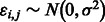, systematic background noise ,

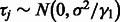We assign inverse χ² priors on , and , truncated normal priors on and and independent multinomial priors on indicators Ps and Qs (see Supplementary Fig. S2 for sensitivity analysis on the choices of priors). We used a Markov Chain Monte Carlo (MCMC) algorithm (Geman and Geman, 1984; Metropolis et al., 1953) to obtain posterior distribution of parameters and hidden indicators according to our ANOVA model [Equation (1)] (see Supplementary Methods for the MCMC algorithm and Supplementary Fig. S1 for diagnostics of its convergence). In the following study, we are especially interested in the posterior distribution of background noise , and indicators of family-wise and TF-specific effects.

2.2.2 Correcting k-mer data for systematic biases

Let be the posterior mean of calculated from Equation (1), and let be the standardized E-score of k-mer from a PBM experiment. To remove systematic biases, we subtract the posterior mean of the background noise from the corresponding standardized E-score, i.e. . Then, an E-score corrected for systematic biases can be obtained by transforming back to the original scale. We refer to this as the corrected E-score.

2.2.3 Evaluating the statistical significance of TF-preferred k-mers

For a pair of TFs and a given k-mer, we evaluate the statistical significance of its being TF-preferred by the intersection-union test (Berger and Hsu, 1996) with the null hypothesis that either none of the TFs exhibits preferred binding to the k-mer, or the pair have no difference in their binding preferences for the k-mer (see Supplementary Methods for details). We report all TF-preferred k-mers at an adjusted P < 0.05 by Benjamini–Hochberg correction (Benjamini and Hochberg, 1995) in an output text file and automatically create scatterplots showing the top n (user-specified setting) TF-preferred k-mers.

2.3 Bayesian partition model for identifying TF subclasses

2.3.1 Bayesian hierarchical partition model

The Bayesian ANOVA model introduced in the previous section assumes that TFs have been classified into families. In practice, DBD structural class can be used to define TF family memberships. However, members of the same DBD class do not always exhibit similar DNA-binding preferences. A collection of PBM datasets for TFs from the same DBD class provides a unique perspective to refine the classification of TFs into subclasses according to their DNA-binding sequence preferences. Here, we present a Bayesian model that simultaneously partitions TFs into subclasses that have similar DNA-binding profiles, and clusters k-mer DNA sequences into groups that are preferred by one or more TF subclasses.

Specifically, let be the standardized E-score of TF 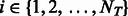and k-mer 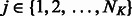, where is the number of PBM datasets for TFs from the same DBD class and is the total number of k-mers after collapsing forward and reverse complements ( 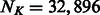for k = 8). Suppose is the unknown subclass of TF and is the unknown group membership of k-mer . For each group of the k-mers (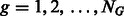), if the group is preferred by one or more TF subclasses and otherwise. Then, given and , we assume:

(2)

where follows if and if . We further assume that follows an inverse χ² prior with . As the total number of subclasses in a DBD class is unknown, we use a Dirichlet process prior on the subclass assignments . The prior probability of group assignment is given by , where . In this article, we show the results using and N_G = 100 (see Supplementary Fig. S3c for the sensitivity analysis on the choice of N_G and hyper-parameters , , and ).

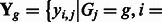
For each group of the k-mers, given , and hyper-parameters, we can integrate out (i.e. marginalize over) intermediate parameters in our hierarchical model [Equation (2)] to get an explicit expression of the probability , where is the collection of observed E-scores for k-mers in the group (Supplementary Methods). Combining with prior distributions of , and , we obtain the posterior distribution of , and given observed E-scores ,

(3)

We can draw from the posterior distribution [Equation (3)] iteratively using a collapsed Gibbs sampler (Liu, 1994) (see Supplementary Methods and Supplementary Fig. S3a and b for convergence diagnostics).

2.3.2 Motif model for aligning k-mer DNA sequences

We build a PWM to characterize the DNA-binding specificity of a group of k-mers (e.g. TF-common k-mers for a TF family). An element of PWM is defined as the probability of observing a nucleotide 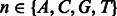at position 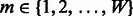, where is the pre-determined length of the PWM (here, for 8mer PBM data). Let 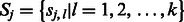be the DNA sequence of k-mer 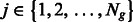in group , where is the number of k-mers in group , and is the alignment position of k-mer within the PWM, where . Here, we allow the k-mer sequence not to be fully ‘contained’ within a PWM but instead require that the alignments have an overlap of at least 4 nt. For example, means that the third position of k-mer is aligned with the start (i.e. 5′-end) of the PWM. The background probability of nucleotide , , is assumed to be 0.25. The probability of sequence being generated by the motif model is then given by:

(4)

where is an indicator function of event A. By assigning appropriate priors (Supplementary Methods), we can use a Gibbs sampling strategy (Geman and Geman, 1984; Lawrence et al., 1993; Liu, 2008; McCue et al., 2001) to iteratively update and based on the model shown in Equation (4). Finally, we construct a PWM based on the posterior modes of and generate a corresponding motif sequence logo (Schneider and Stephens, 1990).

3 RESULTS

We have developed a Bayesian ANOVA model to decompose 8mer PBM E-scores into background noise (i.e. artifactually high-scoring background k-mers), family-wise effects and experiment-specific effects, given a collection of PBM experiments and TF family classification based on DBD structural class. Below we start with the identification of artifactually high-scoring background k-mers, then describe the identification of TF subclasses based on the k-mer data and conclude with identification of experiment-specific effects in analyses aimed at improved identification of sets of k-mers bound preferentially by one TF as compared with a closely related TF (i.e. ‘TF-preferred’ k-mers).

3.1 Identification of artifactually high-scoring (‘sticky’) k-mers

From the ANOVA model [Equation (1)] described in Section 2.2.1, we can infer k-mer background noise based on their posterior means. Background noise constitutes a non-negligible component of E-scores with a standard deviation of 0.063, as compared with a standard deviation of 0.148 for E-scores (Fig. 1a). The posterior means of the variance and scale parameters , and are 0.647, 1.985 and 1.505, respectively. Examination of the sequences of the top 50 artifactually high-scoring k-mers, ranked according to their background noise and their E-scores across 357 experiments in our PBM datasets, indicates that AT-rich k-mers have artifactually high E-scores in nearly all PBM datasets for a diverse range of TF DBD classes (Fig. 1c); the most ‘sticky’ k-mer across a wide range of TF DBD classes is AAAAAAAA (Fig. 1b).

Fig. 1.

Artifactually high-scoring background k-mers. (a) Comparison of the distribution of k-mer background noise and the original (observed) E-scores. (b) Box plot of E-scores for the most ‘sticky’ k-mer (AAAAAAAA, collapsed with reverse complement TTTTTTTT) across all the available PBM datasets, including a set of negative control PBM experiments (Badis et al., 2009). (c) Sequence motif logo generated from the top 50 artifactually high-scoring k-mers and their E-scores across our PBM datasets. The multi-colored strip above the heatmap indicates each TF’s DBD class (from left to right): AP-2, AP2, ETS, Fork_head, GATA, HLH, HMG_box, HSF_DNA-bind, HTH, Homeodomain, IRF, MADS, Myb, RFX, SAND, ZnF_C4, bHLH, bZIP, Zf-C2H2 and negative control experiments. (d) (Top) Venn diagram comparing the number of ‘sticky’ k-mers with background noise larger than one standard deviation from two different ‘all 10mer’ de Bruijn sequence array designs; (Bottom) Venn diagram comparing ‘sticky’ k-mers identified from (Badis et al., 2009) and (Zhu et al., 2009), both of which used array design version 1

To compare the background noise of k-mers on different array designs, we calculated the k-mer background noise from the mouse TF PBM data from Badis et al. (2009), in which two different de Bruijn sequence array designs were used in PBM experiments for each TF; these are designated as array design versions 1 and 2 [AMADID #015681 (Berger et al., 2008) and #016060 (Zhu et al., 2009), respectively]. Comparison of the ‘sticky’ k-mers (i.e. those with background noise larger than one standard deviation of the original E-scores, which is 0.148 for version 1 and 0.153 for version 2) from this dataset indicates that (Fig. 1d) the two different array versions exhibit different numbers of ‘sticky’ k-mers, and that array design version 2 is noisier (i.e. has a larger number of ‘sticky’ k-mers) than version 1 (see Supplementary Figs S4 and S5 for additional comparisons of these two array versions). The two different array designs exhibited some differences in k-mer background noise (Pearson correlation coefficient r = 0.65; Supplementary Fig. S5a) as compared with independent experiments using the same array design (Pearson correlation coefficient r = 0.88; Supplementary Fig. S5b), for example, although AAAAAAAA is artifactually high scoring in both version 1 and version 2 datasets, CCCCGCCC is found to be ‘sticky’ only in version 1 datasets (Supplementary Fig. S4a). The top 20 artifactually highest scoring k-mers, together with their noise levels, from each of these two array versions are listed in Supplementary Figure S4c. To further investigate this effect, we compared the results from the Badis et al. mouse TF PBM data with the set of ‘sticky’ k-mers that we identified in analysis of a separate, yeast TF PBM dataset (Zhu et al., 2009), both of which used version 1 arrays. We observed significant overlap in the ‘sticky’ k-mers identified in these different datasets (Fig. 1d); differences in these sets of ‘sticky’ k-mers could be due to differences in protein sample preparation, experimental variation and differences in the representation of different DBD classes among the TFs that were tested in PBMs in the Badis et al. (2009) versus Zhu et al. (2009) studies.

3.2 Correction for artifactually high-scoring background for ‘sticky’ k-mers

As described in Section 2.2.2, we correct the E-score of each k-mer by subtracting its background noise from the original (observed) E-score. For example, for PBM data for the yeast TF Rpn4 published in Zhu et al. (2009), the observed E-scores and their corresponding background noise are highly correlated (Pearson correlation coefficient r = 0.71; Fig. 2a); subtracting the background noise from the E-scores reduced this correlation to 0.26. Comparison of the motif logo generated from the 68 k-mers with observed E-scores >0.35 with the logo generated from the same number of top scoring k-mers after correction for background noise shows that the quality of the motif greatly improves by correcting the E-scores for systematic biases (Fig. 2b).

Fig. 2.

Correction for artifactually high-scoring background k-mers. (a) Scatterplot of k-mer observed E-scores and background noise for yeast TF Rpn4. The blue dotted line indicates the original threshold of E ≥ 0.35. Red points indicate specifically bound 8mers after background correction. The correlation between E-scores and background noise diminishes from 0.71 to 0.26 after correction. (b) Improvement in motif quality for Rpn4 after correction for k-mer background noise

3.3 Evaluation of corrected k-mer E-scores as compared with ChIP-chip data

We used in vivo ChIP-chip–binding data to further evaluate the effect of background noise correction of PBM E-scores. Specifically, we first applied background noise correction to the yeast PBM data from Zhu et al. (2009), and then assessed whether this resulted in an improvement in scoring of regions called as ‘bound’ in the Harbison et al. (2004) ChIP-chip data for the same TF. Briefly, for a given TF and a given intergenic sequence, we first calculated an occupancy score by summing PBM median signal intensities for each k-mer with an observed E-score >0.35 (Zhu et al., 2009). We used these PBM-based occupancy scores to rank the intergenic sequences within the ChIP-chip ‘bound’ and ‘unbound’ regions for each ChIP-chip dataset, and then calculated the corresponding area under the receiver operating characteristic curve (AUC statistic). We repeated this same AUC calculation using the corrected E-scores. For comparison, we rank k-mers by their corrected E-scores and score the intergenic sequences using the same number of top-ranked k-mers as in the calculation with the original (observed) E-scores. In practice, the background correction of a new PBM experiment is based on the estimation from previous experiments; to accurately evaluate this process, we used an independent mouse TF PBM dataset (with the same array design) from Badis et al. (2009) to calculate k-mer background noise.

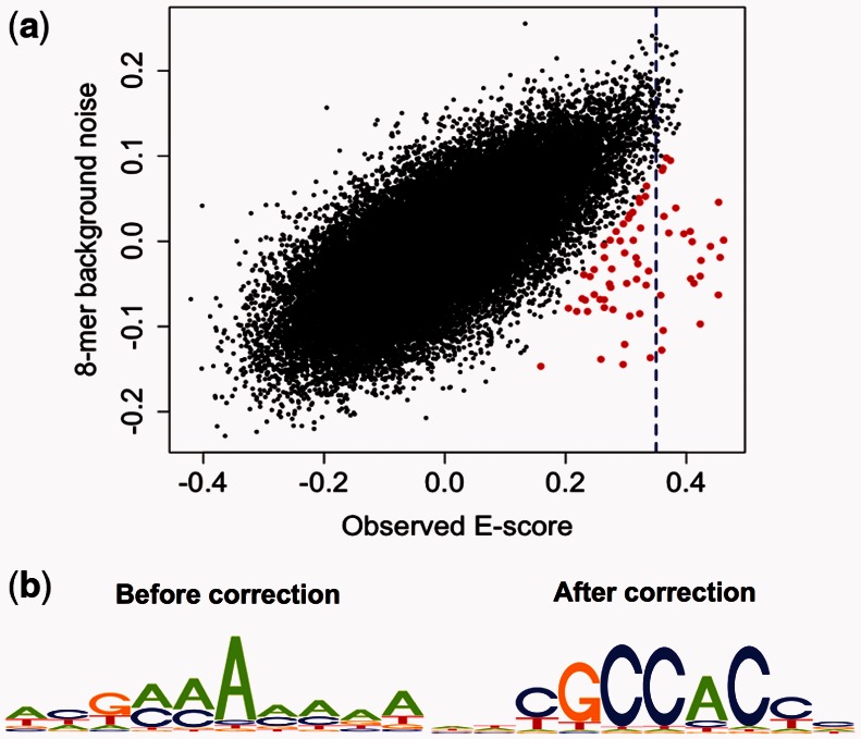
Overall, use of the corrected E-scores resulted in a statistically significant increase (P = 2.8 × 10⁻⁴ by Student’s t-test) in AUC statistics (Fig. 3). Some ChIP-chip datasets exhibited a sharp increase in AUC by using the corrected E-scores, for example, the AUC for Rpn4 increased from 0.573 to 0.749 for ChIP-chip data for a highly hyperoxic condition (RPN4_H2O2Hi) and from 0.680 to 0.910 for ChIP-chip data for a mildly hyperoxic condition (RPN4_H2O2Lo). Moreover, PBM datasets with relatively few high-scoring k-mers and low AUC values in such ChIP-chip analysis showed a uniform increase in AUC with the use of corrected E-scores; this observation is consistent with the hypothesis that the effect of k-mer background noise is more prominent in PBM datasets for TFs with relatively weaker binding signal. Any decreases in AUC value from using corrected E-scores were minor (<6%), and in one extreme case—Yap6, for which use of corrected E-scores resulted in a decrease of 6.0% from the original AUC value—the difference seems to be because of AT-rich ‘sticky’ k-mers that are bound sequence specifically by certain TFs, such as Sum1, which seems to provide for indirect binding of the ChIP-profiled TF (i.e. Yap6) to DNA (Gordân et al., 2009).

Fig. 3.

Comparison of corrected PBM k-mer data with ChIP-chip experiments. The relative change in AUC values by using corrected E-scores is plotted against the original AUC values before background noise correction. ChIP-chip datasets for which the use of corrected E-scores resulted in at least 10% change in AUC value are indicated with TF_condition names

3.4 Identification of ‘TF-common’ k-mers

By using the ANOVA decomposition model, we are able to identify groups of k-mers bound in common across the family (‘TF-common’ k-mers). For example, k-mers with high posterior probabilities for being TF-common have uniformly high E-scores for TFs in the ETS DBD class and relatively low E-scores for TFs in all the other DBD classes (Fig. 4a). The PWM constructed from these k-mers indicates a shared binding specificity for the ETS DBD class (Fig. 4a, top). Characterization of TF-common k-mers for other DBD classes (GATA, HLH, HMG-box and homeodomains) are given in Supplementary Figures S7–S10. Posterior distribution of family-wise effects and numbers of TF-common k-mers for all the DBD classes are given in Supplementary Figure S6.

Fig. 4.

Categorization of TF subclasses for the ETS DBD class. (a) TF-common k-mers for the ETS DBD class and their corresponding E-scores across our PBM datasets. The multi-colored strip above the heatmap is as in Figure 1c. (b) Pairwise posterior probabilities for clustering 22 mouse ETS factors based on the partition model described in Section 2.3.1. (c) Hierarchical clustering of 22 mouse ETS factors based on two groups of 8mers identified as subclass-preferred. (d) Classification of members of the ETS DBD class by aligning ETS-domain peptide sequences using the ClustalW algorithm. TFs marked with red boxes in (b), (c) and (d) show a strong preference for the core sequence GGAT relative to other members of the ETS DBD class

3.5 Identification of TF subclasses based on similarity of PBM k-mer data

Our Bayesian hierarchical partition model allows for categorization of TF subclasses based on DNA-binding preferences, which can simultaneously determine common binding sequences for each subclass. Previously, Berger et al. discovered separate DNA-binding specificity subgroups by considering the overlap among top 100 highest-affinity 8mers for homeodomains (Berger et al., 2008). Distinct binding patterns were also identified by manually examining 8mers with E-scores greater than a threshold score of 0.45. Our model-based analysis of homeodomains not only shows subclassification that is consistent with the results of Berger et al. (2008) but also systematically characterizes the common binding sequences for different subclasses of homeodomains (Supplementary Fig. S11).

We further applied our model to determine subclasses and their DNA-binding specificities in the ETS DBD class. Classification of 22 mouse ETS factors by hierarchical clustering (Fig. 4c) over two groups of 8mers identified in our analysis as being preferred by ETS subclasses is in general consistent with the classification obtained by aligning ETS-domain peptide sequences using the ClustalW algorithm (Fig. 4d), and it is broadly similar to the results obtained in Wei et al. (2010), in which the similarity between DNA-binding specificity motifs was obtained using the minimum Kullback-Leibler divergence between the multinomial distributions defined by the motifs. Notably, motifs generated according to subclass-preferred 8mers (Fig. 4c) are different from the motif generated from the TF-common k-mers (Fig. 4a). A subclass of the ETS factors with similar ETS-domain peptide sequences according to ClustalW shows a specific binding preference to a consensus sequence ACCGGAT (marked by a red box in Fig. 4c). Interestingly, members of this subclass can be distinguished further according to their binding preferences for the consensus sequence CCGGT. Differential binding preference by ETS factors for the core sequence GGAT has been observed previously (Wei et al., 2010), where its molecular basis was explored. By automatically identifying 8mers that have the most distinct binding patterns, our model is able to characterize the binding specificities among members of the ETS DBD class in more detail.

3.6 Identification of ‘TF-preferred’ k-mers

Highly similar members of a TF family can show different DNA binding sequence preferences. For example, the homeodomains Lhx4 and Lhx2 both bind most preferentially to the canonical sequence TAATTA, but they differ in their preferences for other k-mers (Berger et al., 2008). In Figure 5a, we show the DNA-binding specificity motifs for 8mers that are identified as TF-preferred by Lhx2 but not Lhx4, and for those identified as TF-preferred by Lhx4 but not Lhx2, according to our ANOVA model described in Section 2.2.1. At the same time, we also applied the procedure described in Section 2.2.3 to search for TF-preferred k-mers based on their statistical significance calculated by an intersection-union test. To have a sufficiently large sample size, we focused on TF-preferred 6mers in this study, and our tests are based on observed E-scores of 8mers containing a given 6mer. Analyses based on observed E-scores yielded nearly identical results as those based on corrected E-scores, as the differences between E-scores for a pair of TFs for the same k-mer are invariant to correction. The top three TF-preferred 6mers (each at P < 1.0 × 10⁻⁷) found by this analysis in a pairwise comparison of Lhx2 and Lhx4 are apparent as off-diagonal points in a scatterplot of 8mer E-scores (Fig. 5b). Of note, the TF-preferred 6mers identified by our model-based approach are consistent with TF-preferred 6mers identified by the intersection-union test. All four 6mers (TAATGA and TAACGA for Lhx2 and TAATCA and TAATCT for Lhx4) identified in (Berger et al., 2008) by a primarily manual approach are also significant in our new, automated analysis (Supplementary Fig. S12). In addition, our automated analysis finds additional TF-preferred k-mers, for example, it finds TAATGG as a statistically significant TF-preferred 6mer (P = 6.9 × 10⁻¹⁷) for Lhx2 and CAATCA as a statistically significant 6mer (P = 1.2 × 10⁻²³) for Lhx4, in a pairwise comparison of those two TFs. Note that our analysis identifies CAATCA as preferred by Lhx4 in comparison with both Lhx2 and also with Lhx3 (Supplementary Fig. S13).

Fig. 5.

Model-based identification of TF-preferred k-mers. (a) Scatterplot of 8mer E-scores comparing Lhx2 and Lhx4. The 8mers containing each of the top three most significantly TF-preferred 6mers from a direct comparison of Lhx2 and Lhx4 are highlighted in colors, revealing clear systematic differences in the binding by Lhx2 or Lhx4 to these sequences. (b) Sequence motif logos of TF-preferred 8mers for Lhx2 (left) and Lhx4 (right). Sequence motifs were generated as described in Section 2.3.2 using 8mers (with equal weights) that are identified by our ANOVA model as TF-preferred by one TF but not the other

4 DISCUSSION

Accurate high-resolution datasets on the binding preferences of TFs for comprehensive collections of DNA sequences are essential for understanding the nature of protein–DNA binding specificity and how those specificities are used in transcriptional regulatory codes encoded in genomes. In this study, we developed a Bayesian model-based approach for analyzing k-mer TF-DNA binding specificity data obtained from universal PBM experiments (Berger et al., 2006). Our model decomposes k-mer data (here, 8mers) into artifactually high-scoring 8mers, 8mers bound in common by a TF family and those bound preferentially by a particular member(s) of a TF family (TF-preferred k-mers). Adjusting PBM 8mer E-scores for the identified systematic biases improved overall PBM data quality and correlations with in vivo TF binding data obtained by ChIP-chip (Harbison et al., 2004). The TF subclasses identified by our modeling approach are consistent with TF subclasses based on TF DBD protein sequence similarity. TF-preferred k-mers are identified in an automated and systematic fashion by our model, without relying on visual inspection, manual curation or arbitrary thresholds; our model captures TF-preferred k-mers previously identified through a combination of such other methods (Berger et al., 2008; Busser et al., 2012), while being more comprehensive in identifying statistically significantly TF-preferred k-mers. Systematic identification of TF-preferred k-mers should help to reduce investigator bias in searching for TF-preferred k-mers and should aid in studies aimed at investigating the potential regulatory significance of TF-preferred versus TF-common k-mers (Busser et al., 2012; Gordân et al., 2011).

Although our analysis identified 8mers that tend to score artifactually highly in the universal PBM datasets that we examined, on its own, it does not provide an explanation for these observations. We investigated the various data normalizations that are performed on the universal PBM data, but we did not find any of them to contribute to artifactually high scores for these 8mers. We cannot exclude the possibility that these ‘sticky’ 8mers constitute a distinct set of non-specific sequences that are bound by numerous TFs more preferentially than truly nonspecific or even disfavored sequences. Determining the underlying cause of these ‘sticky’ 8mers will require additional experimental studies in the future.

To distinguish family-wise-binding effects from systematic biases, our ANOVA model [Equation (1)] requires a collection of TFs from diverse DBD classes and a sufficient number of TFs from each DBD class (at least three in this study). Estimation of k-mer background noise given a limited number of experiments (e.g. when adopting a new array design or platform) can be challenging. In this study, we focused our analysis on the observed E-scores because of the robustness of the E-score to experimental variation (Berger et al., 2006). Future development of non–rank-based approaches might allow for improved classification of TFs and k-mers.

In this study, we analyzed data from two specific universal array designs, synthesized based on two different de Bruijn sequences, each of which covers all 10mers. Our model could be applied to k-mer data generated using other universal array designs, including those based on higher-order de Bruijn sequences that comprehensively cover longer k-mers (Philippakis et al., 2008). Moreover, our approach is not limited to array designs based on de Bruijn sequences, but rather it can be applied to any datasets using PBMs or other assays for which binding scores for k-mers are generated.

Numerous studies have focused on different TF structural classes, with the goal of identifying recognition rules underlying protein–DNA binding specificity (Benos et al., 2002; De Masi et al., 2011; Noyes et al., 2008; Suzuki and Yagi, 1994). Precise classification of TFs according to their DNA-binding sequence preferences together with identification of those sets of preferred sequences, as provided by our modeling approach, will permit more detailed studies of the molecular determinants of TF-DNA binding specificity. Improved identification of k-mers bound preferentially by different TF family members will aid in investigations of what amino acid residues in the proteins correlate with differences in preferences for binding different k-mers.

Many studies of DNA regulatory elements have searched for combinations of motifs enriched within known or putative cis-regulatory elements (Warner et al., 2008), including investigations of whether there are preferential spacings or orientations of how the TF binding sites are arranged within promoters (Beer and Tavazoie, 2004; Senger et al., 2004) or transcriptional enhancers (Arnosti and Kulkarni, 2005). Moreover, how different TF family members achieve their distinct regulatory effects is still not well understood; TF-preferred k-mers constitute one mechanism by which paralogous TFs can attain distinct regulatory roles (Busser et al., 2012; Fong et al., 2012; Hollenhorst et al., 2009). More accurate, precise data on the DNA-binding sequence preferences of different TFs, in particular paralogous TFs, will be important for more detailed investigations of cis-regulatory codes.

The Bayesian hierarchical ANOVA modeling approach we present in this study is general and could be applied to other data types, beyond DNA-binding specificity data. Our modeling approach could be adapted to other sequence or experimental datasets to identify data features that are common to classes of proteins, defined according to either DBD structural class as we did in this study for sequence-specific TFs or to other annotations which may be more relevant for other types of proteins, versus features that are specific to individual proteins or subsets of proteins. Results from such studies might contribute to an improved understanding of different families of proteins, including the redundant versus divergent functions of individual members of protein families that arose from ancient gene duplications.

REFERENCES

- Arnosti DN, Kulkarni MM. Transcriptional enhancers: Intelligent enhanceosomes or flexible billboards? J. Cell. Biochem. 2005;94:890–898. doi: 10.1002/jcb.20352. [DOI] [PubMed] [Google Scholar]
- Badis G, et al. A library of yeast transcription factor motifs reveals a widespread function for Rsc3 in targeting nucleosome exclusion at promoters. Mol. Cell. 2008;32:878–887. doi: 10.1016/j.molcel.2008.11.020. [DOI] [PMC free article] [PubMed] [Google Scholar]
- Badis G, et al. Diversity and complexity in DNA recognition by transcription factors. Science. 2009;324:1720–1723. doi: 10.1126/science.1162327. [DOI] [PMC free article] [PubMed] [Google Scholar]
- Beer MA, Tavazoie S. Predicting gene expression from sequence. Cell. 2004;117:185–198. doi: 10.1016/s0092-8674(04)00304-6. [DOI] [PubMed] [Google Scholar]
- Benjamini Y, Hochberg Y. Controlling the false discovery rate: a practical and powerful approach to multiple testing. J. R. Stat. Soc. Series B Stat. Methodol. 1995;57:289–300. [Google Scholar]
- Benos PV, et al. Is there a code for protein-DNA recognition? Probab(ilistical)ly …. Bioessays. 2002;24:466–475. doi: 10.1002/bies.10073. [DOI] [PubMed] [Google Scholar]
- Berger MF, Bulyk ML. Universal protein-binding microarrays for the comprehensive characterization of the DNA-binding specificities of transcription factors. Nat. Protoc. 2009;4:393–411. doi: 10.1038/nprot.2008.195. [DOI] [PMC free article] [PubMed] [Google Scholar]
- Berger MF, et al. Compact, universal DNA microarrays to comprehensively determine transcription-factor binding site specificities. Nat. Biotechnol. 2006;24:1429–1435. doi: 10.1038/nbt1246. [DOI] [PMC free article] [PubMed] [Google Scholar]
- Berger MF, et al. Variation in homeodomain DNA binding revealed by high-resolution analysis of sequence preferences. Cell. 2008;133:1266–1276. doi: 10.1016/j.cell.2008.05.024. [DOI] [PMC free article] [PubMed] [Google Scholar]
- Berger RL, Hsu JC. Bioequivalence trials, intersection-union tests and equivalence confidence sets. Stat. Sci. 1996;11:283–319. [Google Scholar]
- Bulyk ML, et al. Exploring the DNA-binding specificities of zinc fingers with DNA microarrays. Proc. Natl Acad. Sci. USA. 2001;98:7158–7163. doi: 10.1073/pnas.111163698. [DOI] [PMC free article] [PubMed] [Google Scholar]
- Bulyk ML, Walhout AJM. Gene regulatory networks. In: Walhout AJM, et al., editors. Handbook of Systems Biology: Concepts and Insights. San Diego, CA: Elsevier Inc.; 2012. pp. 65–88. [Google Scholar]
- Busser BW, et al. Molecular mechanism underlying the regulatory specificity of a Drosophila homeodomain protein that specifies myoblast identity. Development. 2012;139:1164–1174. doi: 10.1242/dev.077362. [DOI] [PMC free article] [PubMed] [Google Scholar]
- Campbell TL, et al. Identification and genome-wide prediction of DNA binding specificities for the ApiAP2 family of regulators from the malaria parasite. PLoS Pathog. 2010;6:e1001165. doi: 10.1371/journal.ppat.1001165. [DOI] [PMC free article] [PubMed] [Google Scholar]
- Cheng Y, Church GM. Biclustering of expression data. Proc. Int. Conf. Intell. Syst. Mol. Biol. 2000;8:93–103. [PubMed] [Google Scholar]
- De Masi F, et al. Using a structural and logics systems approach to infer bHLH-DNA binding specificity determinants. Nucleic Acids Res. 2011;39:4553–4563. doi: 10.1093/nar/gkr070. [DOI] [PMC free article] [PubMed] [Google Scholar]
- Eisen MB, et al. Cluster analysis and display of genome-wide expression patterns. Proc. Natl Acad. Sci. USA. 1998;95:14863–14868. doi: 10.1073/pnas.95.25.14863. [DOI] [PMC free article] [PubMed] [Google Scholar]
- Fakhouri WD, et al. Deciphering a transcriptional regulatory code: modeling short-range repression in the Drosophila embryo. Mol. Syst. Biol. 2010;6:341. doi: 10.1038/msb.2009.97. [DOI] [PMC free article] [PubMed] [Google Scholar]
- Fong AP, et al. Genetic and epigenetic determinants of neurogenesis and myogenesis. Dev. Cell. 2012;22:721–735. doi: 10.1016/j.devcel.2012.01.015. [DOI] [PMC free article] [PubMed] [Google Scholar]
- Geman S, Geman D. Stochastic relaxation, Gibbs distributions, and the Bayesian restoration of images. IEEE Trans. Pattern Anal. Mach. Intell. 1984;6:721–741. doi: 10.1109/tpami.1984.4767596. [DOI] [PubMed] [Google Scholar]
- Gordân R, et al. Distinguishing direct versus indirect transcription factor-DNA interactions. Genome Res. 2009;19:2090–2100. doi: 10.1101/gr.094144.109. [DOI] [PMC free article] [PubMed] [Google Scholar]
- Gordân R, et al. Curated collection of yeast transcription factor DNA binding specificity data reveals novel structural and gene regulatory insights. Genome Biol. 2011;12:R125. doi: 10.1186/gb-2011-12-12-r125. [DOI] [PMC free article] [PubMed] [Google Scholar]
- Grove CA, et al. A multiparameter network reveals extensive divergence between C. elegans bHLH transcription factors. Cell. 2009;138:314–327. doi: 10.1016/j.cell.2009.04.058. [DOI] [PMC free article] [PubMed] [Google Scholar]
- Gusenleitner D, et al. iBBiG: iterative binary bi-clustering of gene sets. Bioinformatics. 2012;28:2484–2492. doi: 10.1093/bioinformatics/bts438. [DOI] [PMC free article] [PubMed] [Google Scholar]
- Harbison CT, et al. Transcriptional regulatory code of a eukaryotic genome. Nature. 2004;431:99–104. doi: 10.1038/nature02800. [DOI] [PMC free article] [PubMed] [Google Scholar]
- Hollenhorst PC, et al. DNA specificity determinants associate with distinct transcription factor functions. PLoS Genet. 2009;5:e1000778. doi: 10.1371/journal.pgen.1000778. [DOI] [PMC free article] [PubMed] [Google Scholar]
- Johnson WE, et al. Adjusting batch effects in microarray expression data using empirical Bayes methods. Biostatistics. 2007;8:118–127. doi: 10.1093/biostatistics/kxj037. [DOI] [PubMed] [Google Scholar]
- Lawrence CE, et al. Detecting subtle sequence signals: a Gibbs sampling strategy for multiple alignment. Science. 1993;262:208–214. doi: 10.1126/science.8211139. [DOI] [PubMed] [Google Scholar]
- Leek JT, Storey JD. Capturing heterogeneity in gene expression studies by surrogate variable analysis. PLoS Genet. 2007;3:1724–1735. doi: 10.1371/journal.pgen.0030161. [DOI] [PMC free article] [PubMed] [Google Scholar]
- Leek JT, Storey JD. A general framework for multiple testing dependence. Proc. Natl Acad. Sci. USA. 2008;105:18718–18723. doi: 10.1073/pnas.0808709105. [DOI] [PMC free article] [PubMed] [Google Scholar]
- Leek JT, et al. Tackling the widespread and critical impact of batch effects in high-throughput data. Nat. Rev. Genet. 2010;11:733–739. doi: 10.1038/nrg2825. [DOI] [PMC free article] [PubMed] [Google Scholar]
- Leek JT, et al. The sva package for removing batch effects and other unwanted variation in high-throughput experiments. Bioinformatics. 2012;28:882–883. doi: 10.1093/bioinformatics/bts034. [DOI] [PMC free article] [PubMed] [Google Scholar]
- Liu JS. The collapsed Gibbs sampler in Bayesian computations with applications to a gene regulation problem. J. Am. Stat. Assoc. 1994;89:958–966. [Google Scholar]
- Liu JS. Monte Carlo Strategies in Scientific Computing. New York, NY: Springer Series in Statistics. Springer New York Inc.; 2008. [Google Scholar]
- Luscombe NM, et al. An overview of the structures of protein-DNA complexes. Genome Biol. 2000;1 doi: 10.1186/gb-2000-1-1-reviews001. REVIEWS001. [DOI] [PMC free article] [PubMed] [Google Scholar]
- McCue L, et al. Phylogenetic footprinting of transcription factor binding sites in proteobacterial genomes. Nucleic Acids Res. 2001;29:774–782. doi: 10.1093/nar/29.3.774. [DOI] [PMC free article] [PubMed] [Google Scholar]
- Metropolis N, et al. Equations of state calculations by fast computing machines. J. Chem. Phys. 1953;21:1087–1092. [Google Scholar]
- Noyes MB, et al. Analysis of homeodomain specificities allows the family-wide prediction of preferred recognition sites. Cell. 2008;133:1277–1289. doi: 10.1016/j.cell.2008.05.023. [DOI] [PMC free article] [PubMed] [Google Scholar]
- Philippakis AA, et al. Design of compact, universal DNA microarrays for protein binding microarray experiments. J. Comput. Biol. 2008;15:655–665. doi: 10.1089/cmb.2007.0114. [DOI] [PMC free article] [PubMed] [Google Scholar]
- Robasky K, Bulyk ML. UniPROBE, update 2011: expanded content and search tools in the online database of protein-binding microarray data on protein-DNA interactions. Nucleic Acids Res. 2011;39:D124–D128. doi: 10.1093/nar/gkq992. [DOI] [PMC free article] [PubMed] [Google Scholar]
- Schneider TD, Stephens RM. Sequence logos: a new way to display consensus sequences. Nucleic Acids Res. 1990;18:6097–6100. doi: 10.1093/nar/18.20.6097. [DOI] [PMC free article] [PubMed] [Google Scholar]
- Senger K, et al. Immunity regulatory DNAs share common organizational features in Drosophila. Mol. Cell. 2004;13:19–32. doi: 10.1016/s1097-2765(03)00500-8. [DOI] [PubMed] [Google Scholar]
- Suzuki M, Yagi N. DNA recognition code of transcription factors in the helix-turn-helix, probe helix, hormone receptor, and zinc finger families. Proc. Natl Acad. Sci. USA. 1994;91:12357–12361. doi: 10.1073/pnas.91.26.12357. [DOI] [PMC free article] [PubMed] [Google Scholar]
- Warner J, et al. Systematic identification of mammalian regulatory motifs’ target genes and their functions. Nat. Methods. 2008;5:347–353. doi: 10.1038/nmeth.1188. [DOI] [PMC free article] [PubMed] [Google Scholar]
- Wei GH, et al. Genome-wide analysis of ETS-family DNA-binding in vitro and in vivo. EMBO J. 2010;29:2147–2160. doi: 10.1038/emboj.2010.106. [DOI] [PMC free article] [PubMed] [Google Scholar]
- Zhu C, et al. High-resolution DNA-binding specificity analysis of yeast transcription factors. Genome Res. 2009;19:556–566. doi: 10.1101/gr.090233.108. [DOI] [PMC free article] [PubMed] [Google Scholar]
Associated Data
This section collects any data citations, data availability statements, or supplementary materials included in this article.