Two-photon Imaging of the Immune System

Abstract

Two-photon microscopy is a powerful method for visualizing biological processes as they occur in their native environment in real time. The immune system uniquely benefits from this technology as most of its constituent cells are highly motile and interact extensively with each other and with the environment. Two-photon microscopy has provided many novel insights into the dynamics of the development and function of the immune system that could not have been deduced by other methods and has become an indispensible tool in the arsenal of immunologists. In this unit, we provide several protocols for preparation of various organs for imaging by two-photon microscopy that are intended to introduce the new user to some basic aspects of this method.

INTRODUCTION

Cells comprising the immune system are constantly patrolling the body looking for pathogens. Two-photon microscopy is the method that best captures the dynamic nature of their behavior in situ. This technology allows the visualization of progenitor cells as they develop in their native environment and of mature immune cells as they combat infection or tumors. The advantages of two-photon microscopy for studying the cells of the immune system in their native environment in real time are quite clear. Many processes, positive selection of thymocytes for example, cannot be adequately recapitulated in vitro. In situ imaging of the immune system can capture many parameters such as migration behavior, cell-cell interactions, cell-microbe interactions, signaling, cell death, re-localization of proteins, etc. and has become an indispensable tool in the immunologists’ arsenal.

This unit gives several examples of how two-photon microscopy can be used to study the development and function of the immune system. The protocols provide the framework that researchers can build upon in answering specific questions. For the purposes of this unit, it would be assumed that the fluorescently-labeled cells are already in the organ of interest (see also Commentary). The basic protocols describe the preparation of several organs for two-photon microscopy, however they can easily be adapted to other tissues not covered here. Basic protocol 1 provides an example of how to use this technology to study T cell development in the thymus. Basic Protocol 2 describes the preparation of the mesenteric lymph nodes for studying the initiation of immune responses. Basic protocol 3 details how to visualize the immune response in the gut as an example of peripheral tissue. Re-aggregate thymic organ culture (RTOC) and fetal thymic organ culture (FTOC) are popular ways to study T cell development, and the way they are embedded in agarose for two-photon imaging is explained in Alternative Protocol 1. The preparation of organ slices is a powerful way to examine anatomic locations deep under the capsule of an organ. Alternative Protocol 2 describes how to use this method to directly image the medulla of the thymus. Organ slices can also be used for the introduction of cells of interest directly through the cut site, something that is very useful for studying T cell development in the thymus as described in Alternative Protocol 3. Finally, Support Protocol 1 provides general guidance on how to set up the microscope for imaging.

In preparation for two-photon imaging of explants, there are several generally applicable principles that should be followed. The tissue should not be directly pulled or grabbed with forceps, as even small tears can profoundly affect the behavior of the resident cells (e.g. make them stop moving). Instead, the connective tissue attached to the organs should be used to move them. The tissues should be kept moist at all times, and it is very important that all the steps are performed as quickly as possible to limit the time the organ stays at room temperature without perfusion with oxygenated media. Alternatively, tissue can be kept on ice until ready to image.

BASIC PROTOCOL 1

PREPARING THE THYMUS OF A MOUSE FOR TWO-PHOTON IMAGING

Preparing the thymus for imaging is quite similar to the way it is harvested for preparation of single cell suspension (e.g. Current Protocols in Immunology Unit 1.9). A thymic lobe is carefully dissected from the surrounding tissues and glued onto a cover glass (Figure 1). When imaging intact tissue, the area accessible for imaging is 200 – 300 μm beneath the capsule. Therefore, in the case of the thymus, imaging intact tissue is generally limited to the cortex (predominantly CD4⁺CD8⁺, double positive (DP) immature thymocytes) as the medulla (predominantly containing more mature, CD4⁺ or CD8⁺, single positive (SP) cells) lies deeper within the tissue.

Figure 1.

Visualization of gluing intact tissue to cover glass in preparation for two-photon microscopy. (A) Add a drop of glue to the cover glass. (B) Limit the amount of glue on the cover glass to a small drop as too much glue will negatively impact imaging. (C) Use a forceps to grasp connective tissue, and carefully transfer intact organ onto cover glass.

Materials

• Mouse for imaging (See Background information)

• 70% ethanol spray (See Reagents and Solutions)

• Styrofoam board

• Tissue pins

• Small scissors (Roboz, RS-5912)

• Blunt forceps (Roboz, RS-5136)

• Sharp forceps (Roboz, RS-5047)

• Micro-dissection scissors (Roboz, RS-5602)

• PBS

• 6 cm tissue culture dishes (Corning Inc, cat # 3516)

• Paper towel

• Kimwipe

• Tissue glue (Vetbond, 3M cat # 149SB)

• Cover glass – 18 mm circle (Fisherbrand 12-545-100 18CIR.-1)

1. Sacrifice the mouse by a method approved by your institution.

2. Saturate the skin with 70% ethanol.

3. Secure mouse to a piece of styrofoam with tissue pins, ventral side up.

4. Open the abdominal cavity by making a longitudinal cut in the skin on the abdominal side of the mouse and then outward to each foot pad.

5. Open the peritoneum with another longitudinal cut.

6. Move the liver aside and expose the diaphragm.

7. Make a small incision in the diaphragm that will cause the lungs to collapse.

8. Cut across the ribs on both sides and flip the front part of the rib cage towards the head.

9. Carefully, using fine scissors and forceps, separate the thymus from the surrounding organs.

   • Avoid touching or tugging on the thymus. Instead, pull the adjacent organs (e.g the heart).

10. Put the dissected thymus in a 6 cm dish filled with PBS.

11. Clean the extra connective tissue from the thymus by placing the tissue on a wet paper towel and cutting off the extra tissue with sharp scissors.

12. Briefly dry the concave side of the thymus by placing it on a Kimwipe.

13. Add a small drop of tissue glue to a coverslip (Figure 1A and 1B.)

    • Using too much glue can lead to the whole organ being covered with the glue and ruining subsequent imaging steps.

14. Place the thymus on top of the glue on the cover glass (Figure 1C.)

    • The convex side of the thymus has deeper and more uniform cortex and is the preferred side for imaging cells in the cortex.

15. Immediately submerge in PBS in a 6 cm dish.

16. Proceed to Support Protocol 1.

BASIC PROTOCOL 2

PREPARING THE MESENTERIC LYMPH NODES (MLNS) OF A MOUSE FOR TWO-PHOTON IMAGING

Lymph nodes are the places where the immune response is initiated. The antigen either flows in through the afferent lymphatics or is carried by dendritic cells. In contrast to the thymus, the delivery of some cell types to the LNs is easy as the cells of the adaptive immune system naturally recirculate through the LNs. Basic Protocol 2 is designed for MLNs, but is also generally applicable for all lymph nodes whether superficial or deep. The MLN is the draining LN for the gut, and is an interesting site to observe the dynamic behavior of cells as the immune response to an oral infection is initiated. If the LNs are positioned with the convex side up, the subcapsular structures, the B cell follicles and the upper parts of the T cell zone are easily imaged. To observe the medullary sinuses, the hillum must be on top.

Materials

• As in Basic Protocol 1

1. Sacrifice the mouse by a method approved by your institution.

2. Saturate the skin with 70% ethanol.

3. Secure mouse to a piece of styrofoam with tissue pins, ventral side up.

4. Open the abdominal cavity by making a longitudinal cut in the skin on the abdominal side of the mouse and then outward to each foot pad.

5. Open the peritoneum with another longitudinal cut to expose the intestine.

6. Move the small intestine to the left to expose the mesenteric lymph nodes between the colon and the ileum.

7. With fine forceps, grasp attached fat and cut mesenteric lymph nodes away from tissue.

8. Remove to moistened (with PBS) Kimwipe or paper towel.

9. Carefully and thoroughly cut away connective tissue and fat from the lymph node.

   • Some lymph nodes, particularly the MLN in older mice, have a significant amount of fat attached. It is imperative that the fat is completely removed if imaging second harmonics as the connective tissue associated with it may cause extreme second harmonic signal.

10. Add a drop of tissue glue to a coverslip (Figure 1A and 1B.)

    • Using too much glue can lead to the whole organ being covered with the glue and ruining subsequent imaging steps.

11. Place the lymph node on top of the glue on the cover glass (similar to Figure 1c).

12. Immediately submerge in PBS in a 6 cm dish.

13. Proceed to Support Protocol 1.

BASIC PROTOCOL 3

PREPARING SEGMENTS FROM THE INTESTINE OF A MOUSE FOR TWO-PHOTON IMAGING

It is often of interest to image the immune response where it begins: in non-lymphoid peripheral organs, often the site of initial infection events. However, the protocols for preparing non-lymphoid peripheral organs for two-photon imaging are as diverse as the organs themselves (gut, skin, lung, spinal cord, brain, etc.). Hence, in Basic protocol 3, we limit our description to the preparation of one intriguing peripheral organ, the gut, where the immune system fends off pathogens contracted via oral infection and, at the same time, remains in balance with commensal flora.

Materials

• As in Basic Protocol 1

• Ice cold complete RPMI 1640 media (See Reagents and Solutions)

1. Sacrifice the mouse by a method approved by your institution.

2. Saturate the skin with 70% ethanol.

3. Secure mouse to a piece of styrofoam with tissue pins, ventral side up.

4. Open the abdominal cavity by making a longitudinal cut in the skin on the abdominal side of the mouse and then outward to each foot pad.

5. Open the peritoneum with another longitudinal cut to expose the intestine.

6. Locate the area of interest (the ileum, for example), and make a cut at the top and bottom.

7. Transfer the cut gut segment to ice cold, complete RPMI 1640 media.

8. Cut into 1 cm pieces.

9. Add a drop of tissue glue to a coverslip (Figure 1A and 1B).

   • Using too much glue can lead to the whole organ being covered with the glue and ruining subsequent downstream imaging steps.

10. Insert tip of fine scissors into the middle of intestine to transfer to the middle of the cover glass with tissue glue and cut to butterfly open.

11. Rinse gently with PBS if fecal matter is present.

    • In this protocol, it is advisable to wash the gut gently with PBS to maintain the mucus layer. This will help to prevent significant tissue movement while imaging. However, the fluorescence beneath the mucus is dimmer so the trade-off of tissue movement and fluorescence intensity should be considered on an individual basis if bright cell labels are not available.

12. Immediately submerge in PBS in a 6 cm dish, and maintain extra pieces on ice.

13. Proceed to Support Protocol 1.

    • Gut tissue can be maintained under perfusion conditions for ~1h. Image quality deteriorates after that. The tissue needs to be warmed up for several minutes following transfer from the ice cold media to the 37°C perfusion chamber.

ALTERNATE PROTOCOL 1

AGAROSE EMBEDDING OF A SMALL TISSUE SAMPLE OR ORGANOTYPIC CULTURES

There are several instances when it may be desirable to image tissue or organotypic cultures that are much smaller than the thymus, lymph node and gut samples described above such as fetal thymus, fetal thymic organ culture (FTOC), re-aggregate thymic organ culture (RTOC), and small pieces of large tissues. The preparation of these samples requires an additional step prior to imaging to ensure that the small tissue sample or organotypic culture is not overwhelmed by tissue glue on the coverslip and yet remains firmly attached during perfusion and imaging. Embedding these small samples in agarose prior to attaching to the coverslip ensures that the tissue will be immobile and the architecture preserved.

Materials

• Mouse fetal thymus, RTOC, or other small tissue sample in PBS

• 4% low-melting temperature agarose in HBSS (See Reagents and Solutions)

• Molds for freezing tissue (7×7×5 mm disposable tissue molds, Curtin Matheson Scientific, Inc, cat # 038-216)

• 500 mL beaker

• Crushed ice

• Wide-bore 1000 μL tip

• 1000 μL pipet

• 200 μL tip

• 200 μL pipet

• Razor blade

• Tissue glue (3M Vetbond tissue adhesive No. 1469SB)

• Cover glass-18 mm circle (Fisherbrand 12-545-100 18CIR.-1)

• Spatula (Fischer Scientific, cat # 21-401-5), bent

• 6 cm tissue culture dishes (Corning Inc, cat # 3516)

1. Prepare 4% Agarose in HBSS. (See Reagents and Solutions)

2. Cover with foil and put into a 37°C water bath.

3. Fill beaker with crushed ice.

4. Add water to ice.

5. Set mold on top of ice water mix.

6. Move tissue into center of mold by pipetting with a wide-bore 1000 μL tip and a small amount of PBS (Figure 2A.)

7. Remove excess media with a 200 μL pipet.

8. Slowly fill mold with agarose solution by pouring agarose at the corner of the mold and filling the entire mold (Figure 2B).

   • Avoid pouring agarose solution directly on top of sample, and ensure that the tissue remains against the bottom of the mold. This will guarantee that one side of the tissue is not covered with agarose and available for imaging.

9. Allow agarose to solidify on ice for approximately 5 minutes or until firm (Figure 2C).

   • The agarose will look slightly opaque when ready.

10. Trim excess agarose with a razor blade, attempting to keep the bottom flat (Figure 2D-2F.)

11. Invert the mold and press the agarose-embedded tissue out of the mold to complete trimming of excess agarose (Figure 2F.)

12. Add a drop of tissue glue to a coverslip (Figure 1A and 1B.)

    • Using too much glue can lead to the whole organ being covered with the glue and ruining subsequent downstream imaging steps.

13. Using a bent spatula, pick up the sample with the exposed tissue side up (Figure 2G.)

    • The exposed tissue side should be the side that was on the bottom of the mold.

14. Place the agarose-embedded tissue on top of the glue on the coverglass (Figure 2H.)

15. Immediately submerge in PBS in a 6 cm dish.

16. Proceed to Support Protocol 1.

Figure 2.

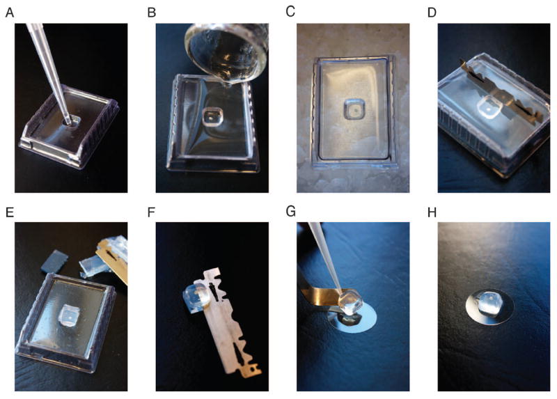
Agarose embedding of small tissue pieces or organotypic culture for two-photon imaging. (A) Transfer small tissue piece using a wide-bore 1000 μL tip in a small amount of PBS to the center of a tissue mold. (B) Carefully pour agarose solution over tissue at the corner of the mold, making certain to avoid pouring agarose directly onto the tissue. (C) Allow agarose to solidify on ice for approximately 5 minutes. (D and E) Use a sharp blade to trim excess agarose around the edges of the mold. (F) After inverting the mold and pressing the agarose-embedded tissue out, trim remaining excess agarose around and below the tissue. (G) Use a bent spatula to transfer agarose-embedded tissue onto a coverglass with a small drop of glue (see also Figure 1A and B). (H) Example of agarose-embedded tissue on cover glass ready for two-photon microscopy.

ALTERNATE PROTOCOL 2

PREPARING THYMIC SLICES FOR TWO-PHOTON IMAGING

Imaging intact thymus as described in Basic Protocol 1 allows access to the cortex since the medulla typically lies deeper than 300 μm under the capsule (Figure 3). To observe the medulla, slices that directly expose it must be used. Just as in Alternate Protocol 1, this protocol relies on embedding the organ in agarose. Similar protocols can be used for preparing tissue slices from LNs (for improved imaging of the paracortex, T cells) or spleen (for improved imaging of the white pulp versus red pulp)(Salmon et al., 2011).

Figure 3.

Two-photon microscopy of the thymus of a CD11c-YFP⁺ mouse injected with Tomato lectin–Texas Red (red) to label blood vessels, presented as a montage of maximal projections of adjacent three-dimensional data sets spanning the cut thymus from the dorsal to the ventral side. The YFP⁺ dendritic cells (yellow) are concentrated in the medulla that is surrounded by cortex.

Materials

• 4% low-melting temperature agarose in HBSS (See Reagents and Solutions)

• Molds for freezing tissue (Polysciences, Inc. catalog No. 18986-1)

• 500 mL beaker

• Crushed ice

• Sharp blade (Feather Blades: 10 pack from Leica biosystems, #39053234)

• Tissue glue (3M Vetbond tissue adhesive No. 1469SB)

• PBS

• Cover glass-18 mm circle (Fisherbrand 12-545-100 18CIR.-1)

• Vibratome (1000 Plus Sectioning System)

• Spatula (Fischer Scientific, cat # 21-401-5), bent

• 6 cm tissue culture dishes (Corning Inc, cat # 3516)

• 1Prepare 4% Agarose in HBSS. (See Reagents and Solutions)
• 2Cover with foil and put into a 37°C water bath.
• 3Harvest thymus as in Basic Protocol 1 and clean well.
• 4Fill beaker with crushed ice.
• 5Add water to ice.
• 6Fill mold halfway with agarose solution, and wait about 20 seconds before proceeding to allow agarose solution to solidify slightly.
• 7Carefully place the thymus within the agarose solution.

  • The thymus can be embedded in two orientations: horizontally to maximize the area of the thymic slice, or vertically to maximize the number of slices obtained per thymic lobe.

• 8Set mold on top of ice water mix for approximately 5 minutes or until set (Figure 4A.)
• 9Set-up the vibratome: cutting angle 5°, maximum amplitude, minimum speed.
• 10Invert the mold and gently push in the center to release the embedded tissue block (Figure 3B.)
• 11Trim the agarose with a sharp blade cut so it has slightly more agarose on the bottom of the thymus (about 0.5 cm) because the vibratome blade cannot cut below 0.5 cm above the stage (Figure 4B-4C.)
• 12Move to a dish with PBS.
• 13Put a small amount of tissue glue on the vibratome stage, and place the agarose block with embedded tissue on the drop of glue (Figure 4D.)
• 14Fill vibratome stage with cold PBS (approximately 50 mL)
• 15Cut slices to desired thickness.

  • We typically use 400 – 1000 μm thick slices. Very thin slices (<400 μm) bend and break very easily. With very thick slices, the oxygenation of the tissue becomes a concern for longer experiments.

• 16After each slice, return blade 200 μm up so that it does not drag on the cut surface.
• 17Use a bent spatula to move the slices as they are cut by the vibratome (Figure 4F.)
• 18Add a drop of tissue glue to a coverslip (Figure 1A and 1B.)

  • Using too much glue can lead to the whole organ being covered with the glue and ruining subsequent imaging steps.

• 14Use a bent spatula to transfer the sample (Figure 4H.)
• 1515. Place the agarose-embedded tissue on top of the glue on the cover glass (Figure 4H.)
• 16Immediately submerge in PBS in a 6 cm dish.
• 17Proceed to Support Protocol 1.

Figure 4.

Preparing thymic slices for direct two-photon imaging or for the introduction of exogenous cells. (A) Place the thymus or similar tissue in a tissue mold with melted agarose solution and place on ice water. (B) After inverting mold and pressing the agarose-embedded tissue out, use a sharp blade to trim excess agarose. (C) Examples of horizontally (left) or vertically (right) agarose-embedded tissue post-trimming of extra agarose. Note that there is slightly more agarose on bottom that is necessary for putting the whole tissue in the cutting range of the vibratome. (D) Agarose-embedded tissue glued to vibratome stage. (E) As the tissue slices are cut with the vibratome, use a bent spatula to transfer them out of the vibratome stage. (F) To culture and / or add cells to the tissue slice, use a bent spatula to transfer to a cell culture insert in a 6-well tissue culture dish, and carefully slide tissue slice off of spatula using a pipet tip. (G) Example of cut thymic slices on cell culture inserts where excess media has been removed. Top, horizontally embedded and sliced thymus. Bottom, vertically embedded and sliced thymus. (H) For imaging, use a bent spatula to transfer tissue slice onto coverglass that contains a small amount of glue (see also Figure 1A and B).

ALTERNATE PROTOCOL 3

OVERLAYING THYMIC SLICES WITH FLUORESCENTLY-LABELED CELLS

The introduction of thymus slices by Bhakta and Lewis opened the door for acutely introducing cell populations of choice into the three dimensional environment of the thymus and allowed researchers to circumvent time consuming chimera preparations(Bhakta and Lewis, 2005). The multitude of methods to purify cells and the availability of a range of fluorescent dyes for live cell labeling has greatly expanded the possibilities for studying thymocyte behavior. The protocol can also be applied to lymph nodes and spleen(Salmon et al., 2011).

Materials

• Thymic slices from Alternate Protocol 2, step 17

• Purified, fluorescently labeled cells of interest (e.g. CD4⁺ SP thymocytes) in media

• 6-well plates (Corning)

• 0.4 μm pore-size organotypic cell culture inserts (BD Biosciences cat. # 353090)

• Complete RPMI media (See Reagents and Solutions)

• 200 μL tip

• 200 μL pipet

1. Prepare the desired number of cell culture inserts in a 6-well plate by adding 1 ml of complete RPMI media to the bottom of the well under the cell culture insert.

2. Prepare a thymus slice as described in Alternate Protocol 2. Do not glue it to the cover glass, but instead gently put it onto a cell culture insert by pushing the slice off of a bent spatula with a pipet tip (Figure 4F.)

3. Pipet off all of the PBS surrounding the slice to prevent the cell suspension from flowing off the slice (Figure 4G.)

4. Add the single cell suspension in 10-20 μl on top of the slice.

   • We typically use 0.5-2×10⁶ cells per slice.

5. Place in the incubator.

   • We typically allow cells to migrate into the tissue for 2 hours prior to imaging.

6. Rinse tissue slices with PBS to eliminate cells that have not migrated into the tissue.

7. Add 1 mL of media to cell culture insert.

8. Add a drop of tissue glue to a coverslip (Figure 1A and 1B.)

   • Using too much glue can lead to the whole organ being covered with the glue and ruining subsequent imaging steps.

9. Using a bent spatula, transfer the sample to the coverslip that has already a small drop of tissue glue (Figure 4H.)

10. Immediately submerge in PBS in a 6 cm dish.

11. Proceed to Support Protocol 1.

SUPPORT PROTOCOL 1

SETTING UP TWO-PHOTON IMAGING CONDITIONS

Materials

• Vacuum grease (Dow Corning high vacuum grease)

• Phenol red-free DMEM (Mediatech Inc, cat # 17-205-CV)

• Oxygen (BioBlend 95% O₂, 5% CO₂ from PRAXAIR)

• 1Ensure that the temperature is controlled adequately in the imaging chamber.

  • Although lymphocytes can tolerate small deviations from 37°C, both temperature rise and temperature drop may alter cell behaviors and make them stop migrating.

• 2Ensure that the perfusion of oxygenated, phenol red-free DMEM is running at ~2 ml/min.
• 3Spread vacuum grease on the bottom of the cover glass and secure to bottom of imaging chamber.
• 4Using transmitted light, focus on the tissue sample.
• 5Switch laser to scanning mode and locate fluorescent cells or structures of interest.

  • Many organs imaged by two-photon microscopy have a capsule rich in collagen that makes a strong and easily identifiable second harmonic signal. It can be convenient to use the capsule as a position fiduciary and calculate the depth under the surface from there.

• 6Adjust the laser power and the sensitivity of the detectors for the top position (see Commentary).
• 7If there is a pre-determined depth for imaging, go to the bottom position and adjust the laser power until you reach the least power that gives acceptable image quality. If you want to image as deep as possible, survey the depth of the tissue while adjusting the laser power, and try to find the deepest point where the image quality is still acceptable. Set this as the bottom position.

  • This quick setup is inadequate for quantitative fluorescent comparisons at different depths in the tissue. It is very difficult to get quantitative fluorescence information from different depths and will certainly require standard fluorescent sources embedded in the sample.

• 7Choose appropriate number of time points, interval between time points, frame or line integration rates (See commentary).
• 8Confirm once again that all the parameters are as you desired, and ensure that the correct channels are going to be exported and saved in the correct folder.
• 9Begin imaging.

REAGENTS AND SOLUTIONS

Complete RPMI media

• Add 50 mL fetal calf serum, 5 mL of 100× Penicillin/Streptomycin solution, 5 mL100× L-Glutamine, and 0.5 mL of 1000× 2-mercaptoethanol (3.5 μl per 100 mL PBS stored at -20°C) to 450 mL RPMI 1640. Store at 4°C.

70% ethanol

• Mix together 70 mL of 100% ethanol with 30 mL of water. Store at room temperature.

4% low-melting temperature agarose in HBSS

• Add 2 g of low-melting point agarose (NuSieve GTG Agarose, Lonza, cat # 50080) per 50 mL of HBSS. Microwave on a low setting until agarose is completely dissolved (~2 min). Maintain agarose solution in 55°C water bath up to several days. Just before use (~5 min), transfer agarose solution to 37°C water bath.

COMMENTARY

Background Information

Two-photon microscopy has been used by immunologists since 2002, and it greatly expanded our ability to visualize the behavior of cells in living tissues in real time(Bousso et al., 2002; Miller et al., 2002). Prior to the introduction of this method, live imaging of immune cells in their native environment was possible only in very limited cases (e.g. cremaster muscle)(Scharffetter-Kochanek et al., 1998), and most of the studies on the immune system relied on in vitro assays or “black box” in vivo experiments. Observing the behavior of the cells in their native environment has revealed many phenomena that could not have been deduced from in vitro experiments out of tissue context. For example, in tissue culture dishes, lymphocytes are quite sessile, while in the lymph nodes they are in constant motion(Miller et al., 2002). Based on histological images, it was assumed that thymocytes are rounded cells that move little if at all, but the first two-photon imaging experiment revealed the dynamic nature of T cell development. (Bousso et al., 2002). Nowadays, two-photon imaging is routinely performed on a variety of tissues such as thymus, lymph nodes, gut, skin, liver, brain, bone marrow, etc(Bousso and Robey, 2003; Cavanagh et al., 2005; Celli et al., 2011; Chieppa et al., 2006; Egen et al., 2008; Schaeffer et al., 2009; Witt et al., 2005).

The major advantages of two-photon microscopy over other imaging methods are that it can penetrate deeper in highly scattering biological samples, it is less damaging, and there is no out of focus light. The commonly-used wavelengths for two-photon excitation (typically 700-1000 nm) lie in the near-infrared region of the spectrum where absorption and scattering from the tissue is decreased. In contrast, other microscopy methods, confocal microscopy for example, use shorter wavelength light (350-650 nm) that cannot penetrate deeper than 30-50 μm. In addition, the infrared light is less energetic than UV or visible light used in confocal microscopy and induces less photodamage. The most common type of lasers used in two-photon microscopy are femtosecond pulsed lasers that deliver short pulses of very high intensity light. Because of the pulsed nature of the laser, it delivers less total energy to the sample and is less damaging to the tissues. Finally, two-photon excitation is possible only in the very small focal volume in the sample, so no out-of-focus fluorescence is generated and all the detected light comes from a single point. However, these advantages come at a certain price. Two-photon microscopes can be very costly, with the laser being the most expensive component. In addition, the visualization of the cells or structures of interest can be difficult (see Critical parameters). Light scattering by tissues that are densely packed with cells such as the thymus and the lymph nodes decreases the fluorescent signal and makes imaging deeper than 300 μm problematic.

Critical Parameters

Modes of two-photon imaging - explants vs intravital imaging

Two-photon microscopy can be used on both explanted organs or intravitally. Both methods have advantages and disadvantages. For example, when explants are used, the blood and lymph circulation are interrupted. This is a particularly important consideration when studying homing or egress. On the other hand, the surgical trauma and use of anesthetics during intravital imaging can also complicate interpretations of imaging data. Importantly, the data on motility of lymphocytes is in very good agreement between the two methods. For some organs such as the thymus that lies in the mediastinum and is subject to large respiratory and cardiac-induced movements, explants are usually preferred. A good reference for intravital imaging is provided by Murooka and Mempel(Murooka and Mempel, 2012).

Getting the right cells labeled

A key challenge in two-photon imaging is how to fluorescently label the cells or structures of interest in a manner that preserves the integrity of the tissue. Cells can either be made to express a fluorescent protein such as green fluorescent protein (GFP) or red fluorescent protein (RFP) and their variants or be labeled ex vivo with vital dyes. Both methods have advantages and disadvantages and the method of choice depends on the particular experimental scenario.

There are a significant number of mouse models available that contain fluorescently labeled cells. Several have ubiquitously labeled cells (Ubiquitin promoter driven GFP or Actin promoter driven CFP, for example)(Hadjantonakis et al., 2002; Schaefer et al., 2001). Although not suitable for imaging directly, harvesting cell populations from these mice and re-introducing a small proportion into another mouse (bone marrow transplantation or intravenous transfer of T cells, for example) or acutely onto tissue slices is an ideal way to obtain labeled cells for imaging. In addition, there are many mouse models that express tissue or cell specific fluorescent reporters. For example CD11c-YFP in dendritic cells, LysM-GFP in phagocytic cells such as macrophages and neutrophils, or hCD2-DsRed in T cells are fluorescent reporter mice widely used for visualizing the behavior of the respective cell populations(Faust et al., 2000; Lindquist et al., 2004; Veiga-Fernandes et al., 2007). Mice expressing the recombinase Cre under the control of a suitable promoter together with a fluorescent reporter whose expression is obstructed by a floxed stop codon are very useful for fate mapping experiments(Eberl and Littman, 2004). Some, but not all, of the cell type-specific fluorescent reporters can be directly imaged within the mouse without transferring of cells from one host to another. Special attention needs to be paid to the fidelity of the cell-specific fluorescent reporters. Expression in a “wrong” cell population can easily lead to misinterpretation of the data.

Ex vivo labeling of a purified cell type (by magnetic bead enrichment or cell sorting, for example) is an ideal way to have a homogeneous population labeled if the cells can be reintroduced into tissue prior to imaging (intravenous injection or by overlaying cells on tissue slices). Vital dyes (CFSE or SNARF, for example), provide a simple and quick whole cell label suitable for two-photon imaging. Optimization of the dye’s concentration prior to imaging should be considered as the intensity will dim and will also be diluted with cell division. Ex vivo labeling of cells can also be done with calcium indicator dyes (Indo-PE3, for example). Such dyes can be powerful tools to image not only the behavior of cells, but also to monitor various modes of signaling. Another powerful, but time consuming technique for ex vivo labeling of cells is the introduction of fluorescent proteins via retroviral transduction. Here, whole cell labels or fluorescent fusion proteins can be introduced(Azar et al., 2010; Melichar et al., 2011). Although the current technology does not allow for detection of subtle movements of proteins in cells, it is adequate for quantifying large scale subcellular relocalization of proteins(Melichar et al., 2011).

Having the right number of cells per imaging volume

Having the right number of cells labeled in the imaging volume is critical for appropriate analysis of the data set. The optimal proportion of cells varies depending on the overall goal for analysis. For example, observing collective behaviors of cells (e.g. neutrophil swarming) requires higher densities of fluorescently-labeled cells than imaging and tracking of individual cells. In the latter case, for optimal results only 0.1-1% of the total cells in a given organ should be fluorescent. Sometimes, we have little control over the number of fluorescent cells in the imaging volume, especially when we deal with endogenous populations (e.g. stromal cells). However, for the cells of the immune system, there are several methods that can give appropriate number of fluorescent cells in the imaging volume. For T and B cells that naturally recirculate through the secondary lymphoid organs (spleen and LNs), intravenous injection of several million cells 6-24 h before imaging is usually sufficient for achieving optimal density of labeled cells in these organs(Henrickson et al., 2008). However, for tissues with slower turnover of immune cells (e.g brain, skin) or for highly homeostatic tissues such as the thymus, delivering the right number of fluorescent cells is not an easy task. Injected cells do not readily reach them in appreciable numbers, and therefore, bone marrow chimeras are usually required to achieve the desired density of fluorescent cells. Neonatal chimeras are generated by injecting bone marrow (BM) cells intraperitoneally into newborn mice(Ladi et al., 2008). They readily achieve a low level of chimerism (<1% donor derived cells) and are suitable when the fluorescent population derived from them is abundant. In contrast, combining fluorescent reporter expressing BM with unlabeled BM and generating mixed BM irradiation chimeras (Current Protocols in Immunology Unit 4.6) can achieve higher levels of total chimerism. There are cases in which the fluorescent protein expressing cells are less than 1% of total cells (e.g. FoxP3-GFP) and the thymus of these reporter mice can be used directly for imaging(Bettelli et al., 2006). Even if the fluorescent population is more than 1% of the total cells, but it represents a minority in a certain region (e.g. ThPOK-GFP+ cells in the cortex) the thymus of these mice can also be used directly(He et al., 2008). Generally, overlaying tissue slices with 0.5 - 2×10⁶ labeled cells (thymocyte subsets, dendritic cells, etc.), results in the appropriate density of cells for imaging. However, treatment of the sample with certain inhibitors or using cells deficient in genes that affect migration may require additional optimization. In addition, significant cell proliferation or recruitment can dramatically change the density of labeled cells in the same tissue at various time points.

Choosing the right color combinations-excitation and emission

The availability of fluorescent proteins/dyes with a wide variety of excitation and emission allows for the opportunity for combining several of them in one experiment. It is not unusual that 3 or 4 fluorophores are simultaneously used nowadays. However, this gives rise to complications such as emission spectral overlap and inefficient excitation with a single wavelength.

Emission spectral overlap is an inherent problem for all fluorescence-based methods (e.g. flow cytometry, confocal microscopy, two-photon microscopy etc.) that employ more than one fluorophore. The light emitted from each of the fluorophores is often detected in more than one channel and contributes to the fluorescence in the “wrong” channel. The usual solution is restricting the light that is detected by the photo-multiplier tubes (PMTs) by dichroic mirrors and bandpass filters. For example, we often use the following combination to separate CFP from GFP fluorescence - 495 dichroic mirror + 450/80 and 525/30 bandpass filters. This helps alleviate the problem of spectral overlap, but also decreases the brightness of the signal sometimes to unacceptable degree. An alternative solution is to use unmixing programs that determine the contribution of each fluorophore to the fluorescence detected in each channel based on single color controls, and then calculate the amount of fluorescence coming from the desired fluorophore in the respective channel. Unfortunately, such programs are not readily available for two-photon imaging and are usually custom-made by the individual investigators.

Another common problem for multicolor experiments is the necessity of excitation of several fluorophores with a single laser wavelength. Finding the optimal excitation wavelength for a multicolor experiment is mostly empirical. A starting point is to test each fluorophore individually. Frequently a literature search will turn up the two-photon optimum excitation wavelength. However, if this information is unavailable, wavelength scan can be performed. To do this:

1. Find the laser power at each wavelength that gives a good quality signal with the PMTs at their most sensitive. You must correct for the different power output of the laser at different wavelengths. The wavelength where you need the least power to get the same image is the optimum wavelength.

2. Pick the highest of the minimum output power and initially set the laser power to that wavelength.

3. With all the colors present, scan the region of the optima keeping the laser power constant. The colors will get brighter and dimmer as you pass through their respective optima. Pick the wavelength that gives the overall best image. The optimal wavelength may also vary with the relative concentration of fluorophores.

Usually some of the colors are brighter than others. In order to use the minimum laser power to image all the colors simultaneously follow these steps:

1. Start with the PMTs set to their highest sensitivity.

2. Increase the laser power slowly until you start to see fluorescence. If you still need to increase the laser power to be able to see the dimmer colors, decrease the sensitivity of the PMTs for the brighter colors.

3. Repeat until you can see all the colors adequately.

Imaging parameters

Choosing the optimal imaging parameters involves compromise between obtaining the most informative images while minimizing the damage to the sample from laser. For example, it may be desirable to image more at greater depth into the tissue, collect more closely spaced z planes and time points, and longer imaging duration. These parameters require increased exposure of the tissue to intense laser light causing damage to the tissue (photo-bleaching, photo-toxicity) and behavior change. Every investigator must decide what information is really necessary to answer the specific experimental question. The general principle is to expose the sample only to enough light to get the answer to the question. It is advisable that whenever there is a need for stronger signal, to increase the sensitivity of the detectors before increasing the laser power.

The least amount of damaging light should be used to find the sample and choose a region for imaging. To achieve this low light level imaging, the PMTs should first be set to their highest sensitivity (this maybe called voltage or gain in the controls), and the laser power should be low and slowly increased until fluorescence is detected. It may be advantageous to take snap shots of the sample instead of continuously imaging while searching for the cells and adjusting the PMT and laser power. In addition, most acquisition programs allow for averaging scanned lines or frames to increase the signal to noise ratio. However, this also increases the sample exposure to laser light. The least number of integrations that give acceptable quality should be used for continuous imaging.

As mentioned above, it is usually easier to capture the behavior of the cells of interest if they are observed for longer periods of time and with shorter intervals between time points. However, the deleterious effects of laser light (phototoxicity and photobleaching) and the scanning speed of the particular two-photon microscope impose practical limitations to this. The compromise depends on the particular experimental set up and is usually empirically determined. As a general guideline, if tracking of fast moving cells is required, the cell should not move more than one cell diameter between time points. For a cell with 8 μm diameter migrating at a speed of 16 μm/min this interval should be ~30 sec. Most often the movies are 20-60 min in duration. That is usually sufficient to capture the behavior of the cells, while avoiding bleaching of the fluorophores. However, sometimes experiments require longer periods of observation, and this necessitates making the interval between time points greater to minimize photobleaching and phototoxicity. Imaging explants beyond several hours is almost impossible because the quality of the sample deteriorates over time.

When choosing the distance between z planes, the two major considerations are the resolution limit and the size of the smallest object that needs to be reliably detected. The resolution limit is determined by the wavelength and the numeric aperture (NA) of the objective according to the formula z resolution = 2 × wavelength × refractive index medium / NA². For example if the laser is set to 920 nm and the objective has a NA 0.95, the z resolution is 2.7 μm. Thus, there is very little point setting the distance between the z planes to lower values. The size of the smallest object of interest determines the maximum distance between the z planes according to the Nyquist theorem - the frequency of sampling should be at least half of the size of that object. For example, if the cell type of interest is 8 μm, the distance between z planes should not be larger than 4 μm. For thymocytes and T cells, we typically use 3 μm spacing if we use a wavelength of 920 nm and a 20X 0.95 NA objective.

Normalizing between movies

In principal, there should be minimal variation in cell behavior from one imaging session to another under identical conditions. However, in practice, no two experiments are exactly the same and small, sometimes unnoticed changes in the conditions can have profound effects on the cells (e.g. small drop in temperature, interruption of perfusion etc.). In addition, all cell behaviors display a range of biological variation. That is why, whenever possible, it is beneficial to include a labeled, well-characterized control cell type within every imaging volume to ensure reproducibility. This is particularly useful when assessing the behavior or motility of genetically manipulated cells. Addition of differently labeled wild type cells can greatly help the interpretation of the results and avoid spending too much time pondering upon artifacts.

Software available for image analysis

A rough idea about what is happening during the movies can be obtained on the fly with the free ImageJ program. However, more detailed analysis requires the use of software packages that allow 3D visualization and automated tracking of two-photon movies, Imaris (Bitplane), Volocity (PerkinElmer) or Metamorph (Molecular Devices) for example. Even these programs often make mistakes and it is imperative that all the tracks are manually inspected to ensure that they are correct. The data from the tracking program (i.e. x, y and z positions of each tracked cell at each time point) is usually exported into Matlab (MathWorks) for automated analysis with custom written codes. The most frequently used parameters extracted from the data are average speed, speed between time points, turning angle, directionality index, arrest coefficient, and displacement. Some forms of analysis, for example frequency and duration of interaction between two cell types, are still poorly automated and require manual inspection of each track, ideally, by an unbiased individual.

Troubleshooting

No image

It is a good idea to develop a list of reasons why you are unable to get an image. The list is likely to vary with different microscopes. Here is a starting list of reasons why you may not observe an image.

1. Eye/camera mirror not in proper position

2. Inappropriate dichroic mirrors

3. PMT voltage is not on

4. Shutters are closed

5. Block or incorrect filters between dichroic mirrors and PMT

6. Laser not on

7. Transmitted or halogen light is on

8. Too much laser attenuation

9. No specimen

10. Laser alignment is incorrect

Tissue movement

It is not unreasonable to experience some tissue movement during two-photon imaging of explanted tissue. Often the tissue “settles” for a short time after being glued to the coverslip and immersed in the perfusion media. If some movement in the z plane is observed early during the imaging session, wait 5-10 minutes, and then resume imaging. If there is considerable movement in the x- and or y-dimension, check first that the tissue is glued well to the coverslip and that the coverslip is adhered well to dish. In addition, ensure that the objective is not hitting the side of the dish or the perfusion apparatus. Also, make certain that the pump speed / perfusion rate is at the proper rate. Finally, if the movement continues, check that the stage itself is not moving. Replace dish and tissue sample with a fixed sample (e.g. slide containing pollen grains), look through the eye piece and determine if the movement continues. Overall, minor tissue movement may be corrected during analysis by subtracting the apparent x,y, z motion of a fluorescent body that is know to be immotile from all coordinates at the expense of some of the data being cropped out.

Cells not moving

If the labeled cells are not moving and this is unexpected based on the experimental parameters, first ensure that warm, oxygenated media is being circulated over the explant. Next, re-visit sample preparation to ensure that no steps may have caused destruction of healthy tissue (tears of the tissue, sample out too long, wrong medium, etc.) Consider also including a labeled cell type within the image that should be unaffected under the experimental conditions (see also “Normalizing between movies” under critical parameters). Unfortunately, most of the time the reasons for the cells being immotile are unclear.

Poor quality image

Several factors can lead to an image looking “fuzzy” and the depth penetration to be unsatisfactory. First, determine if there is an issue with the perfusion or sample. Failure to clean an organ from the connective tissue or fat that surrounds it could result in poor image quality. If the liquid level is too low to cover the objective a distorted image will result. Also, if a tissue slice has been overlayed with exogenous cells, ensure that the tissue has been properly washed, as too many fluorescent cells at the top of the image may cause cells that have penetrated the tissue to look hazy, and the depth of fluorescent visibility may be poor. In addition, ensure that the objective is clean. Maintain a clean objective by cleaning thoroughly after every imaging session. Long periods of submersion in growth medium may lead to build up on the objective. Clean by submersion in water and lens cleaner. Make certain that all optical elements are properly aligned, including mirrors, lenses, dichroic mirrors, bandpass filters, detectors, etc. If any of them are off-center, fluorescence intensity and sharpness can be negatively affected. If the image appears to be “bubbling” and looks diffuse, check that the laser power is not so high that it is burning the tissue. In addition, if the fluorescence looks blurry or dimmer over time, it is possible that the fluorescent molecules are bleaching. If significant bleaching is occurring and the fluorescent marker of choice cannot be changed for future experiments, try to image using a lower laser power, take images less frequently, or shorten the length of the movie.

Anticipated Results

The anticipated results depend on the particular experimental setup. However, the usual goal is to obtain high quality movies that penetrate deep into the tissue, have clearly resolved fluorescent cells that are not too dense but with a sufficient number of cells, do not bleach and do not have tissue movement artifacts. An example of such movie is shown in Video 1.

Time Considerations

Preparation of samples for two-photon imaging

Preparing tissue (thymus, MLN, gut) for two-photon imaging of explants should take approximately 5 minutes. It is paramount to work quickly and carefully to minimize the time between sacrificing the mouse and having the intact tissue in warmed, oxygenated media or on ice. Preparing vibratome slices of tissue for two-photon imaging will reasonably take approximately 20-25 minutes in total. The melted agarose solution can be left to cool at 37°C during tissue preparation (5 min). Subsequent embedding of the tissue and solidification of the agarose (5 min), is followed by preparation of the vibratome and slicing of the tissue (5 min) prior to gluing to the coverslip. If choosing to overlay the tissue slices with fluorescently labeled cells, allow for an additional 2.5 hours. Cells are allowed to migrate into the tissue for approximately 2 hours before washing excess cells off the top of the slice. The time required for preparation of the cells to overlay on the tissue slice is not included in this estimate as this will vary significantly depending on 1) the source of the cells (single cell suspension for primary tissue vs cell culture), and 2) the labeling of the cells (ubiquitous expression of fluorescent marker, vital dye label (30 min), or Indo-PE3 (Teflabs) calcium indicator dye (2.5 hours)), for example.

Microscope set-up and imaging

Any given imaging session may take from 1.5-4 hours. The initial set-up including exchanging filter sets, warming up the laser, and initiating perfusion of the sample will generally take 5-10 min. The time required to find a suitable region for imaging (5-10 min) and time-lapse movies (20 min-1 hour) will vary considerably depending on the nature of the imaging session. In general, it is advisable to generate 3 time-lapse movies for each condition for future analysis.

Image analysis

The amount of time required to analyze one two-photon, time-lapse movie in the immune system is hugely dependent on the complexity of the image and the parameters to be analyzed. In general, tracking the migration of cells within one movie with appropriate density and bright cells that do not overlap with other fluorescently labeled cells will take approximately 2-4 hours. This includes the time it takes to load and save the data, track the migration of the cells using a program (Imaris, for example), and exporting the tracking data to a program that will calculate the parameters of interest (Matlab, for example). Analysis of other or additional parameters such as cell-cell interactions, changes in fluorescence, and morphology, will require additional time.

Supplementary Material

Supp Video S1. Videos.

Video 1: Time lapse, two-photon imaging volume of wild type GFP⁺ thymocytes in the cortex of the thymus of a mixed bone marrow chimera. The thymus was imaged as described in Basic Protocol 1. The size of the volume is 172×143×80 μm; the movie consists of 60 time points; the interval between the time points is 30 seconds.

Literature Cited

- Azar GA, Lemaitre F, Robey EA, Bousso P. Subcellular dynamics of T cell immunological synapses and kinapses in lymph nodes. Proceedings of the National Academy of Sciences of the United States of America. 2010;107:3675–80. doi: 10.1073/pnas.0905901107. [DOI] [PMC free article] [PubMed] [Google Scholar]
- Bettelli E, Carrier Y, Gao W, Korn T, Strom TB, Oukka M, Weiner HL, Kuchroo VK. Reciprocal developmental pathways for the generation of pathogenic effector TH17 and regulatory T cells. Nature. 2006;441:235–8. doi: 10.1038/nature04753. [DOI] [PubMed] [Google Scholar]
- Bhakta NR, Lewis RS. Real-time measurement of signaling and motility during T cell development in the thymus. Seminars in immunology. 2005;17:411–20. doi: 10.1016/j.smim.2005.09.004. [DOI] [PubMed] [Google Scholar]
- Bousso P, Bhakta NR, Lewis RS, Robey E. Dynamics of thymocyte-stromal cell interactions visualized by two-photon microscopy. Science. 2002;296:1876–80. doi: 10.1126/science.1070945. [DOI] [PubMed] [Google Scholar]
- Bousso P, Robey E. Dynamics of CD8+ T cell priming by dendritic cells in intact lymph nodes. Nature immunology. 2003;4:579–85. doi: 10.1038/ni928. [DOI] [PubMed] [Google Scholar]
- Cavanagh LL, Bonasio R, Mazo IB, Halin C, Cheng G, van der Velden AW, Cariappa A, Chase C, Russell P, Starnbach MN, Koni PA, Pillai S, Weninger W, von Andrian UH. Activation of bone marrow-resident memory T cells by circulating, antigen-bearing dendritic cells. Nature immunology. 2005;6:1029–37. doi: 10.1038/ni1249. [DOI] [PMC free article] [PubMed] [Google Scholar]
- Celli S, Albert ML, Bousso P. Visualizing the innate and adaptive immune responses underlying allograft rejection by two-photon microscopy. Nature medicine. 2011;17:744–9. doi: 10.1038/nm.2376. [DOI] [PubMed] [Google Scholar]
- Chieppa M, Rescigno M, Huang AY, Germain RN. Dynamic imaging of dendritic cell extension into the small bowel lumen in response to epithelial cell TLR engagement. The Journal of experimental medicine. 2006;203:2841–52. doi: 10.1084/jem.20061884. [DOI] [PMC free article] [PubMed] [Google Scholar]
- Eberl G, Littman DR. Thymic origin of intestinal alphabeta T cells revealed by fate mapping of RORgammat+ cells. Science. 2004;305:248–51. doi: 10.1126/science.1096472. [DOI] [PubMed] [Google Scholar]
- Egen JG, Rothfuchs AG, Feng CG, Winter N, Sher A, Germain RN. Macrophage and T cell dynamics during the development and disintegration of mycobacterial granulomas. Immunity. 2008;28:271–84. doi: 10.1016/j.immuni.2007.12.010. [DOI] [PMC free article] [PubMed] [Google Scholar]
- Faust N, Varas F, Kelly LM, Heck S, Graf T. Insertion of enhanced green fluorescent protein into the lysozyme gene creates mice with green fluorescent granulocytes and macrophages. Blood. 2000;96:719–26. [PubMed] [Google Scholar]
- Hadjantonakis AK, Macmaster S, Nagy A. Embryonic stem cells and mice expressing different GFP variants for multiple non-invasive reporter usage within a single animal. BMC biotechnology. 2002;2:11. doi: 10.1186/1472-6750-2-11. [DOI] [PMC free article] [PubMed] [Google Scholar]
- He X, Park K, Wang H, Zhang Y, Hua X, Li Y, Kappes DJ. CD4-CD8 lineage commitment is regulated by a silencer element at the ThPOK transcription-factor locus. Immunity. 2008;28:346–58. doi: 10.1016/j.immuni.2008.02.006. [DOI] [PubMed] [Google Scholar]
- Henrickson SE, Mempel TR, Mazo IB, Liu B, Artyomov MN, Zheng H, Peixoto A, Flynn MP, Senman B, Junt T, Wong HC, Chakraborty AK, von Andrian UH. T cell sensing of antigen dose governs interactive behavior with dendritic cells and sets a threshold for T cell activation. Nature immunology. 2008;9:282–91. doi: 10.1038/ni1559. [DOI] [PMC free article] [PubMed] [Google Scholar]
- Ladi E, Herzmark P, Robey E. In situ imaging of the mouse thymus using 2-photon microscopy. Journal of visualized experiments : JoVE. 2008 doi: 10.3791/652. [DOI] [PMC free article] [PubMed] [Google Scholar]
- Lindquist RL, Shakhar G, Dudziak D, Wardemann H, Eisenreich T, Dustin ML, Nussenzweig MC. Visualizing dendritic cell networks in vivo. Nature immunology. 2004;5:1243–50. doi: 10.1038/ni1139. [DOI] [PubMed] [Google Scholar]
- Melichar HJ, Li O, Herzmark P, Padmanabhan RK, Oliaro J, Ludford-Menting MJ, Bousso P, Russell SM, Roysam B, Robey EA. Quantifying subcellular distribution of fluorescent fusion proteins in cells migrating within tissues. Immunology and cell biology. 2011;89:549–57. doi: 10.1038/icb.2010.122. [DOI] [PubMed] [Google Scholar]
- Miller MJ, Wei SH, Parker I, Cahalan MD. Two-photon imaging of lymphocyte motility and antigen response in intact lymph node. Science. 2002;296:1869–73. doi: 10.1126/science.1070051. [DOI] [PubMed] [Google Scholar]
- Murooka TT, Mempel TR. Multiphoton intravital microscopy to study lymphocyte motility in lymph nodes. Methods in molecular biology. 2012;757:247–57. doi: 10.1007/978-1-61779-166-6_16. [DOI] [PubMed] [Google Scholar]
- Salmon H, Rivas-Caicedo A, Asperti-Boursin F, Lebugle C, Bourdoncle P, Donnadieu E. Ex vivo imaging of T cells in murine lymph node slices with widefield and confocal microscopes. Journal of visualized experiments : JoVE. 2011 doi: 10.3791/3054. [DOI] [PMC free article] [PubMed] [Google Scholar]
- Schaefer BC, Schaefer ML, Kappler JW, Marrack P, Kedl RM. Observation of antigen-dependent CD8+ T-cell/ dendritic cell interactions in vivo. Cellular immunology. 2001;214:110–22. doi: 10.1006/cimm.2001.1895. [DOI] [PubMed] [Google Scholar]
- Schaeffer M, Han SJ, Chtanova T, van Dooren GG, Herzmark P, Chen Y, Roysam B, Striepen B, Robey EA. Dynamic imaging of T cell-parasite interactions in the brains of mice chronically infected with Toxoplasma gondii. Journal of immunology. 2009;182:6379–93. doi: 10.4049/jimmunol.0804307. [DOI] [PubMed] [Google Scholar]
- Scharffetter-Kochanek K, Lu H, Norman K, van Nood N, Munoz F, Grabbe S, McArthur M, Lorenzo I, Kaplan S, Ley K, Smith CW, Montgomery CA, Rich S, Beaudet AL. Spontaneous skin ulceration and defective T cell function in CD18 null mice. The Journal of experimental medicine. 1998;188:119–31. doi: 10.1084/jem.188.1.119. [DOI] [PMC free article] [PubMed] [Google Scholar]
- Veiga-Fernandes H, Coles MC, Foster KE, Patel A, Williams A, Natarajan D, Barlow A, Pachnis V, Kioussis D. Tyrosine kinase receptor RET is a key regulator of Peyer’s patch organogenesis. Nature. 2007;446:547–51. doi: 10.1038/nature05597. [DOI] [PubMed] [Google Scholar]
- Witt CM, Raychaudhuri S, Schaefer B, Chakraborty AK, Robey EA. Directed migration of positively selected thymocytes visualized in real time. PLoS biology. 2005;3:e160. doi: 10.1371/journal.pbio.0030160. [DOI] [PMC free article] [PubMed] [Google Scholar]
Associated Data
This section collects any data citations, data availability statements, or supplementary materials included in this article.
Supplementary Materials