Experimental demonstration of novel imaging geometries for x-ray fluorescence computed tomography

Abstract

Purpose: X-ray fluorescence computed tomography (XFCT) is an emerging imaging modality that maps the three-dimensional distribution of elements, generally metals, in ex vivo specimens and potentially in living animals and humans. At present, it is generally performed at synchrotrons, taking advantage of the high flux of monochromatic x rays, but recent work has demonstrated the feasibility of using laboratory-based x-ray tube sources. In this paper, the authors report the development and experimental implementation of two novel imaging geometries for mapping of trace metals in biological samples with ∼50–500 μm spatial resolution.

Methods: One of the new imaging approaches involves illuminating and scanning a single slice of the object and imaging each slice's x-ray fluorescent emissions using a position-sensitive detector and a pinhole collimator. The other involves illuminating a single line through the object and imaging the emissions using a position-sensitive detector and a slit collimator. They have implemented both of these using synchrotron radiation at the Advanced Photon Source.

Results: The authors show that it is possible to achieve 250 eV energy resolution using an electron multiplying CCD operating in a quasiphoton-counting mode. Doing so allowed them to generate elemental images using both of the novel geometries for imaging of phantoms and, for the second geometry, an osmium-stained zebrafish.

Conclusions: The authors have demonstrated the feasibility of these two novel approaches to XFCT imaging. While they use synchrotron radiation in this demonstration, the geometries could readily be translated to laboratory systems based on tube sources.

INTRODUCTION

Background and significance

X-ray fluorescence computed tomography (XFCT) is an emerging imaging modality that maps the three-dimensional (3D) distribution of elements, generally metals, in ex vivo specimens and potentially in living animals and humans. Many endogenous metals and metal ions, such as Fe, Cu, and Zn, play critical roles in signal transduction and reaction catalysis, while others (Hg, Cd, Pb) are quite toxic even in trace quantities.¹ In the postgenomic era, the new disciplines of metallogenomics, metalloproteomics, and metallomics are emerging for the systematic study of endogenous metals.^{1, 2, 3} These disciplines would benefit greatly from the spatially resolved maps of trace-element distribution provided by XFCT.^{1, 2, 3}

In addition, exogenous metals are often critical components of new in vivo molecular imaging agents: Gd and Mn are used in magnetic resonance imaging agents, and Cd and Au are used in nanoparticle-based optical imaging agents.^{4, 5, 6, 7, 8, 9, 10, 11, 12, 13} When applied to tissue samples excised from animal models, for instance, XFCT techniques could provide calibration and subcellular localization information critical for the continued advancement of these technologies.¹⁴

History and current approaches to XFCT

XFCT is an induced-emission method in which an external source of x rays is used to stimulate emission of characteristic x rays from a sample, and it has the ability to produce three-dimensional maps of the distribution of individual elements in a small, intact specimen. It can map such elements simultaneously, in trace (parts per million) quantities, and at high resolution.

XFCT was first proposed by Boisseau^{15, 16} in 1986, and the technique's biological potential was immediately apparent, as he applied the technique to imaging the distribution of iron and titanium in the head of a bee. Synchrotron-based XFCT is most commonly performed in a first-generation tomographic geometry, acquiring a single line integral at a time as depicted in Fig. 1. A pencil beam of x rays illuminates a selected line through the sample. In third-generation synchrotrons such as the Advanced Photon Source, the beam width can be as small as a few micrometers and still deliver 10¹⁰ monochromatic photons per second. As the beam travels through the object, it undergoes photoelectric interactions with inner-shell electrons of atoms in the sample; these atoms, in turn, emit isotropically distributed characteristic x rays that can be detected by the energy-sensitive (but not position-sensitive) fluorescence detector.

Figure 1.

Standard line-by-line scanning method. A pencil beam illuminates a line through the object, stimulating emission of characteristic x-rays that are detected by an uncollimated, nonposition sensitive detector. The object must be translated and rotated in order to build up a sinogram. This figure is reprinted with permission from Meng et al., “X-ray fluorescence tomography using emission tomography systems,” IEEE Trans. Nucl. Sci. 58, 3359–3369 (2011). Copyright © 2011, IEEE.

Historically, dwell times per line-integral measurement have been on the order of 0.5–1.5 s. The object is then scanned through the beam, line by line, and then rotated, as the line-by-line scan of the object must be repeated at dozens of projection views over 180° or 360° to obtain the data necessary for image reconstruction.¹⁷ The entire process typically took well over an hour for a single slice through a typical sample. Recently, significant efforts have been made to improve the speed of the first-generation acquisition, including the use of faster detectors and continuous “fly” scanning procedures that eliminate deadtime.^{18, 19} These allow for line integral acquisition times on the order of 3 ms and have reduced per slice acquisition times to the point that isotropic three-dimensional stacks can be acquired in a few hours.

In the absence of attenuation, the height of each spectral peak acquired for a given illumination line would correspond to the line integral through the corresponding element's distribution along that line. The scanning and rotation would provide samples of the Radon transform of the elemental distributions. The Radon transform is the well-known line integral mapping that underlies medical CT, and it can be readily inverted by simple algorithms such as filtered backprojection (FBP). Unfortunately, attenuation is significant in XFCT and the data are not well modeled as the Radon transform of the elemental distributions. A few algorithms that address the attenuation problem have been described in the literature;^{20, 21, 22, 23, 24} we have developed two novel penalized-likelihood approaches that match or exceed the performance of these earlier algorithms.^{25, 26}

It is worth making clear that the attenuation of the characteristic x rays limits the size of the sample that can be imaged for a given element of interest or, conversely, that determines the set of accessible elements for a sample of a given size. Calcium K_α emissions are at 3.691 keV, which has a mean free path (MFP), 1/μ, of only 0.1 mm in a tissue background, while zinc K_α emissions are at 8.639 keV, which has a MFP of 1.0 mm in tissue. In terms of mapping a wide range of metals, the technique is thus best suited for ex vivo imaging of subcentimeter specimens. In vivo imaging may be possible for heavier metals, either endogenous or exogenously introduced contrast agents. Gold K_α emissions, for example, are at 68.803 keV, and have a MFP of 5.1 cm in tissue. Recent simulation and experimental work by the groups of Cho^{27, 28, 29} and Xing³⁰ have demonstrated the feasibility of using XFCT to detect gold nanoparticles in vivo at reasonable radiation doses.

The groups pursuing in vivo implementations of XFCT have explored the use of new geometries that offer improvements over the first generation geometry in regimes where micrometer-scale resolution is not required. Huo et al.³¹ used a sheet beam to illuminate an entire slice at once and placed a 1D array of collimated detectors at 90° to the beam. The array of detectors thus acquired a parallel-beam projection of the fluorescence emission. The object was rotated to acquire a full set of such projections, which could be used for tomographic reconstruction. The group of Cho^{28, 29} demonstrated benchtop XFCT using a tube source both experimentally and computationally. They illuminated the entire object and scanned an opposing pair of single-element collimated detectors to acquire each projection. The sample was then rotated and the process repeated to acquire additional views. They note that the use of a 1D array of collimated detectors, as in Huo³¹ above, would eliminate the need for scanning and that a 2D collimated array would allow for simultaneous multislice acquisition.

Recently, we have been exploring the possibility of speeding acquisition in XFCT by using novel detection systems based on position-sensitive x-ray detectors and collimating apertures, as is done in single-photon emission tomography.³² This was motivated by several recent developments. First, position sensitive x-ray spectrometers with sufficient detection area, adequate energy resolution (a few hundred eV), excellent spatial resolution (a few tens of micrometers), and reasonable cost-effectiveness have become available. Second, recent developments of single photon emission microscope systems have offered an improved understanding on the design of microcollimation methods that offer reasonable detection efficiency at excellent spatial resolution.³³

We are considering two novel geometries, illustrated schematically in Fig. 2. In the first, shown on the left, a plane-collimated sheet of x rays illuminates a single slice through the object, inducing emission of characteristic x rays. A position- and energy-sensitive detector collimated by one or more pinholes images these emissions, recording an x-ray spectrum in each pixel. Neglecting attenuation and other physical effects, the resulting image for each spectral emission peak will be a direct image of the distribution of the element associated with that peak. In practice, it will be necessary to account for attenuation and geometric obliquity effects, but the basic concept entails a direct selective-plane acquisition.

Figure 2.

Schematic illustration of the implemented imaging approaches. (a) A sheet beam of x-rays illuminates a single plane through the object and the resulting emissions are imaged through a pinhole. This produces a direct image of the plane of interest. Scanning the object through the plane allows formation of a 3D image. (b) A pencil beam of x-rays illuminates a line through the object and the emissions are imaged through a slit collimator. In this case, the acquired image is collapsed along the column direction (vertically) in order to obtain a direct image of the illuminated line. Scanning the object through the line allows formation of a 3D image. While this approach involves more object motion, the sensitivity of the slit collimator is much larger than that of the pinhole.

In the second geometry, a pencil beam of radiation illuminates a line through the object, inducing emission of characteristic x rays from along that line. These emissions are imaged by a position- and energy-sensitive detector collimated by one or more slit collimators. The emissions from a given point along the line project through the slit and illuminate an entire column of the detector. Neglecting attenuation and obliquity effects, the acquired image at each emission peak can be collapsed along the column direction to obtain the element distribution along the illuminated line.

An extensive Monte Carlo study has shown that both geometries potentially offer advantages over the current line-by-line approach.³² We found that pencil beam illumination combined with the slit collimator could provide an order-of-magnitude improvement in imaging speed without increasing radiation dose rate when compared to a line-by-line approach using a detector with 5% overall detection efficiency. The use of slit-apertures also offers reasonable detection efficiency, even with very fine slit widths (down to a few micrometers). This makes it well suited for rapid, high-resolution XFCT imaging studies. The combination of sheet illumination with pinhole collimators was found to achieve a much higher imaging speed by allowing synchrotron x rays to irradiate an extended volume of the object. This helps to offset the low efficiency of the pinhole detection system. However, the improvement in imaging speed is attained at the cost of a much greater dose-rate to the object and this imaging mode is less suitable for high-resolution XFCT studies because of the challenges of fabricating micrometer-scale pinholes and their extremely low sensitivity.

In this work, we show the first experimental demonstration of these two novel geometries. The limited synchrotron beamtime and the use of two different borrowed detectors did not allow for systematic comparison of the methods with each other or with the first-generation approach but did allow sufficient time to demonstrate the feasibility and promise of the approaches.

We considered exploring a third geometry, in which the pinhole detection geometry is combined with illumination of the entire object. In this case, the entire object isotropically emits fluorescence x rays, and the camera acquires pinhole projection images that can be used to solve for the elemental densities through an inverse problem similar to that arising in pinhole SPECT. This geometry has been explored in conjunction with illumination by an x-ray tube by Bruyndonckx et al.³⁴ and incorporated into a specimen micro-CT system (SkyScan 2140, Bruker, Inc.). However, Monte Carlo simulations we performed showed that this was not competitive with the two geometries we explore here in the context of high-flux synchrotron imaging, so we did not pursue that geometry in this study.

METHODS

Planar illumination with pinhole detection aperture

The experimental setup used in the feasibility study of the pinhole geometry is shown in Fig. 3. The detection system consisted of a single front-illuminated x-ray CCD detector on loan from Andor Technology (Model # 934N). It had a detection area of 2.56 × 1.52 cm, with 1280 × 768 square pixels of 20 × 20 μm in size. The detection efficiency of the detector is ∼80% at 5 keV, ∼30% at 10 keV, and ∼15% at 15 keV. The space around the CCD sensor was filled with dry hydrogen and the sensor was cooled to −15 °C to reduce dark noise. X-ray interactions were identified with a photon-counting algorithm that was previously described in Ref. 35. This process offers an energy resolution of ∼250 keV FWHM.

Figure 3.

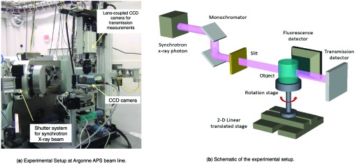
The experimental setup for the preliminary pinhole XFCT study: (a) experimental setup at Argonne APS beam line, (b) schematic of the experimental setup. The detection system consists of an X-ray CCD detector and a multiple pinhole aperture. The translation stage was used to perform a 1D translation of the object through the sheet beam. The rotation stage was used only during the separate process of acquiring a standard transmission CT for attenuation correction.

In this study, we used synchrotron x rays of 15 keV to irradiate the sample. The beam profile was modulated with a PC-controlled aperture that can provide a thin, vertical sheet-like parallel beam (we used 50 μm width × 5 mm height). The beam intensity was fixed at ∼10¹¹ photons per second per cm². An x-ray shutter was installed on the beam line, and its operation was synchronized with the readout of the CCD to eliminate any smearing effect. In this study, the CCD was typically operated with 1–5 s accumulation time per frame followed by a readout period of 1 s. We accumulated and averaged frames for a total imaging time of 5 min per slice.

We tested a multiple-pinhole aperture with 3 × 5 pinholes of 300 μm diameter and an interpinhole distance of 3 mm. It was fabricated with tungsten sheets of 500 μm thickness. The pinholes had cone-shaped profiles on both sides, with a fixed acceptance-angle of 45°. The detector-to-aperture distance was 1.5 mm and the center of the object was 1.2 mm from the aperture.

To determine the system response function, a lead ball with diameter approximately 400 μm was used to calibrate the detection system. The lead ball was directly scanned with 2D movement in the beam plane with a fixed step size (typically 500 μm). The ball was then translated along vertical direction (almost parallel to the beam profile) and the measurement was repeated at several different heights according to FOV. The resulting set of data was used to estimate the geometric and sensitivity parameters of the system using least-squares fitting based on the Levenburg-Marquardt algorithm.

The phantom used in this experimental study consisted of three plastic tubes of 0.75 mm inner diameter. These tubes were filled with uniform solutions containing 25 mM Fe, 50 mM Zn, and 25 mM Br, respectively. A larger plastic tube was used to hold the three tubes together. Its inner diameter was around 12 mm. We stepped the object through the sheet-beam in 50 μm steps. The results of this experiment are presented in Sec. 3A.

Pencil beam illumination with slit collimation

For the second experiment, conducted in a separate beamtime run, we employed a back-illuminated x-ray CCD detector (Andor Technology: ikon-L936DO), which is specifically designed for direct x-ray detection with high spatial resolution. The 2048 × 2048 pixels and 13.5 μm pixel size combine to offer a 2.76 × 2.76 cm active image area. A large area five-stage TE cooler enables cooling of this large sensor down to −30 °C with air cooling. The detection efficiency is ∼60% at 5 keV and ∼15% at 10 keV. We employed a single slit aperture of width 50 μm. The slit opening was fabricated with an acceptance angle of 75° in the plane perpendicular to the central line through the slit. In the experiment, the beam-to-slit distance was about 7.5 mm with the magnification factor of ∼3. The geometry is depicted in Fig. 4. Note that the object was inadvertently not perfectly centered on the slit, though the obliqueness is exaggerated in the figure, which is not to scale.

Figure 4.

Geometry for the pencil beam illumination and slit collimation geometry.

We imaged two different objects. The first was a tube phantom made of three capillary tubes (ID: 550 μm and OD: 800 μm), which were filled with NaBr (Br: 9.8 mg/ml), CuCl₂ (Cu: 12 mg/ml), and water, respectively. The second object imaged was a 5 day-postfertilization zebrafish embryo that was sacrificed, fixed, and stained with 1% Osmium Tetroxide prior to embedding in Embed-812, a resin frequently used in electron microscopy. The sample was prepared previously for high-resolution micro-CT phenotyping of zebrafish, which have become important biological model organisms. For both objects, a pencil beam of 50 × 50 μm in size was used, while the object was scanned line-by-line with a fixed step size of 50 μm. A 40-s data acquisition was used at each step. Following the fluorescence measurements, we also acquired a standard transmission CT scan of the phantoms at 15 keV, which will aid in performing attenuation correction. These CT scans were reconstructed on a 400 × 400 × 439 grid of 11.4 μm pixels.

Dose estimation

To get a sense of the radiation dose delivered to the objects, we use the beam flux parameters to perform a simple analytic calculation of the dose delivered at a depth of 2 mm in tissue. We calculate the dose as

$$D=\psi \left({\mu }_{\mathrm{en}}/\rho \right),$$

where ψ is the primary photon fluence in J/cm² and (μ_en/ρ) is the mass energy absorption coefficient of the tissue at the incident beam energy 15 keV, which is 1.4 cm²/g. The primary photon fluence is given by

$$\psi =k{I}_{0}Et\exp (-\mu z),$$

where k = 1.8 × 10⁻¹⁶ J/keV is a conversion factor, I₀ = 10¹¹ photons s⁻¹ cm⁻² is the incident photon flux density, t = 40 s is the dwell time, μ = 1.7 cm⁻¹ is the linear attenuation coefficient in tissue at 15 keV, and z = 0.2 cm is the depth at which we are computing the dose. Evaluating this expression yields a dose of 9.25 Gy. While this dose is obviously too high for in vivo imaging, such imaging would not likely be carried out at 50 μm spatial resolution. In the results presented here, 0.2 g/cm³ concentrations of osmium are readily detected in 50 μm resolution elements, which corresponds to 25 ng of heavy metal per resolution element. In vivo applications have typically sought to detect on the order of 1 mg per resolution element.²⁹ A substantial dose reduction could be achieved by working at similarly reduced resolution.

RESULTS

Planar illumination with pinhole detection aperture

A typical energy spectrum measured with the CCD sensor is shown in Fig. 5. The FWHM value around the Br photopeak was around 250 eV, which allows us to resolve the x-ray lines from the three trace elements. The area under the three elemental peaks of interest was calculated at each pixel in the CCD allowing formation of element-specific pinhole images. An image obtained by the CCD upon illumination of the central slice of the phantom is shown in the left panel of Fig. 6, where green pixels denote zinc and blue pixels bromine (the iron-containing tube did not intersect this slice). Fifteen replicate images can be seen corresponding to the 15 pinholes. A single image was synthesized from the 15 pinhole images, accounting for geometric obliquity effects, by use of the MLEM algorithm, as shown in the central panel of Fig. 6. The resulting slice was then appropriately placed into a 3D stack, as shown in the right panel.

Figure 5.

Energy spectrum measured with the x-ray CCD detector. The energy threshold used for selecting fluorescence components are shown in the figure.

Figure 6.

Illustration of the data acquisition and image formation process for the pinhole geometry. The blue color denotes bromine and the green color zinc. This represents data acquired during illumination of the central slice of the phantom.

Figure 7 shows three surface renderings, from three different angular positions, of the full 3D reconstruction, where the three entwined tubes can be seen. These results demonstrate the feasibility of the proposed emission tomography detection approach, which is seen to have sufficient energy and spatial resolution to distinguish and spatially resolve the distribution of the three elements.

Figure 7.

Three views of a 3D rendering of the reconstructed elemental distribution with data acquired in the pinhole geometry. (Red = iron, green = zinc, blue = bromine).

Pencil beam illumination with slit collimation

Each illumination line produced a full spectrum at each pixel in the CCD. The photon count numbers under the bromine, copper, and Compton scatter peaks were calculated for the tube phantom and likewise under the osmium peak for the zebrafish data. The resulting images were collapsed along the column direction to yield the initial estimate of elemental concentration along the illumination line. These lines were then assembled into a three-dimensional image estimate.

For the tube data, the reconstructed photon count data sets were upsampled from 50 μm voxels to 11.4 μm voxels using trilinear interpolation to match the voxel size and dimensions of the transmission attenuation data sets. These data sets were then registered using 3D vector-based rigid body registration. The density of copper and bromine present were estimated based on the following model:

$$\begin{array}{ccc}\hfill y_{\mathrm{pix}}^{\mathrm{elem}}& =& \left[I_{0}At{F}_{\mathrm{pix}}\left({\vec{\mu }}_{\mathrm{inc}}\right)\right]\left[{\left(\frac{\tau }{\rho }\right)}_{\mathrm{elem}}{p}_k{\rho }_{\mathrm{elem}}\Delta x{\omega }_k\upsilon \alpha \right]\hfill \\ & & \times \left[\varepsilon \Omega G_{\mathrm{Pix}}\left({\vec{\mu }}_{\mathrm{Fluoro}}\right)\right].\hfill \end{array}$$

The goal is, of course, to solve for ρ_elem. The quantities in this equation are defined in Table 1. The terms in the first square bracket pair represent the number of incident photons that reach the pixel of interest. The terms in the second square bracket pair represent the fraction of those photons that are absorbed and lead to emission of a characteristic x ray corresponding to the emission line that will be captured in the spectral emission peak. The terms in the third square bracket pair represent the fraction of those characteristic x rays that are actually detected, having survived attenuation in the object and successfully passed through the slit and interacted in the detector.

Table 1.

Model parameters.

Quantity	Definition	Units	Value for Br	Value for Cu
$y_{\mathrm{pix}}^{\mathrm{elem}}$	Detected number of photons in pixel for element of interest	Number	NA: Measured quantity	NA: Measured quantity
I0	Incident photon flux density	Number s−1 cm−2	1011	1011
A	Beam area	cm2	2.5 × 10−5	2.5 × 10−5
t	Dwell time	s	40	40
$F_{\mathrm{Pix}}\left({\vec{\mu }}_{\mathrm{inc}}\right)$	Fraction of incident photons that reach pixel of interest without being attenuated	Dimensionless	Calculated from measured attenuation map at beam energy	Calculated from measured attenuation map at beam energy
${\left(\frac{\tau }{\rho }\right)}_{\mathrm{elem}}$	Photoelectric cross section	cm2/g	111.0	73.1
pk	Fraction of photoelectric interactions with K shell	Dimensionless	0.856	0.874
ρelem	Density of element	g/cm3	NA: Quantity being estimated	NA: Quantity being estimated
Δx	Voxel size	cm	0.005	0.005
ωκ	Fluorescence yield of k shell	Dimensionless	0.618	0.439
να	Branching ratio of detected line(s)	Dimensionless	0.91	1.00
$G\left({\vec{\mu }}_{\mathrm{Fluoro}}\right)$	Fraction of emitted x-rays that reach slit opening without being attenuated	Dimensionless	Calculated from measured attenuation map at beam energy (see text)	Calculated from measured attenuation map at beam energy (see text)
ɛ	Detector efficiency at emission energy	Dimensionless	0.10	0.23
Ω	Geometric efficiency	Dimensionless	0.0005	0.0005

The two attenuation terms bear further comment. The first, $F_{\mathrm{pix}}\left({\vec{\mu }}_{\mathrm{inc}}\right)$, denotes the fraction of incident photons that reach the pixel of interest without being attenuated. This is very straightforward to calculate from the transmission CT scan since it provides the attenuation coefficients at the incident beam energy. The second, $G\left({\vec{\mu }}_{\mathrm{Fluoro}}\right)$, denotes the fraction of emitted characteristic x rays, traveling along the path between the pixel and the slit, that escape the object without being attenuated. Estimating this term is more subtle because it requires knowledge of the attenuation map at the emission energies of bromine (11.9 keV) and copper (8.0 keV), while we have measured it only at the incident beam energy (15 keV). To first order, we can estimate the attenuation map at these energies by scaling the measured attenuation map by the classic photoelectric energy dependence (E_inc/E_fluoro)ⁿ, where n∼3 (we use n = 2.83 based on the model of Leroux³⁶). However, this simple correction neglects the fact that the emissions of each element are necessarily below the element's own K edge and so the simple photoelectric scaling overestimates the attenuation coefficient. The attenuation map at the lower energies should be adjusted based on the distributions of the elements themselves, which are the very quantities being estimated. We deal with this situation through a recursive correction, similar to one we have used previously in the context of fully iterative reconstruction for first-generation XFCT.^{25, 26} In short, the attenuation map estimates are recursively improved by incorporating the latest estimate of the density map, again based on Leroux's parametrization. To minimize artifacts, the density map estimates used were thresholded. Density values below 2 orders of magnitude of the expected densities are assumed to be noise and set to 0. Additionally, density values greater than 1 order of magnitude of the expected values are assumed to be scatter and are also set to 0.

Cross-sectional images and average radial profiles tube reconstructions from the slit collimation geometry are shown in Figs. 89 for bromine and copper, respectively. The average density values calculated in the tubes are reported in Table 2. A 3D rendering of the full set of reconstructed slices is shown in Fig. 10. For bromine, the calibration and correction procedure recovers fairly accurate average concentration values, although there is a residual artifact in the final image that is probably attributable to imperfections in the attenuation correction procedure (the shadow through the tube corresponds to pixels whose emissions pass through the glass portion of the copper-containing tube). The reconstruction of the copper containing tube is much more uniform, although the recovered values are approximately double the true values. This may also be attributable to inaccuracies in the attenuation correction procedure. Since the copper emission energy is the lower of the two, it is subject to higher attenuation and is more sensitive to inaccuracies in estimation of the attenuation map. Indeed, the Leroux model tends to result in ∼35% overestimate of attenuation at the copper energy. We are currently investigating improved methods of attenuation estimation and correction for these geometries.

Figure 8.

(Left) Typical uncorrected and attenuation-corrected slices through the bromine containing tube. (Right) Average radial profile through the slice showing that the attenuation correction procedure improves quantitative accuracy albeit at the expense of boosting the nonuniformity of the reconstructed profile.

Figure 9.

(Left) Typical uncorrected and attenuation-corrected slices through the copper containing tube. (Right) Average radial profile through the slice. In this case, the attenuation correction procedure leads to an overestimate of the true copper concentration.

Table 2.

Average elemental concentrations calculated in tube lumen.

Element	True density (mg/cm3)	Initial estimate (mg/cm3)	With correction (mg/cm3)
Bromine	12.0	5.3	9.3
Copper	9.8	6.9	20.3

Figure 10.

Three-dimensional rendering of the reconstructed elemental distributions (near tube = copper, central tube = bromine) overlaid on a reconstruction of the signal from the Compton scatter peak which shows the outline of the glass tubes. Note that the most distant tube contained only water.

The results for the osmium-stained zebrafish are shown in Fig. 11. It can be seen that prior to attenuation correction, there is a clear gradient of apparent osmium density across the fish, where we would expect more symmetric staining. Such symmetry is restored by the correction procedure. To check for quantitative accuracy, we computed the average density of osmium in the lens of the eye and found it to be 0.25 ± 0.05 g/cm³. This is consistent with previous work we had done in zebrafish using micro-CT, where L-edge subtraction for osmium yielded values around 0.22 ± 0.03 g/cm³.

Figure 11.

Uncorrected and corrected axial and sagittal slices from the osmium stained zebrafish. The average density of osmium in the lens of the eye is 0.25 ± 0.05 g/cm³ in the corrected images. This is consistent with previous values we have found in stained zebrafish using micro-CT, where L-edge subtraction for osmium yielded values around 0.22 ± 0.03 g/cm³.

DISCUSSION AND CONCLUSIONS

We have demonstrated the implementation of two novel approaches to three-dimensional x-ray fluorescence imaging. One involves illuminating a single plane through the object and using a pinhole-collimated detector to form an image of the emissions from that plane and the other involves illuminating a single line through the object and using a slit-collimated detector. As implemented, each approach used a single imaging detector. In principle, additional detectors could be used to surround the object, as depicted in Fig. 12. Moreover, the collimators can contain multiple pinholes (as was the case here) or multiple slits, respectively, in order to use the imaging sensor as fully as possible. The simplest implementation would space the pinholes or slits so as to avoid any overlapping of the images from each collimator opening, but some multiplexing could be tolerated.

Figure 12.

Potential higher-sensitivity implementations of the proposed geometries using (a) multiple pinholes illuminating multiple detectors and (b) multiple slits illuminating multiple detectors. This figure is reprinted with permission from Meng et al., “X-ray fluorescence tomography using emission tomography systems,” IEEE Trans. Nucl. Sci. 58, 3359–3369 (2011). Copyright © 2011, IEEE.

The reason these novel geometries offer some potential advantage over the existing first-generation approach lies in exploiting the combination of selective illumination and position-sensitive detection to eliminate the need for solving a full inverse problem. Consider, for example, the tradeoffs involved in the pinhole geometry and the first-generation tomography approach. With the pinhole, one acquires an entire image directly in one illumination while the first-generation approach involves line-by-line acquisition of a sinogram. However, the direct image is acquired through a pinhole collimator that rejects most of the characteristic x rays whereas the sinogram is acquired with an uncollimated detector. One might expect these two effects to cancel, leading to equal total imaging time for a given signal-to-noise ratio. But this is not the case. The key difference is that, all else being equal, an image is preferable to a sinogram because to obtain an image from a sinogram, one must solve an inverse problem that inevitably amplifies data noise. We have analyzed this tradeoff in more detail in a previous publication.³⁷ The pencil beam illumination with slit collimation represents a more optimal middle ground, offering much higher sensitivity than the pinhole collimation strategy while still avoiding the need to solve an inverse problem. These considerations also explain why the third potential geometry discussed in the Introduction, illumination of the entire object combined with pinhole-collimated detectors, was found to be a poor choice in our previous Monte Carlo studies. This SPECT-like setup leads to solution of an ill-posed inverse problem because it does not exploit the ability to selectively induce emission of x rays through controlled illumination.

One potential drawback of the new geometries is the challenge of attenuation correction, since the attenuation correction at a given point depends on properly correcting for errors in the regions between it and both the source and detector. This accumulation of errors tends to create high uncertainty in the regions of the object that are far from both the source and detector. This could potentially be mitigated by alternative, attenuation-minimizing acquisitions, such as rotating the object by 180° after acquiring the direct measurements for the half of the object closest to the detector or even performing an “onion peeling” acquisition in which a combination of rotational and translational sample motion are deployed such that the direct measurements are made along concentric radial shells so as to minimize attenuation. These remain subjects for future investigation.

It is worth making clear that the new geometries cannot at present challenge the existing first-generation geometry in the realm of maximum achievable spatial resolution. The first-generation geometry resolution is determined entirely by the size of the pencil beam, which at a synchrotron can be submicrometer and still retain reasonable flux. In the pinhole geometry, the resolution is determined mainly by the size of the pinholes and the magnification geometry and can likely not be better than 10 μm because of fabrication limitations and sensitivity constraints. The slit geometry resolution is determined by the size of the pencil beam in the axial plane and by the size of the slit and magnification geometry along the depth axis. It is possible to fabricate slits on the order of 5 μm.

One can imagine using these approaches in the synchrotron context to somewhat rapidly survey entire objects at 10–50 μm resolution in order to identify specimens or regions of interest (ROI) for further study at higher resolution. It is worth noting that these approaches very naturally lend themselves to region of interest imaging, since one can restrict attention to certain planes or lines through the object, whereas the first generation approach generally requires acquisition of a complete sinogram in order to achieve stable reconstruction, although there is some limited data acquisition reduction possible when imaging a ROI tomographically.³⁸

Finally, these approaches are very well suited to translation into benchtop systems employing tube sources. Such sources have insufficient flux to achieve micrometer or submicrometer resolution imaging in a first-generation geometry and are thus well suited for use in this 10–500 μm resolution regime. The main challenges introduced by tube sources are longer imaging times and the polychromatic spectrum. Longer imaging times are not necessarily a issue for ex vivo specimens and are largely offset by improved access relative to synchrotrons. The polychromatic spectrum introduces challenges in the form of Compton scatter photons of a variety of energies contaminating the acquired spectrum, where monochromatic synchrotron studies usually have a fairly well-defined Compton scatter peak that can be isolated from the emission peaks by judicious choice of beam energy. This issue can be mitigated through careful beam filtering, kVp selection, and spectral modeling.

References

- Lobinski R., Moulin C., and Ortega R., “Imaging and speciation of trace elements in biological environment,” Biochimie 88, 1591–1604 (2006). 10.1016/j.biochi.2006.10.003 [DOI] [PubMed] [Google Scholar]
- Paunesku T., Vogt S., Maser J., Lai B., and Woloschak G., “X-ray fluorescence microprobe imaging in biology and medicine,” J. Cell. Biochem. 99, 1489–1502 (2006). 10.1002/jcb.21047 [DOI] [PubMed] [Google Scholar]
- Fahrni C. J., “Biological applications of X-ray fluorescence microscopy: Exploring the subcellular topography and speciation of transition metals,” Curr. Opin. Chem. Biol. 11, 121–127 (2007). 10.1016/j.cbpa.2007.02.039 [DOI] [PubMed] [Google Scholar]
- Caravan P., Ellison J. J., McMurry T. J., and Lauffer R. B., “Gadolinium(III) chelates as MRI contrast agents: Structure, dynamics, and applications,” Chem. Rev. 99, 2293–2353 (1999). 10.1021/cr980440x [DOI] [PubMed] [Google Scholar]
- Gao X., Cui Y., Levenson R. M., Chung L. W. K., and Nie S., “In vivo cancer targeting and imaging with semiconductor quantum dots,” Nat. Biotechnol. 22, 969–976 (2004). 10.1038/nbt994 [DOI] [PubMed] [Google Scholar]
- Miller L. M., Wang Q., Telivala T. P., Smith R. J., Lanzirotti A., and Miklossy J., “Synchrotron-based infrared and X-ray imaging shows focalized accumulation of Cu and Zn co-localized with β-amyloid deposits in Alzheimer's disease,” J. Struct. Biol. 155, 30–37 (2006). 10.1016/j.jsb.2005.09.004 [DOI] [PubMed] [Google Scholar]
- Tomik B., Chwiej J., Szczerbowska-Boruchowska M., Lankosz M., Wojcik S., Adamek D., Falkenberg G., Bohic S., Simionovici A., Stegowski Z., and Szczudlik A., “Implementation of X-ray fluorescence microscopy for investigation of elemental abnormalities in amyotrophic lateral sclerosis,” Neurochem. Res. 31, 321–331 (2006). 10.1007/s11064-005-9030-6 [DOI] [PubMed] [Google Scholar]
- Finney L., Mandava S., Ursos L., Zhang W., Rodi D., Vogt S., Legnini D., Maser J., Ikpatt F., Olopade O. I., and Glesne D., “X-ray fluorescence microscopy reveals large-scale relocalization and extracellular translocation of cellular copper during angiogenesis,” Proc. Natl. Acad. Sci. U.S.A. 104, 2247–2252 (2007). 10.1073/pnas.0607238104 [DOI] [PMC free article] [PubMed] [Google Scholar]
- Endres P. J., Macrenaris K. W., Vogt S., Allen M. J., and Meade T. J., “Quantitative imaging of cell-permeable magnetic resonance contrast agents using X-ray fluorescence,” Mol. Imaging 5, 485–497 (2006). [PubMed] [Google Scholar]
- Paunesku T., Rajh T., Wiederrecht G., Maser J., Vogt S., Stojicevic N., Protic M., Lai B., Oryhon J., Thurnauer M., and Woloschak G., “Biology of TiO2-oligonucleotide nanocomposites,” Nature Mater. 2, 343–346 (2003) (in vitro). 10.1038/nmat875 [DOI] [PubMed] [Google Scholar]
- Corezzi S., Urbanelli L., Cloetens P., Emiliani C., Helfen L., Bohic S., Elisei F., and Fioretto D., “Synchrotron-based X-ray fluorescence imaging of human cells labeled with CdSe quantum dots,” Anal. Biochem. 388, 33–39 (2009). 10.1016/j.ab.2009.01.044 [DOI] [PubMed] [Google Scholar]
- Yang L., McRae R., Henary M. M., Patel R., Lai B., Vogt S., and Fahrni C. J., “Imaging of the intracellular topography of copper with a fluorescent sensor and by synchrotron X-ray fluorescence microscopy,” Proc. Natl. Acad. Sci. U.S.A. 102, 11179–11184 (2005) (comparative study). 10.1073/pnas.0406547102 [DOI] [PMC free article] [PubMed] [Google Scholar]
- Vine D. J., Pelliccia D., Holzner C., Baines S. B., Berry A., McNulty I., Vogt S., Peele A. G., and Nugent K. A., “Simultaneous X-ray fluorescence and ptychographic microscopy of Cyclotella meneghiniana,” Opt. Express 20, 18287–18296 (2012). 10.1364/OE.20.018287 [DOI] [PubMed] [Google Scholar]
- Leoni L., Dhyani A., La Riviere P. J., Vogt S., Lai B., and Roman B. B., “ß-cell subcellular localization of glucose stimulated manganese uptake by x-ray fluorescence microscopy: Implications for pancreatic MRI,” Contrast Media Mol. Imaging 6, 474–481 (2011). 10.1002/cmmi.447 [DOI] [PMC free article] [PubMed] [Google Scholar]
- Boisseau P., “Determination of three dimensional trace element distributions by use of monochromatic X-ray microbeams,” Ph.D. thesis, Massachusetts Institute of Technology, 1986. [Google Scholar]
- Boisseau P. and Grodzins L., “Fluorescence tomography using synchrotron radiation,” Hyperfine Interact. 33, 283–292 (1987). 10.1007/BF02394116 [DOI] [Google Scholar]
- La Rivière P. J., Vargas P. A., Newville M., and Sutton S., “Reduced-scan schemes for X-ray fluorescence computed tomography,” IEEE Trans. Nucl. Sci. 54, 1535–1542 (2007). 10.1109/TNS.2007.906167 [DOI] [Google Scholar]
- Lombi E. et al. , “Fast x-ray fluorescence microtomography of hydrated biological samples,” PloS ONE 6(6), e20626 (2011). 10.1371/journal.pone.0020626 [DOI] [PMC free article] [PubMed] [Google Scholar]
- McColl G. et al. , “Caenorhabditis elegans maintains highly compartmentalized cellular distribution of metals and steep concentration gradients of manganese,” PloS ONE 7(2), e32685 (2012). 10.1371/journal.pone.0032685 [DOI] [PMC free article] [PubMed] [Google Scholar]
- Hogan J. P., Gonsalves R. A., and Krieger A. S., “Fluorescent computer tomography: A model for correction of X-ray absorption,” IEEE Trans. Nucl. Sci. 38, 1721–1727 (1991). 10.1109/23.124168 [DOI] [Google Scholar]
- Yuasa T., Akiba M., Takeda T., Kazama M., Hoshino A., Watanabe Y., Hyodo K., Dilmanian F. A., Akatsuka T., and Itai Y., “Reconstruction method for fluorescent X-ray computed tomography by least-squares method using singular value decomposition,” IEEE Trans. Nucl. Sci. 44, 54–62 (1997). 10.1109/23.554824 [DOI] [Google Scholar]
- Rust G.-F. and Weigelt J., “X-ray fluorescent computer tomography with synchrotron radiation,” IEEE Trans. Nucl. Sci. 45, 75–88 (1998). 10.1109/23.659557 [DOI] [Google Scholar]
- Schroer C. G., “Reconstructing X-ray fluorescence microtomograms,” Appl. Phys. Lett. 79, 1912–1914 (2001). 10.1063/1.1402643 [DOI] [Google Scholar]
- Golosio B., Simionovici A., Somogyi A., Lemelle L., Chukalina M., and Brunetti A., “Internal elemental microanalysis combining X-ray fluorescence, Compton and transmission tomography,” J. Appl. Phys. 94, 145–156 (2003). 10.1063/1.1578176 [DOI] [Google Scholar]
- La Rivière P. J., Billmire D. M., Vargas P. A., Rivers M., and Sutton S., “Penalized-likelihood image reconstruction for X-ray fluorescence computed tomography,” Opt. Eng. 45, 077005 (2006). 10.1117/1.2227273 [DOI] [PubMed] [Google Scholar]
- La Rivière P. J. and Vargas P. A., “Monotonic penalized-likelihood image reconstruction for X-ray fluorescence computed tomography,” IEEE Trans. Med. Imaging 25, 1117–1129 (2006). 10.1109/TMI.2006.877441 [DOI] [PubMed] [Google Scholar]
- Cheong S. K., Jones B. L., Siddiqi A. K., Liu F., Manohar N., and Cho S. H., “X-ray fluorescence computed tomography (XFCT) imaging of gold nanoparticle-loaded objects using 110 kVp x-rays,” Phys. Med. Biol. 55(3), 647–662 (2010). 10.1088/0031-9155/55/3/007 [DOI] [PubMed] [Google Scholar]
- Jones B. L. and Cho S. H., “The feasibility of polychromatic cone-beam x-ray fluorescence computed tomography (XFCT) imaging of gold nanoparticle-loaded objects: A Monte Carlo study,” Phys. Med. Biol. 56(12), 3719–3730 (2011). 10.1088/0031-9155/56/12/017 [DOI] [PubMed] [Google Scholar]
- Jones B. L., Manohar N., Reynoso F., Karellas A., and Cho S. H., “Experimental demonstration of benchtop x-ray fluorescence computed tomography (XFCT) of gold nanoparticle-loaded objects using lead-and tin-filtered polychromatic cone-beams,” Phys. Med. Biol. 57, N457–N467 (2012). 10.1088/0031-9155/57/23/N457 [DOI] [PMC free article] [PubMed] [Google Scholar]
- Bazalova M., Kuang Y., Pratx G., and Xing L., “Investigation of x-ray fluorescence computed tomography (XFCT) and K-edge imaging,” IEEE Trans. Med. Imaging 31(8), 1620–1627 (2012). 10.1109/TMI.2012.2201165 [DOI] [PMC free article] [PubMed] [Google Scholar]
- Huo Q., Sato H., Yuasa T., Akatsuka T., Wu J., Lewin T.-T., Takeda T., and Hyodo K., “First experimental result with fluorescent X-ray CT based on sheet-beam geometry,” X-Ray Spectrom. 38, 439–445 (2009). 10.1002/xrs.1190 [DOI] [Google Scholar]
- Meng L. J., Li N., and La Rivière P. J., “X-ray fluorescence tomography using emission tomography systems,” IEEE Trans. Nucl. Sci. 58, 3359–3369 (2011). 10.1109/TNS.2011.2167632 [DOI] [PMC free article] [PubMed] [Google Scholar]
- Meng L. J., Fu G., Roy E. J., Suppe B., and Chen C. T., “An ultrahigh resolution SPECT system for I-125 mouse brain imaging studies,” Nucl. Instrum. Methods Phys. Res. A 600, 498–505 (2009). 10.1016/j.nima.2008.11.149 [DOI] [PMC free article] [PubMed] [Google Scholar]
- Bruyndonckx P., Sasov A., Liu X., and Van Geert J., “Progress in development of a laboratory microXRF-microCT system,” Proc. SPIE 7804, 78041A (2010). 10.1117/12.860384 [DOI] [Google Scholar]
- Meng L. J., “An intensified EMCCD camera for low energy gamma ray imaging applications,” IEEE Trans. Nucl. Sci. 53, 2376–2384 (2006). 10.1109/TNS.2006.878574 [DOI] [PMC free article] [PubMed] [Google Scholar]
- Leroux J., “Method for finding mass-absorption coefficients by empirical equations and graphs,” in Advances in X-Ray Analysis, edited by Mueller W. M. (Plenum, New York, 1962), Vol. 5, pp. 153–160. [Google Scholar]
- La Rivière P. J. and Meng L.-J., “The price of tomography: SNR comparisons of acquisition strategies for X-ray fluorescence imaging,” in Proceedings of the IEEE Nuclear Science Symposium Conference Record, Orlando, 2009 (IEEE, Piscataway, NJ, 2009), pp. 3026–3028.
- La Rivière P. J., Vargas P. A., Xia D., and Pan X., “Region of interest imaging in X-ray fluorescence computed tomography,” IEEE Trans. Nucl. Sci. 57, 234–241 (2010). 10.1109/TNS.2009.2031177 [DOI] [PMC free article] [PubMed] [Google Scholar]