Latency of tone-burst-evoked auditory brain stem responses and otoacoustic emissions: Level, frequency, and rise-time effects

Abstract

Simultaneous measurement of auditory brain stem response (ABR) and otoacoustic emission (OAE) delays may provide insights into effects of level, frequency, and stimulus rise-time on cochlear delay. Tone-burst-evoked ABRs and OAEs (TBOAEs) were measured simultaneously in normal-hearing human subjects. Stimuli included a wide range of frequencies (0.5–8 kHz), levels (20–90 dB SPL), and tone-burst rise times. ABR latencies have orderly dependence on these three parameters, similar to previously reported data by Gorga et al. [J. Speech Hear. Res. 31, 87–97 (1988)]. Level dependence of ABR and TBOAE latencies was similar across a wide range of stimulus conditions. At mid-frequencies, frequency dependence of ABR and TBOAE latencies were similar. The dependence of ABR latency on both rise time and level was significant; however, the interaction was not significant, suggesting independent effects. Comparison between ABR and TBOAE latencies reveals that the ratio of TBOAE latency to ABR forward latency (the level-dependent component of ABR total latency) is close to one below 1.5 kHz, but greater than two above 1.5 kHz. Despite the fact that the current experiment was designed to test compatibility with models of reverse-wave propagation, existing models do not completely explain the current data.

INTRODUCTION

Cochlear delays are related to the tonotopic organization of the basilar membrane (BM) and the organ of Corti. High frequencies are processed at the base of the cochlea and low frequencies at the apex (e.g., Greenwood, 1990). Mechanical and neural estimates of cochlear delays agree that delays are typically shorter for high frequencies compared to low frequencies (e.g., Rhode, 1971; Kiang et al., 1965). Cochlear delays have also been related to the frequency selectivity of the cochlea, including both passive and active mechanisms (e.g., Shera and Guinan, 2003). In humans, however, these delays cannot be measured directly. Two noninvasive physiological measurement techniques that have been used to provide estimates related to cochlear delay are (1) auditory brainstem responses (ABRs) and (2) otoacoustic emissions (OAEs). Although it is generally agreed that both measures reflect cochlear function to some extent, there is still debate regarding the information the measures provide regarding several aspects of cochlear processing. Issues such as (1) the physical generation mechanism of OAEs in the cochlea, (2) the place of reverse-wave generation, (3) the particular mode of reverse-wave propagation toward the base, and (4) the mechanism responsible for the level dependence of cochlear delay are still being debated (e.g., Shera et al., 2010; Rønne and Dau, 2012).

In this study, simultaneous measurements of tone-burst-evoked ABRs and OAEs (TBOAEs) in normal-hearing human subjects were used to estimate cochlear delays. Cochlear delay estimates from the two measures, together with analyses comparing the two delay estimates, are used to evaluate the effects of level, frequency, and tone-burst rise times on measured delay. These measurements may provide further insight into some of the above-mentioned issues.

OAEs are low-level acoustic signals originating within the cochlea as byproducts of its normal signal-processing function that can be recorded in the ear canal. TBOAEs are evoked using short-duration gated tones and are localized in frequency, which makes them suitable for investigating limited regions of the cochlea. ABRs can also be used to obtain indirect estimates of cochlear delay. ABRs are auditory evoked potentials extracted from ongoing electrical activity in the brain and recorded from scalp electrodes. Auditory evoked potentials are signals originating from neurons along the auditory pathway in response to acoustic stimulation. An ABR recording is made up of a series of peaks (e.g., waves I, III, V) with the latency of each peak being associated with a different section of the auditory neural pathway (e.g., Møller and Jannetta, 1983). The latencies of these waves increase from wave I to wave V, reflecting synchronous activation of neurons along the auditory pathway. Wave V has the largest amplitude, and hence it is the easiest to measure. The delay of wave V is considered to represent the sum of a mechanical delay due to cochlear travel and neural delay that can be subdivided into synaptic and neural-conduction delays (Neely et al., 1988). Synaptic delay is the time between generation of the receptor potential in the inner hair cell and neural spike initiation in the distal portion of an afferent nerve fiber. Neural-conduction delay is the time between synchronized activity in (1) the distal portion of the auditory nerve and (2) the auditory neurons that generate ABR wave V. Synaptic delay is around 1 ms (Kim and Molnar, 1979; Møller and Jannetta, 1983; Burkard and Secor, 2002) and, for simplicity, is assumed to be largely independent of frequency and level. Neural-conduction delay is often estimated as the latency difference between wave V and wave I, has been shown to be independent of level, and is approximately 4 ms (e.g., Eggermont and Don, 1980; Don et al., 1993; Moleti and Sisto, 2008; Harte et al., 2009).

It is generally agreed that forward propagation of sound-evoked vibrations in the cochlea involve traveling waves, which are slower than compression waves due to interaction between fluid inertia and BM stiffness. However, there is on-going debate regarding the mode of reverse propagation toward the cochlear base (e.g., Wilson, 2008). There are experimental data (e.g., Neely et al., 1988; Tognola et al., 1997; Schoonhoven et al., 2001; Shera et al., 2007; Dong and Olson, 2008; Harte et al., 2009) and cochlear models (e.g., Zweig and Shera, 1995; Talmadge et al., 1998; Shera et al., 2005; Sisto et al., 2011) that support reverse-wave propagation via slow traveling wave, implying symmetry between forward and reverse propagation delays. At the same time, there are data (e.g., Ren, 2004; Siegel et al., 2005; He et al., 2007) and cochlear models (e.g., Wilson, 1980; Vetesnik et al., 2006) that support reverse-wave propagation via a fast fluid-compression wave. Comparison of ABR latencies and OAE latencies in response to the same stimuli may provide useful information on the mechanism of reverse-wave propagation. ABR forward latency, the level-dependent component of ABR latency that is derived by subtracting level-independent estimates of synaptic and neural-conduction delays from wave-V latency, can be used to represent cochlear forward travel. Because OAE latency includes both forward and reverse travel, an OAE latency that is approximately twice the ABR forward latency would support slow reverse propagation, while an OAE latency that is approximately equal to the ABR forward latency would support fast reverse propagation when both are measured at the same level and frequency.

Neely et al. (1988) analyzed the OAE latency data of Norton and Neely (1987) and the ABR latency data of Gorga et al. (1988) that were independently collected to address unrelated issues. However, both sets of measurements were made with tone-burst stimuli, providing an opportunity to compare the two sets of data. Neely et al. demonstrated that both sets of latencies vary with frequency and level, and that TBOAE latency is about twice the ABR forward latency. The significance of these results at the time (when long OAE latencies were viewed as evidence that OAEs were not originating in the cochlea) was that they supported the notion that OAEs were of cochlear origin with similar travel times in both forward and reverse directions. Tognola et al. (1997) compared the latency of their measurements of click-evoked OAEs to the latency of ABRs found in literature and also observed a relationship similar to that of Neely et al. (1988). Schoonhoven et al. (2001) found that the group delay of distortion-product OAEs (DPOAEs) elicited using a f₁-sweep paradigm is twice the forward latency of band-derived ABRs. Moleti and Sisto (2008) analyzed measurements of transient-evoked OAE and ABR latencies found in literature and also concluded that OAE latency is about twice ABR forward latency. However, in the Neely et al. (1988),Tognola et al. (1997), and Moleti and Sisto (2008) studies, the ABR and OAE data were collected in different groups of subjects. Additionally, the analysis of Moleti and Sisto (2008) included ABRs evoked with two different stimuli—clicks and tone bursts. In the Schoonhoven et al. (2001) study, OAE and ABR data were collected using different stimuli—a pair of pure tones for DPOAEs and clicks masked with broadband noise for ABRs. Harte et al. (2009) compared OAE latency to ABR forward latency, both measured using tone bursts and in the same group of subjects, and also concluded that OAE latency was about twice ABR forward latency. However, their ABR and OAE measurements were made at separate times and at only one stimulus level.

The experimental design and conclusions of Neely et al. (1988) have been criticized recently by Ruggero and Temchin (2007), who asserted that (1) some of the frequency dependence of the ABR latency was due to the variable rise time (as a function of frequency) of the tone-bursts used for the measurements, (2) the assumption that synaptic and neural-conduction delays are independent of level and frequency is not correct, and (3) that the OAE delays were too long. These criticisms also apply to the data of Harte et al. (2009) since they also used tone-burst stimuli with rise times that varied with frequency.

In the present study, BM delays were estimated from measurements of OAEs and ABRs where the two measurements were acquired simultaneously in the same group of subjects, using identical tone-burst stimuli. A range of frequencies (0.5–8 kHz in 1/2-octave steps) and levels (20–90 dB SPL in 10–dB steps) were used for both measurements. Additionally, tone-burst stimuli with rise times that vary with frequency and tone-burst stimuli with rise times that are constant across subsets of frequencies were used. Use of multiple tone-burst rise times at each frequency allowed characterization of the dependence of latency on rise time. Equations describing the level and frequency dependence of the ABR and TBOAE latencies were derived for the different stimulus conditions. These equations are useful for evaluating the dependence of latency on frequency, level, and stimulus rise time, and for comparing the current data to previous data. An analysis comparing TBOAE latency to ABR latency was performed to determine the ratio of the two latencies. The extensive latency measurements and the analyses of this study may provide further insight into issues regarding cochlear processing, mainly the effects of level, frequency, and stimulus rise time on cochlear delay.

METHODS

Subjects

A total of 46 subjects with ages ranging from 18 to 55 yr participated in this study. Subjects were required to have audiometric thresholds of 15 dB HL or better for octave and interoctave frequencies between 0.25 and 8 kHz. The subjects had no recent history of middle-ear dysfunction or excessive cerumen. Middle-ear status was further assessed using 226-Hz tympanometry (Madsen Otoflex 100, GN Otometrics, Denmark), with the following inclusion criteria: Static admittance between 0.3 and 2.5 mΩ⁻¹, and peak pressure between −100 and +50 dPa. If the right ear met these inclusion criteria, it was used as the test ear. Otherwise, the left ear served as the test ear if it met the criteria. Subjects sat in a comfortable reclining chair placed in a sound-treated booth and were encouraged to rest quietly or sleep. The subjects were compensated for their time, and the study was conducted under an approved Institutional Review Board protocol.

Measurements

Stimulus delivery and response measurement for both TBOAEs and ABRs were performed using custom-developed software (abroae version 1.0.1.0, Boys Town National Research Hospital, Omaha, NE) running on a 32-bit Windows machine equipped with a 24-bit sound card (ECHO Layla3G, Santa Barbara, CA). The sound-delivery system consisted of two modified tweeters (TW010F1, Audax, France) acoustically attached by plastic tubes to sound ports of an ER-10B+ probe microphone (Etymōtic Research, Elk Grove Village, IL) (see Rasetshwane and Neely, 2011 for more details on the sound-delivery system). The modified tweeters and amplifiers were designed and developed at Northwestern University by J. H. Siegel, who generously shared a prototype with us. This system was used to deliver stimuli to evoke TBOAEs and ABRs simultaneously. The ER-10B+ probe microphone in the sound-delivery system was used to record TBOAE responses.

For the ABR measurements, single-channel electroencephalographic (EEG) responses were detected by three cephalic surface electrodes, amplified, and filtered (Opti-Amp 8001 and USB Opti-Amp transmitter, Intelligent Hearing Systems, Miami FL) and then routed to the computer. The three electrodes were placed on the high-midline forehead and the left and right mastoid processes. The ipsilateral mastoid electrode functioned as the reference electrode, while the contralateral mastoid electrode served as the ground electrode. The skin was cleaned with alcohol wipes and prepared using abrasive gel prior to electrode placement. Electrode impedance was measured at the beginning of a test session using an electrode impedance meter (Grace Instrument and Co., Quincy, MA). This impedance was less than 5 kΩ for most subjects. During data collection, the stimulus level was decreased from 90 to 20 dB SPL in 10-dB steps at each test frequency. To prevent startling or waking up the subjects when the stimulus level transitioned from 20 dB SPL back to 90 dB SPL when data collection shifted to another frequency or rise time, continuous white noise was delivered to the non-test ear from the beginning to the end of the test session using an ER-3 A sound source (Etymōtic Research, Elk Grove Village, IL). The white noise was generated by an audiometer (GSI 61, Eden Prairie, MN) at a level of 30 dB HL. This low-level noise did not affect the recording in the test ear.

Stimuli

The stimuli were tone-bursts with a repetition rate of 33/s. The tone bursts were created by windowing pure tones using a Blackman window function; thus they were generated with equal rise and fall times without a plateau. A Blackman window was used because it has less sideband energy than equivalent-length Hamming and Hanning windows. In the case of Blackman windows, the first side lobe is −58 dB relative to the energy in the main energy lobe. A total of nine frequencies (0.5, 0.71, 1, 1.41, 2, 2.83, 4, 5.66, and 8 kHz) and up to eight stimulus levels (90 to as low as 20 dB SPL in 10-dB steps) were tested. The stimulus level at the beginning of data collection for a given frequency was always 90 dB SPL. Data collection was terminated if there were no discernible ABR responses for two consecutive levels; this sometimes resulted in data collection ending at levels higher than 20 dB SPL. ABR responses were recorded through a single EEG channel, with a gain of 100 000 and were bandpass filtered from 0.1 to 3 kHz. The stimuli were presented at a fixed polarity with at least two complete cycles. Previous studies have shown that alternating polarity can obscure wave V, especially for lower frequencies (e.g., Gorga et al., 1991). Both ABR and TBOAE responses were recorded over a 32 ms window.

Stimulus SPLs were calibrated in the following manner. The ER-10B+ probe was placed in a 2-cc IEC 60126 coupler (G.R.A.S. Sound and Vibration, Denmark) that was attached to a sound level meter (Larson Davis System 824, Depew, NY). The ac output of the sound level meter was routed to an oscilloscope (Tektronix TDS 2002, Beaverton, OR) and then the peak-to-peak voltages of the tone-burst stimuli were measured using the oscilloscope. The peak-to-peak voltage of a piston phone with a known rms dB SPL was also measured in the same manner and used to convert the peak-to-peak voltages of the tone-bursts to level in dB SPL.

The choice of stimulus durations (which are twice the rise times) for different frequencies is important, especially for the ABR measurements, as it highlights the need for a balance between energy spread in the cochlea and neural synchrony. A short stimulus rise time provides good neural synchrony and results in large wave-V responses that can be detected in the background EEG activity. However, a short rise time results in spectral spread, which is more pronounced at lower frequencies. In one of the rise-time scenarios, a compromise was struck by making the number of cycles proportional to the square-root of the frequency of the tone-burst, i.e.,

$$t_o\hspace{0.17em}=\hspace{0.17em}\frac{4}{\sqrt{f_o}},$$ (1)

where t_o and f_o are the duration in ms and the frequency in kilohertz of the tone burst. Although not identical, Eq. 1 was used to approximate the rate of change of stimulus rise time as function of frequency that was used in the Gorga et al. (1988) measurements.

To also evaluate the effect of constant stimulus rise time across frequency, three additional sets of constant duration tone-burst stimuli were used. A 4-ms duration was used for the five frequencies from 0.5 to 2.0 kHz, a 2.83-ms duration was used for the five frequencies from 1 to 4 kHz, and a 2-ms duration was used for the five frequencies from 2 to 8 kHz. Each of these constant-duration sets spans a two-octave frequency interval. In all, a total of 21 tone-burst stimuli was used for data collection. Figure 1 shows the durations of the tone-bursts at each frequency. Because the tone-burst stimuli have no plateau, their rise times are always half of their duration.

Figure 1.

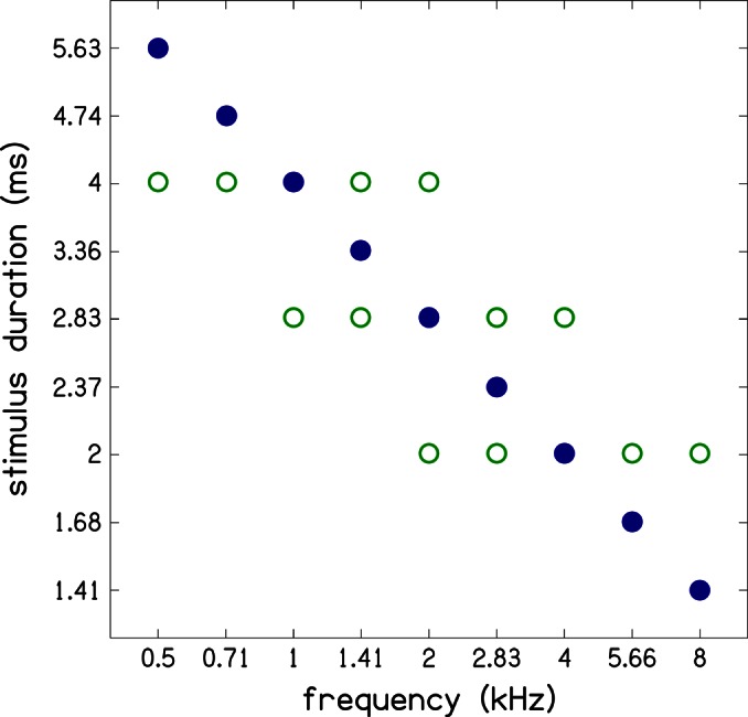
(Color online) Durations of tone-burst stimuli used at different frequencies. Four sets of stimulus durations were used in this study. In the first set (filled symbols), the duration (t_o) of the tone-bursts varied with frequency (f_o) according to $t_o\hspace{0.17em}=\hspace{0.17em}4/\sqrt{f_o}$ In the additional three sets (open symbols), the stimulus duration was held constant over a two-octave frequency range. Specifically, the constant stimulus duration of 4.00 ms was used for frequencies of 0.5–2 kHz, 2.83 ms was used for 1–4 kHz, and 2.00 ms for 2–8 kHz. Stimulus rise time is half the stimulus duration.

To improve the signal-to-noise ratio (SNR) of both ABR and TBOAE measurements and to improve the detectability of ABR wave V, more responses were included at low levels than at high levels. The stimulus was repeated 2048 times (1024 per buffer) for stimulus levels of 70–90 dB SPL, 4096 times at 50–60 dB SPL, and 8192 times for ≤40 dB SPL. Data were collected alternately into two buffers and separately for ABR and TBOAE measurement (i.e., a total of four buffers, two for TBOAE and two for ABR). The sum of the two buffers was used to provide an estimate of the signal. The difference between the two buffers used for the TBOAE measurement provided an estimate of the noise that was subsequently used as part of the data-acceptance criterion. TBOAE data were accepted if the SNR was 3 dB or greater. ABR data were accepted if a peak-to-trough wave V was observed for a range of stimulus levels. The acceptable criterion for ABR was monitored during data collection. The acceptable criterion for TBOAE was applied only after the data had been collected. There was no online monitoring of TBOAE responses for acoustic artifacts; however, whenever an ABR sweep was rejected during data collection because it did not meet the acceptable criterion for electrical artifacts, the corresponding TBOAE response was also rejected.

The combination of frequency, level, and duration resulted in a total of 168 stimulus conditions. Data collection typically required multiple sessions, each lasting about 2 h with some subjects returning for up to 21 h of data collection over several months. The 46 subjects included in this study did not contribute data at all test frequencies but contributed data based on their availability. Table TABLE I. shows the number of subjects who contributed data at each test frequency. A minimum of 11 subjects contributed data at 8 kHz and a maximum of 21 subjects contributed data at 4 kHz. In all, a total of 620 h of data-collection time were required to collect the data reported in this paper.

TABLE I.

Number of subjects contributing data at each test frequency.

Frequency (kHz)	Number of subjects
0.5	15
0.71	18
1	14
1.41	15
2	16
2.83	12
4	21
5.66	16
8	11

Analysis

ABR

Three individuals independently identified the ABR wave-V in the recorded waveform and scored its latency. The ABR wave-V latency was defined as the time between stimulus onset in the ear canal and the wave-V peak. We used this definition because this is what was used in our previous study (Gorga et al., 1988) and is in widespread use whenever ABR latencies are measured. Latencies were determined separately for averaged ABR waveforms (averaged over stimulus repetitions) from the two buffers used for data collection. The scorers used the high-level responses, which had a clearer wave-V peak, to help guide their identification of wave V in a level series of ABR responses, an approach which was particularly helpful for low-level conditions. Latencies were determined to a precision of 0.01 ms.

ABR forward latency τ_f (i.e., travel time1 of a particular frequency-component from stimulus onset to its characteristic cochlear place) was defined as

$${\tau }_f\hspace{0.17em}=\hspace{0.17em}{\tau }_{\text{wave}-\mathrm{V}}-\left({\tau }_{\text{synaptic}}+{\tau }_{\text{neural}}\right)\hspace{0.17em}\hspace{0.17em},$$ (2)

where τ_wave-V, τ_synaptic, and τ_neural are the measured wave-V latency, estimated synaptic delay (1 ms), and estimated neural-conduction delay (4 ms), respectively. τ_synaptic and τ_neural were assumed to be independent of frequency and level. τ_neural represents inter-peak delay between wave I and wave V. ABR forward latency was estimated separately for each of the four sets of stimulus durations.

Following Neely et al. (1988), we used the following equation to describe the dependence of total ABR latency on level and frequency

$${\widehat{\tau }}_{\text{wave}-\mathrm{V}}\hspace{0.17em}\hspace{0.17em}=\hspace{0.17em}\hspace{0.17em}a\hspace{0.17em}+\hspace{0.17em}b{c}^{-i}\hspace{0.17em}{f}^{-d}\hspace{0.17em}\hspace{0.17em},$$ (3)

where a is the sum (τ_synaptic + τ_neural), i is stimulus level divided by 100 dB SPL and f is stimulus frequency divided by 1 kHz. b, c, and d are constant parameters where c characterizes the level dependence, d characterizes the frequency dependence, and b is the latency that corresponds to a stimulus frequency of 1 kHz and a level of 0 dB SPL. From Eq. 3, ABR forward latency can be estimated by removing a = (τ_synaptic + τ_neural) = 5 ms, to obtain the power law

$$\widehat{\tau }{\hspace{0.17em}}_f\hspace{0.17em}\hspace{0.17em}=\hspace{0.17em}\hspace{0.17em}b{c}^{-1}\hspace{0.17em}\hspace{0.17em}{f}^{-d}.$$ (4)

This power-law fit to latency was also used by Harte et al. (2009) but without modeling for level dependence because they collected their data at only one level. The power-law fit was done in the log-log domain and the parameters b, c, and d were estimated by solving a multiple linear regression model using Gaussian elimination with partial pivoting. The description of the data using Eq. 4 allows for the evaluation and comparison of the level and frequency dependence of the latency for the different sets of stimulus durations used in this study and also allows for the comparison of the current latency data to data from previous studies.

OAE

The total acoustical response measured in the ear canal is a combination of the TBOAE, the stimulus, and noise. To estimate the TBOAE latency, a variation of the nonlinear residual method (Kemp et al., 1986) was used to extract the TBOAE from the total response. In the nonlinear residual method, a reference waveform is selected for each level series, at a given frequency, as the waveform that is judged to be at sufficiently high intensity that the TBOAE component is negligible compared to the stimulus component. In our variation of the nonlinear residual method, the reference signal was estimated from the highest level response using linear regression analysis. Let x_L(t) be a column vector with the response at the level of interest and x₉₀(t) be a column vector with the response at the highest level (which was 90 dB SPL in this case), then the linear regression model relating the two is

$$x{\hspace{0.17em}}_L\left(t\right)\hspace{0.17em}=\hspace{0.17em}\left[\mathrm{I} x_{90}\left(t\right)\right]\hspace{0.17em}\hspace{0.17em}X,$$ (5)

where I is a column of ones and X is the regression coefficients. Equation 5 expresses the response at the level of interest as linear combinations of the response at the reference level. The column of ones results in a matrix of coefficients with intercept parameters (or constant terms), which provides a better fit to the data. The coefficients X in Eq. 5 were calculated by Gaussian elimination with partial pivoting, and they include a constant term and a scale factor by which x₉₀(t) has to be scaled down to have the same level as x_L(t). Using the coefficients, an estimate of a reference signal that is appropriately scaled was obtained from the response at highest level as

$$\widehat{x}{\hspace{0.17em}}_L\left(t\right)={\left(\left[\mathrm{I} x_{90}\left(t\right)\right]X\right)}^T\hspace{0.17em}\hspace{0.17em},$$ (6)

where T denotes matrix transposition. An estimate of the TBOAE at the desired level y_L(t) was then obtain by subtraction as

$$y{\hspace{0.17em}}_L\left(t\right)=x_L\left(t\right)-{\widehat{x}}_L\left(t\right)\hspace{0.17em}\hspace{0.17em}.$$ (7)

Using linear regression to obtain the reference signal, as opposed to assuming a scale factor based on differences in stimulus levels between reference and desired responses, produces a scaling factor that takes into account effects that may result in improper scaling of the reference signal. For example, if the actual levels of x₉₀(t) and x_L(t) differed from the intended levels, scaling x₉₀(t) based on the intended level would result in incomplete cancellation of the stimulus. The constant term of the regression coefficients allows for compensation of non-zero mean or dc offset in the measured response, which further improves the estimation of the TBOAE. However, when this term is zero, our method is equivalent to the nonlinear residual method. Thus, the approach we have taken either provides estimates that are equivalent to those produced by the nonlinear residual method or produces a more accurate estimate of the residual. A limitation of our linear regression method is that it is only applicable in conditions where the stimulus and the OAE do not overlap much in time, such as TBOAE used here or click-evoked OAEs. The method would not be appropriate when the stimulus and OAE occur simultaneously as is the case for stimulus-frequency OAEs. After extracting the nonlinear residual, we zeroed the initial segment of the resultant waveform for a time equal to the duration of the stimulus plus 0.5 ms to further reduce residual stimulus artifact.

The latency of the TBOAE was calculated as the group delay in the time-domain (Rasetshwane and Neely, 2012; Shera and Bergevin, 2012) using

$${\tau }_{\mathit{O}\mathit{A}\mathit{E}}\hspace{0.17em}=\hspace{0.17em}\frac{{\displaystyle \sum _{t}t·{\left|y{\hspace{0.17em}}_L\left(t\right)\right|}^2}}{{\displaystyle \sum _t{\left|y{\hspace{0.17em}}_L\left(t\right)\right|}^2}},$$ (8)

This definition of group delay corresponds to the time at which the energy of y_L(t) is centered. The TBOAE y_L(t) was smoothed prior to the estimation of latency using a band pass filter centered at the tone-burst frequency and with a 1/3-octave passband. We elected to use energy-weighted group delay for TBOAE (which is different from the peak delay used for ABR) because it proved to be more reliable than delay based on TBOAE response peak. It was not always possible to pick out the peak corresponding to the TBOAE using automated procedures. Additionally, we could not translate energy-weighted group delay to peak delay because there are no universal procedures relating these two delay measures. The TBOAE latency estimates were also fitted with a power law of the form of Eq. 4 to model the dependence of latency on level and frequency. Fitting both ABR forward latency and TBOAE latency with the same power law allowed for comparison of the dependence of the two latencies on frequency and level.

RESULTS

Separate descriptions of ABR latency and TBOAE latency are presented first, followed by comparisons of ABR and TBOAE latencies.

ABR latency

Figure 2 shows average ABR wave-V latencies as a function of frequency for the four sets of stimulus durations. The parameter in each panel is stimulus level. For comparison, latency estimates for the frequency-dependent rise times (upper left panel) are superimposed as dashed lines in the plots for the latency estimates for constant durations. It was not always possible to determine the latency of wave V at the lowest level (20 dB SPL) because either the SNR was unfavorable or the wave-V peak was too broad, resulting in missing values for some conditions in Fig. 2. The ABR latencies for the frequency-dependent stimulus duration have an orderly frequency and level dependence. Latency is longer at low frequencies and decreases with increasing frequency. Latency is also longer at lower levels and decreases with increasing level. The latency estimates for the constant duration stimuli also show frequency and level dependence. However, the frequency dependence is not the same as that for the frequency-dependent stimulus duration, a point that will be discussed further with estimates of ABR forward latency.

Figure 2.

(Color online) ABR latencies as function of frequency for the four stimulus durations. Latencies for the stimulus duration $t_o\hspace{0.17em}=\hspace{0.17em}4/\sqrt{f_o}$ are superimposed as dashed lines in the other panels for comparison. There is an orderly dependence of latency on frequency and level for each stimulus condition. However, the frequency-dependence of the latency is stronger (steeper curve) for the stimulus duration data acquired using the frequency-dependent stimulus duration compared to the constant duration stimulus.

The variability of the ABR data was assessed using standard deviation (SD), and these SDs are presented in Table TABLE II. as function of frequency and level for the frequency-dependent stimulus duration. The SDs range from 0.0 to 1.6 ms with a grand mean SD of 0.6 ms. The mean SD is frequency dependent with lower SDs at higher frequencies. The mean SD is not systematically related to level but appears to be higher for mid-levels (60 dB SPL).

TABLE II.

Standard deviations of ABR latencies for frequency-dependent stimulus duration.

	0.5	0.71	1	1.41	2	2.83	4	5.66	8 kHz	Mean
20 dB SPL						0.01	0.55	0.61	0.63	0.45
30	0.22	0.02	0.46	0.82	0.58	0.66	0.61	0.57	0.48	0.49
40	0.91	0.74	0.69	0.88	0.88	0.54	0.51	0.52	0.49	0.68
50	1.39	0.97	0.86	0.91	0.57	0.53	0.45	0.45	0.39	0.72
60	1.64	1.44	1.30	0.76	0.46	0.45	0.42	0.38	0.38	0.80
70	1.17	1.25	1.16	0.68	0.43	0.43	0.34	0.34	0.31	0.68
80	0.65	0.92	0.73	0.41	0.46	0.42	0.28	0.31	0.32	0.50
90	0.69	0.62	0.53	0.42	0.37	0.34	0.24	0.23	0.30	0.42
mean	0.95	0.85	0.82	0.70	0.54	0.42	0.42	0.42	0.41	0.59

In Fig. 3, the present latency estimates for the set of frequency-dependent rise times are compared to previous latency estimates (Gorga et al., 1988) that used stimuli with similar (although not identical) rise times. The latencies are plotted in two panels with alternating levels to avoid clutter. Filled symbols represent the current data, and open symbols represent data from 1988. There is general agreement between the current measurement and the previous measurements except at 0.5 kHz where the current estimates are lower. The difference in latency at 0.5 kHz is probably due to differences in rise times of the tone-burst stimuli used in the two studies at this frequency. In the current study, a stimulus duration of 5.63 ms (rise time of 2.82 ms) was used while a stimulus duration of 12 ms (rise time of 4 ms) was used by Gorga et al. (1988); this results in longer latencies for the earlier study. Mean and standard deviation (SD) of the latency differences were used to quantify the similarities between the current ABR latencies and the earlier ABR latencies. The mean differences (across frequency and level) were 0.14 ms, and the mean SD of these differences was 0.41 ms. These mean ± SD values support the visual agreement observed in Fig. 3. The frequency dependence in the current latency estimates is also consistent with results of Harte et al. (2009), as discussed further in the following text.

Figure 3.

(Color online) Comparison of current ABR latency estimates forstimulus duration $t_o\hspace{0.17em}=\hspace{0.17em}4/\sqrt{f_o}$ to latency estimates of Gorga et al. (1988). There is agreement between the current latency estimates and the latency estimates from Gorga et al. (1988).

Figure 4 shows average ABR forward latencies (i.e., the presumed travel time of a particular frequency component from stimulus onset to its characteristic cochlear place) as a function of frequency with stimulus level as the parameter. Recall that ABR forward latency was estimated by subtracting estimates of synaptic and neural-conduction delays from the delay of wave V [cf. Eq. 2]. Data for different rise times are shown in each panel along with power-law fits to the data. Parameters b, c, and d of Eq. 4 are presented in the figure as inserts and in Table TABLE III.. Table TABLE III. also includes approximate uncertainties (95% confidence interval) for the parameters. All three parameters were statistically significant (p < 0.01) for all four stimulus rise-time conditions. The amount of variance accounted for by the fits (r²), is also presented in Fig. 4 and Table TABLE III.. The power-law fits provide good descriptors of the latency data for all four stimulus rise times, accounting for at least 96% of the variance. The value of parameter d, the exponent that characterizes the frequency dependence of latency, has an absolute value that is non-zero for all stimulus durations. This indicates that the latency varies with frequency in all cases. However, the value of d is larger in the case in which frequency-dependent stimulus rise times were used. This implies that the frequency dependence of the ABR latency is increased when the stimulus duration varies with frequency compared to when the stimulus duration is fixed. The values of parameter c are similar for the four rise-time conditions, indicating that there is similar level dependence for the different sets of stimulus durations.

Figure 4.

(Color online) ABR forward latency as a function of stimulus frequency. The symbols represent the same data presented in Fig. 2 but with 5 ms subtracted. The parallel lines are the power law fits to the data [see Eq. 4]. Parameters values for the power-law fit and R² values are included as inserts in the figure panels. Equation 4 accounts for at least 92% of the variance. There is frequency and level dependence for each set of stimulus durations. However, frequency dependence is stronger for the stimulus duration $t_o\hspace{0.17em}=\hspace{0.17em}4/\sqrt{f_o}$.

TABLE III.

Parameter values for power-law fits to the ABR forward latency data and amount of variance accounted for by the fits. Approximate uncertainties (i.e., 95% confidence interval) for the parameter values are also included. ABR forward latency varies more with frequency when the stimulus duration depends on frequency. The power-law fits account for at least 96% of the variance in the data.

Stimulus duration	b (ms)	c	d	R2 statistic
Frequency-dependent	12.63 ± 0.64	5.34 ± 0.41	0.39 ± 0.02	0.98
4.00 ms	13.89 ± 1.15	6.17 ± 0.78	0.22 ± 0.05	0.96
2.83 ms	11.47 ± 0.89	5.05 ± 0.57	0.31 ± 0.05	0.96
2.00 ms	9.99 ± 1.05	5.10 ± 0.58	0.24 ± 0.06	0.96

The present ABR forward latency estimates for the frequency-dependent duration can also be compared to the latency estimates described in Neely et al. (1988), using values obtained when fitting the data with Eq. 4. Neely et al. (1988) obtained parameter values of b = 12.9 ms, c = 5.0, and d = 0.41 in their fit to the latency data for frequency-dependent stimulus durations. We obtained values of b = 12.63 ± 0.64 ms, c = 5.34 ± 0.41, and d = 0.39 ± 0.02 for the present data set, which are similar to the earlier estimates. Comparison can also be made to parameters obtained by Harte et al. (2009), who also used stimulus durations that vary with frequency. Harte et al. (2009), obtained latency data with frequency dependence, d = 0.37, that is similar to the value that described our data. However, they did not model level dependence since their measurements were made at only one level.

TBOAE latency

Figure 5 shows average TBOAE latencies as a function of frequency with level as the parameter. Data for a different rise time are shown in each panel. Latency estimates for the frequency-dependent rise time are superimposed as dashed lines in the plots for the latency estimates for the three other rise times. Latency estimates for the frequency-dependent stimulus duration exhibit both level and frequency dependence, although the frequency dependence is not as strong or systematic as that of the ABR wave-V latency. Also, the latency at 4 kHz is shorter than the latency at higher frequencies for most levels. This effect cannot be due to standing waves, which have been shown to affect in-the-ear (ITE) stimulus calibration mostly near 4 kHz (e.g., Scheperle et al., 2008; Richmond et al., 2011) because ITE calibration was not used in this study. Even so, if the effect was due to a standing wave, it would also appear in the ABR latency (see Fig. 2), and not just the TBOAE latency, because the two were collected simultaneously. Despite the fact that we do not know why the TBOAE data at 4 kHz are outliers, we are able to rule out effects of standing waves because of our simultaneous data collection. This is a strength of the present paradigm, in which simultaneous collection of ABR and TBOAE data was used. The latency estimates at low levels (20–40 dB SPL) and low frequencies (0.5 and 0.71 kHz) show reduced level dependence. This is likely caused by the low SNR and a limitation of Eq. 8. Low SNR by itself makes the TBOAE measurements unreliable. In addition, the latency value obtained with Eq. 8 has an upper limit (16 ms + half the duration of the zeroed segment) at low SNRs because this equation calculates the location of the center of mass of the response. The latency at high frequencies (5.66 and 8 kHz) is overestimated due to the zeroing at the initial segment of the TBOAE response (necessary to reduce stimulus artifact), which includes response to high frequencies.

Figure 5.

(Color online) TBOAE latencies as function of frequency for the four stimulus durations. Latencies for the stimulus duration $t_o\hspace{0.17em}=\hspace{0.17em}4/\sqrt{f_o}$ are superimposed as dashed lines in the other panels for comparison. The latencies depend on level and frequency. However, the dependence is not as orderly compared to that of ABR latencies.

The latency estimates for the constant-duration stimuli also show level and frequency dependence, but the frequency dependence is reduced compared to the frequency-dependent duration case. The overestimation of latency at high frequencies (5.66 and 8 kHz) is greater for the constant duration of 2 ms compared to the case of the frequency-dependent duration. This is a result of the need for increased zeroing in the 2 ms duration case compared to the frequency- dependent duration case. Recall that the TBOAE response was zeroed for an interval that is equal to the stimulus duration plus 0.5 ms. The zeroed segments were the same (2.5 ms) at both 5.66 and 8 kHz for the constant-duration (2 ms) condition, but the zeroed segments differed (1.64 and 2.18 ms) at 5.66 and 8 kHz for the frequency-dependent condition. Thus it is more likely that some high-frequency responses were eliminated by the zeroing rule when the duration was fixed at 2 ms compared to when the stimulus duration depended on frequency.

The variability of the OAE data was also assessed using SDs, which are presented in Table TABLE IV. for all measured frequency and level conditions for the frequency-dependent rise-time condition. The SDs range from 1.0 to 5.0 ms, with a grand mean SD of 2.9 ms, and are approximately five times greater than the SDs for the ABR data. The mean SD does not show any systematic dependence on frequency. However, the mean SD depends on level, being larger at low levels. The smaller variability at high levels is due to favorable (larger) SNRs at higher levels, resulting in more reliable determinations of the group delay.

TABLE IV.

Standard deviations of TBOAE latencies for frequency-dependent stimulus duration. TBOAE latencies were five times more variable than ABR latencies.

	0.5	0.71	1	1.41	2	2.83	4	5.66	8 kHz	Mean
20 dB SPL	2.33	2.17	2.98	3.12	4.39	4.06	3.55	3.99	4.03	3.40
30	2.80	2.60	3.06	2.61	3.74	3.68	2.67	4.46	5.00	3.40
40	2.77	1.96	3.52	3.40	2.94	2.91	1.81	4.04	4.50	3.09
50	3.02	2.56	3.63	2.90	2.78	3.39	1.26	3.35	1.65	2.73
60	3.24	2.76	3.51	2.30	3.57	2.19	1.85	4.35	3.61	3.04
70	2.72	2.16	3.72	2.33	1.83	1.82	2.38	2.86	0.97	2.31
80	2.81	2.35	3.83	2.07	1.87	1.56	2.85	2.68	2.23	2.47
mean	2.81	2.37	3.46	2.68	3.02	2.80	2.34	3.68	3.14	2.92

In Fig. 6, the TBOAE latencies of Fig. 5 are re-plotted together with power-law fits to the latency in the log-log domain. Parameters b, c, and d of Eq. 4 are presented in the figure and in Table TABLE V.. Table TABLE V. also includes approximate uncertainties (95% confidence interval) for the parameters. Parameters b and c were statistically significant for all four stimulus durations (p < 0.01). However, parameter d, the exponent that characterizes the frequency dependence of latency was statistically significant only for two conditions: frequency-dependent stimulus duration and stimulus duration of 2.83 ms (p < 0.01). For the other two stimulus conditions, the value of parameter d was not statistically significant with p = 0.18 and p = 0.95 for stimulus durations of 4 and 2 ms, respectively. The amount of variability accounted for by the power-law fits (R²) is also presented in Fig. 6 and Table TABLE V.. The power-law fits account for 82% to 94% of the variance of the data. In the two cases where the value of parameter d was statistically significant, the frequency dependence of the TBOAE latency (d = 0.34 ± 0.06 and d = 0.37 ± 0.08 for frequency-dependent and 2.83 ms stimulus durations, respectively) was similar to that of the ABR forward latency (d = 0.39 ± 0.02 and d = 0.31 ± 0.05 for frequency-dependent and 2.83 ms stimulus durations, respectively). The value of d is close to zero for the other two durations (4.00 and 2.00 ms). These two cases include low and high frequencies, respectively. A value of d close to zero suggests that the latency does not depend on frequency. However, recall that latency estimates at low frequency are underestimated due to effects of low SNR and that latencies at high frequencies are overestimated due to effects on windowing of the TBOAE response. These constraints reduce accuracy of the power-law fits. The values of parameter c are similar to those obtained for ABR forward latency except for the case when the stimulus duration is 2.0 ms, which includes high frequencies. Again the overestimation of latency at high frequencies reduces accuracy of the power-law fits.

Figure 6.

(Color online) Power-law fits to TBOAE latency. When the data are reliable (frequency-dependent stimulus duration and stimulus duration = 2.83 ms), the frequency and level dependence of TBOAE latency is similar to that of ABR forward latency.

TABLE V.

Parameter values for power-law fits to the TBOAE latency data and amount of variance accounted for by the fits. Approximate uncertainties (i.e., 95% confidence interval) for the parameter values are included. When the TBOAE latency estimates are reliable (frequency-dependent stimulus duration and stimulus duration = 2.83 ms), their frequency and level dependence is similar to that of ABR forward latency. The power-law fits account for at least 82% of the variance in the data.

Stimulus duration	b (ms)	c	d	R2 statistic
Frequency-dependent	20.56 ± 2.85	6.44 ± 1.54	0.34 ± 0.06	0.84
4.00 ms	19.00 ± 1.44	4.75 ± 0.65	0.04 ± 0.06	0.94
2.83 ms	20.41 ± 2.27	6.06 ± 1.07	0.37 ± 0.08	0.93
2.00 ms	16.40 ± 4.16	9.32 ± 2.91	0.00 ± 0.15	0.82

Figure 7 compares our TBOAE latencies to TBOAE latencies of Harte et al. (2009) and to stimulus-frequency OAE (SFOAE) latencies of Shera and Guinan (2003). Specifically, the left panel compares our actual TBOAE latencies ±1 standard error (SE) obtained at a level of 60 dB SPL (triangles) and our power-law fit [cf. Eq. 4] to these data (dashed line) to a power-law function proposed by Harte et al.: τ = 10.98 f^−0.46 (solid line). Their data were collected at 66 dB peSPL. The two sets of TBOAE latencies have similar frequency dependence (similar slopes of power-law fits), but the latencies reported by Harte et al. are longer. The difference in the latencies might be due to differences in analyses methods or differences in calibration for stimulus level. In a similar manner, the right panel of Fig. 7 compares our TBOAE latencies ±1 SE at 40 dB SPL (circles) and power-law fit to these data (dashed line) to a power law function used by Shera and Guinan (2003) to model their data, which they collected at 40 dB SPL: τ = 11.0 f^−0.63 (solid line). The gray shading around the power-law function of Shera and Guinan describes the 95% confidence interval for their power-law fit. The SFOAE latencies are similar to our TBOAE latencies for frequencies between 0.71 and 4 kHz despite the fact that the frequency dependence of the two sets of data is different. Outside this range, the two latencies differ, with our TBOAE latencies being shorter at 0.5 kHz and longer for frequencies above 4 kHz. Possible reasons for these differences include the effects of SNR and zeroing of the initial TBOAE response, which were discussed earlier. However, it should be noted that the three sets of latencies are highly variable and as such these comparisons should be interpreted with caution.

Figure 7.

(Color online) Comparison of current TBOAE latencies to the TBOAE latencies of Harte et al. (2009) at 66 dB peSPL and to the SFOAE latencies of Shera and Guinan (2003) at 40 dB SPL. The shaded region describes the 95% confidence interval for the power-law fit reported by Shera and Guinan.

Relation between ABR forward latency and TBOAE latency

One of the objectives of this study was to determine the relationship between ABR forward latency and TBOAE latency by examining the ratio of TBOAE latency to ABR forward latency. To determine this relationship between these neural and mechanical estimates of peripherally determined latency, average TBOAE latencies were plotted against the corresponding average ABR forward latencies in a scatter plot. A simple linear regression model that describes the data was then determined using a fitting method that accounts for uncertainties in both latencies (Press et al., 1992). The slope of this regression line describes the ratio of TBOAE latency to ABR forward latency. This analysis was performed for three of the four stimulus durations, namely the frequency-dependent duration, constant duration of 4 ms and constant duration of 2 ms. Recall that frequency-dependent stimulus duration was used at all frequencies, while the 4 ms stimulus duration was used for low frequencies (0.5–2 kHz) and that the 2 ms stimulus duration was used for high frequencies (2–8 kHz). For the analysis based on frequency-dependent stimulus duration, separate simple linear regressions were fit to low and high frequencies. We wanted to analyze different frequency regions (low versus high) because previous studies have suggested that the dependence of OAE latency on frequency is different for high and low frequencies, that is, there is breakpoint in the latency-frequency relationship (e.g., Shera and Guinan 2003; Dhar et al., 2011; Rasetshwane and Neely, 2012).

Figure 8 includes scatter plots for the analysis comparing average ABR forward latencies to average TBOAE latencies along with simple linear regression lines fit to the data. From left to right, data are shown for durations of $t_o\hspace{0.17em}=\hspace{0.17em}4/\sqrt{f_o}$ (which includes all frequencies), t_o = 4 ms (with the analysis restricted to frequencies ≤ 1.5 kHz) and t_o = 2 ms (which only includes frequencies >1.5 kHz). The two different frequency regions are represented using closed symbols for low frequencies (≤1.5 kHz) and open symbols for high frequencies (>1.5 kHz), making it easier to compare separate frequency regions in the left panel of the figure. The four regression lines in Fig. 8 provide four estimates for the ratios of TBOAE latency to ABR forward latency, two for low frequencies and two for high frequencies. The goodness-of-fit for each regression line was acceptable, i.e., Q > 0.1 (see Press et al., 1992, p. 660 for definition of goodness-of-fit). The latency ratios (±95% confidence intervals) are r1_{f ≤ 1.5} = 1.33 ± 0.14 and r2_{f ≤ 1.5} = 1.37 ± 0.20 for low frequencies, and r1_f > 1.5 = 2.23 ± 0.16 and r2_f > 1.5 = 2.49 ± 0.15 for high frequencies. The two latency ratios for low frequency fits are similar, and the two latency ratios for the high frequency fits are similar. More importantly, comparison of latency ratios obtained for low frequency fits to those obtained for high frequency fits show statistically significant differences (confidence intervals for r1_{f ≤ 1.5} and r2_{f ≤ 1.5} do not overlap with confidence intervals for r1_f > 1.5 and r2_f > 1.5).

Figure 8.

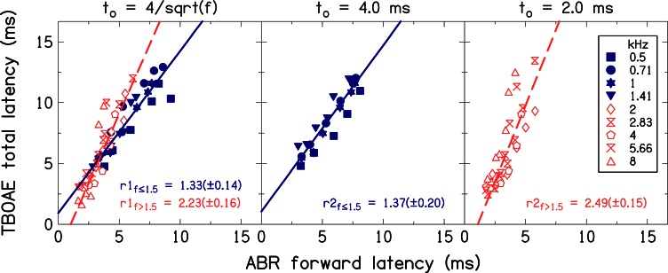
(Color online) Relationship between TBOAE latency and ABR forward latency. Filled symbols are used for low frequencies (≤1.5 kHz) and open symbols for high frequencies (>1.5 kHz). The solid and dashed lines are simple linear regression fits to the data at low and high frequencies, respectively. Slopes of the lines fit to the data are included as inserts in the figure panels. Uncertainties in the slope estimates (i.e., 95% confidence intervals) are also included. These slopes were used to represent the ratio of TBOAE latency to ABR forward latency.

The relationship between ABR latencies and TBOAE latencies was also investigated to determine the effect of rise time by analyzing the latencies as a function of level at a frequency where multiple rise times were used during data collection. Three stimulus rise times were used for the frequencies of 1.41, 2, and 2.83 kHz (see Fig. 1). We chose to evaluate the effects of rise time only at 2 kHz because the stimulus durations used at this frequency had the widest range, and if a rise-time effect was present, it would be evident at this frequency. Average latencies as function of level at 2 kHz are shown in Fig. 9 for ABRs (left panel) and TBOAEs (right panel). The parameter in each panel is duration. A two-way analysis of variance (ANOVA) was conducted to examine the effects of rise time (n = 3) and stimulus level (n = 7) on latency. Separate analyses were performed for ABR data at levels of 30–90 dB SPL (because there were few ABR data available at 20 dB SPL), and on TBOAE data at levels of 20 to 80 dB SPL, using the individual subject data. For ABR, there were significant effects of level F(6, 570) = 374.28, p < 0.05 and duration F(2, 570) = 3.46, p = 0.03. For TBOAE, there were also significant effects of level F(6, 570) = 37.52, p < 0.05 and duration F(2, 570) = 20.09, p < 0.05. The interaction between duration and level was not significant for either measurement; F(12, 570) = 0.76, p = 0.69 for ABR and F(12, 570) = 0.54, p = 0.89 for TBOAE. Thus, these results demonstrate that both ABR and TBOAE latencies depend on stimulus duration and level and that their dependence on one factor is independent of their dependence on the other factor.

Figure 9.

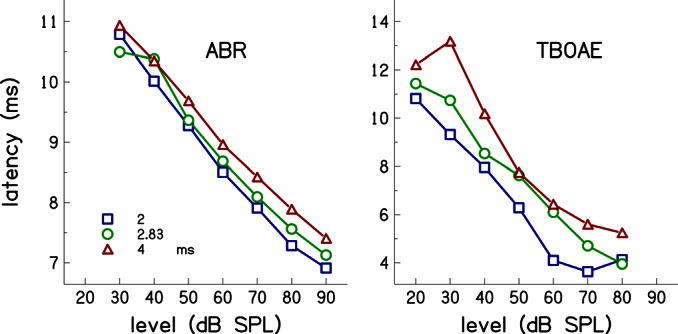
(Color online) ABR and TBOAE latencies at 2 kHz as function of stimulus level. The parameter is stimulus duration as indicated in the figure insert.

DISCUSSION

Simultaneous measurement of ABR and OAE latencies may provide insights into the effects of level, frequency, and stimulus rise time on cochlear delay. Comparison of these measurements may also provide information regarding issues such as (1) the physical generation mechanism of OAEs in the cochlea, (2) the place of reverse-wave generation, (3) the particular mode of reverse-wave propagation towards the base, and (4) the mechanism responsible for the level dependence of cochlear delay. We simultaneously measured ABR and TBOAE delays using a range of frequencies (0.5–8 kHz in 1/2-octave steps), levels (20–90 dB SPL in 10–dB steps), and rise times at each frequency. To our knowledge, simultaneous measurement of ABRs and TBOAEs has not previously been reported. Previous comparative studies made these measurements separately.

The ABR latencies had orderly frequency and level dependence with longer latencies at low frequencies and low levels. The measurements had small variability (grand mean SD of 0.59 ms) [cf. Table TABLE II. and were similar to the previous data reported by Gorga et al. (1988) (cf. Fig. 3). However, ABRs were not always measurable at 20 dB SPL for frequencies ≤2 kHz because the SNR was low, which made the identification of wave V difficult. This is the main reason for missing data in Fig. 2. Analysis of ABR forward latency (obtained by subtracting neural-conduction and synaptic delay) showed no interaction between its level dependence and its dependence on the rise time of the tone burst. However, the frequency dependence of the ABR latency was greater when the rise time of the tone burst varied with the frequency (cf. Fig. 4 and Table TABLE III.). The exponential variation of ABR latencies with increasing frequency, i.e., greater latency difference at low frequencies compared to high frequencies for a particular fixed stimulus level, is a characteristic feature of cochlear delay (see, e.g., Fig. 3 of Gorga et al., 1988; Fig. 7 of Tognola et al., 1997; Fig. 2 of Dhar et al., 2011). This feature is also present in our TBOAE latencies, although it is more difficult to observe because of the greater variability of these data. The exponential variation of cochlear latency is the reason why the frequency-latency relation appears as a straight line when plotted on log-log coordinates.

Several assumptions were made in the definition of ABR forward latency. First, we assumed that the latency of wave V is composed of a mechanical component that is due to the BM and a neural component due to the transmission along the auditory pathway above the level of the cochlea. Second, we assumed that the neural component (which includes neural conduction and synaptic delay) is relatively constant and does not depend significantly on frequency or level. The second assumption has been challenged by Ruggero and Temchin (2007), who assert that the neural contribution to ABR wave-V latency can be much longer than 5 ms. However, several studies support the current assumptions related to ABR latencies (e.g., Eggermont and Don, 1980; Don et al., 1993; Møller and Jannetta, 1983).

Ruggero and Temchin (2007) cite the first-spike latency measurements of Heil and Irvine (1997) in single auditory-nerve fibers as evidence that the level dependence of the onset of neural responses can exceed 30 ms. Indeed, Heil and Irvine report mean first-spike latencies in low-spontaneous-rate neurons (in response to tones with onset rise times of 1.7 ms) that decrease from 90 to 10 ms as the tone level increases from 30 to 50 dB SPL (see their Fig. 4B). However, first-spike latencies in single neurons are not the same as the latency of ABR Wave I, which is a compound action potential (CAP) that involves the synchronized response of many neurons. The change in first-spike latency observed by Heil and Irvine may have been influenced by non-evoked spikes due to spontaneous discharges. This interpretation is supported by the standard deviations of the first-spike latencies (see their Fig. 4D), which are about half of the mean values. Their observation interval was 200 ms, so randomly occurring (spontaneous) spikes would have a mean latency of 100 ms, which is close to the observed mean latency at the lowest level (30 dB SPL). Taken together, these two facts suggest that the apparent level dependence observed by Heil and Irvine in the first-spike latency was actually a transition from a low-level condition dominated by spontaneous discharges to a higher-level condition dominated by stimulus-evoked spikes. This mechanism of level dependence would not be observable in CAPs, which require synchronized discharges from many nerve fibers. Thus CAPs are always dominated by stimulus-evoked discharges. Additionally, the observed level dependence of the single-nerve-fiber, first-spike latency is much more abrupt in comparison to the consistent (∼1.6% per dB) level dependence that we observe in both ABR and TBOAE latency. In summary, the apparent difference in latency between the results reported here and those reported by Heil and Irvine (1997) may be the result of differences in the manner in which responses were measured and analyzed and not a reflection of disagreement in the fundamental findings.

The TBOAE latencies had level dependence that was similar to that of ABR latencies for all frequencies (cf. Fig. 5), although the TBOAE latencies were characterized by greater inter-subject variability by a factor of five [cf. Tables TABLE II. and TABLE IV.]. The accuracy of TBOAE-latency estimates may have been reduced by the presence of both stimulus artifacts (and/or the application of procedures to minimize the artifact) and acoustic noise. In the process of extracting the TBOAE response from the total recorded pressure waveform, we zeroed the initial segment of the waveform for a time equal to the duration of the stimulus plus 0.5 ms in efforts to remove the residual stimulus component that was not removed by the scale-and-subtract procedure. However, this zeroing removed some of the response to high-frequency stimuli (5.66 and 8 kHz), which have short latencies, potentially resulting in an overestimation of latency. The calculation of latency using Eq. 8 can also bias the latency when the SNR is low because at low SNRs, Eq. 8 has an upper limit that depends on the data-acquisition time (the limit is 16 ms + half the duration of the zeroed interval), as the equation calculates the center of mass of the response. To avoid this situation, an SNR criterion of 3 dB was applied. However, the SNR at 0.5 kHz was often low (slightly greater than 3 dB) resulting in underestimation of latency at this frequency. Similar issues with estimation of OAE latencies at low and high frequencies were discussed by Moleti and Sisto (2008). As a consequence of the difficulty of estimating TBOAE latencies at frequency extremes, the frequency dependence of TBOAE latencies can be reliably compared to that of ABR latency only for mid-frequencies in the current measurements. The difficulty in estimating OAE latencies is not unique to our study but has been encountered in other studies using techniques different from those used in the present study (e.g., Norton and Neely, 1987; Harte et al., 2009). Thus despite the fact that TBOAE latencies were estimated automatically and ABR latencies were estimated subjectively by three judges, there are lingering issues that complicate (and potentially contaminate) estimates of TBOAE latencies. As a consequence, we are cautious in our interpretation of these data.

The higher variability in the TBOAE latency measurements and uncertainties in the details of their analysis suggest that their interpretation and their comparison to ABR latencies should be made with some caution as pointed out by Moleti and Sisto (2008). We believe, however, that these problems were reduced by measuring the two latencies simultaneously; this provided comparable data on the same subject with the same stimuli and in the same laboratory.

Although the TBOAE latencies are always longer than the ABR latencies, the ratio of TBOAE latency to ABR forward latency depended on frequency (cf. Fig. 8). A higher ratio was observed for high frequencies (above 1.5 kHz) and a lower ratio was observed for low frequencies. We do not know why the ratios depend on frequency nor the implications of this observation. However, a delay ratio that is significantly greater than one but less than or equal to two might suggest that forward travel toward the characteristic place and reverse travel back to the cochlear base are both via a traveling wave. A ratio of two holds when the denominator of the ratio is a pressure delay like the TBOAE delay in the numerator, and a ratio less than two2 holds when the delay in the denominator is due to BM displacement (Shera et al., 2008). This contradicts the claims of Ren (2004) and others that OAEs travel backward by fast compression waves, especially considering that Ren's data are from the high-frequency region where we observed a ratio greater than two. A ratio close to one might suggests either (1) that there is a faster mode of reverse wave travel with shorter latency compared to the forward traveling wave or (2) that there are contributions to the outgoing signal from locations that are more basal than the locations that generate ABRs in response to the same frequencies. Nevertheless, the fact that the latency ratio at high frequencies is greater than 2 is not entirely consistent with the model of reverse traveling wave. Similarly, the fact that the ratio is greater than 1 at low frequencies is not entirely consistent with the model of fast compression wave for reverse propagation. On the other hand, it is important to point out that we may have obtained a latency ratio that is greater than two at high frequencies because our assumption that the neural-conduction and synaptic delays are always a constant 5 ms was not valid. If neural propagation time was shorter than assumed at high frequencies, then using a constant 5 ms would be too much for high-CF fibers. As a result, the forward ABR latency would be slightly underestimated at these frequencies and the delays ratios would appear to be greater than two. In summary, although there may have been some issues with our assumption regarding neural delay, we cannot use existing models to explain our data despite the fact that our experiment was designed to test compatibility with these models.

Results of an ANOVA showed that for both ABR and TBOAE latencies, there are significant effects of level and tone-burst rise time and that these effects are independent of each other (i.e., interaction was not significant). The fact that the dependence of ABR latency on tone-burst rise time is statistically independent of its level dependence suggests that the level dependence may be due to cochlear mechanics, which, in turn indicates that this level dependence is probably due to cochlear travel time.

CONCLUSION

ABR and TBOAE latencies have similar level dependence across frequencies. They also have similar frequency dependence at mid-frequencies where TBOAE latencies are most reliably measured. The level dependence of ABR latencies may include both mechanical and neural contributions, whereas TBOAE latencies are determined entirely by cochlear mechanics. The similarity at all frequencies of the level dependence of ABR latency to that of TBOAE latency supports the view that most of the level dependence of both measurements is due to cochlear mechanics. This view is further supported (1) by independence of level and rise-time effects and (2) by similarity of frequency dependence at mid-frequencies. Although TBOAE latency was always greater than ABR latency at the same frequency and level, the ratio of TBOAE to ABR latency was observed to depend on frequency, with a higher ratio at higher frequencies. This variable ratio does not support the use of existing models to completely explain our data.

References

- Burkard, R., and Secor, C. (2002). “ Overview of auditory evoked potential,” in Handbook of Clinical Audiology, edited by Katz J. (Lippincott, Williams, and Wilkins, Philadelphia, PA: ), Chap. 14, pp. 233–248. [Google Scholar]
- Dhar, S., Rogers, A., and Abdala, C. (2011). “ Breaking away: Violation of distortion emission phase-frequency invariance at low frequencies,” J. Acoust. Soc. Am. 129, 3115–3122. 10.1121/1.3569732 [DOI] [PMC free article] [PubMed] [Google Scholar]
- Don, M., Ponton, C. W., Eggermont, J. J., and Masuda, A. (1993). “ Gender differences in cochlear response time: An explanation for gender amplitude differences in the unmasked auditory brain stem response,” J. Acoust. Soc. Am. 94, 2135–2148. 10.1121/1.407485 [DOI] [PubMed] [Google Scholar]
- Dong, W., and Olson, E. S. (2008). “ Supporting evidence for reverse cochlear traveling waves,” J. Acoust. Soc. Am. 123, 222–240. 10.1121/1.2816566 [DOI] [PubMed] [Google Scholar]
- Eggermont, J. J., and Don, M. (1980). “ Analysis of the click-evoked brain stem potentials in humans using high-pass noise masking. II. Effect of click intensity,” J. Acoust. Soc. Am. 68, 1671–1675. 10.1121/1.385199 [DOI] [PubMed] [Google Scholar]
- Gorga, M. P. Kaminski, J. R., and Beauchaine, K. L. (1991). “ Effects of stimulus phase on the latency of the auditory brainstem response,” J. Am. Acad. Audiol. 2, 1–6. [PubMed] [Google Scholar]
- Gorga, M. P., Reiland, J. K., Beauchaine, K. A., and Jesteadt, W. (1988). “ Auditory brainstem responses to tone bursts in normal hearing subjects,” J. Speech Hear. Res. 31, 87–97. [DOI] [PubMed] [Google Scholar]
- Greenwood, D. D. (1990). “ A cochlear frequency-position function for several species—29 years later,” J. Acoust. Soc. Am. 87, 2592–2605. 10.1121/1.399052 [DOI] [PubMed] [Google Scholar]
- Harte, J. M., Pigasse, G., and Dau, T. (2009). “ Comparison of cochlear delay estimates using otoacoustic emissions and auditory brain stem responses,” J. Acoust. Soc. Am. 126, 1291–1301. 10.1121/1.3168508 [DOI] [PubMed] [Google Scholar]
- He, W., Nuttall, A. L., and Ren, T. (2007). “ Two-tone distortion at different longitudinal locations on the basilar membrane,” Hear. Res. 228, 112–122. 10.1016/j.heares.2007.01.026 [DOI] [PMC free article] [PubMed] [Google Scholar]
- Heil, P., and Irvine, D. R. (1997). “ First-spike timing of auditory-nerve fibers and comparison with auditory cortex,” J. Neurophysiol. 78, 2438–2454. [DOI] [PubMed] [Google Scholar]
- Kemp, D. T., Bray, P., Alexander, L., and Brown, A. M. (1986). “Acoustic emission cochleography–Practical aspects,” Scand. Audiol. Suppl. 25, 71–95. [PubMed] [Google Scholar]
- Kiang, N. Y. S., Watanabe, T., Thomas, E. C., and Clark L. F. (1965). Discharge Patterns of Single Fibers in the Cat's Auditory Nerve, MIT Research Monograph No. 35 (The MIT Press, Cambridge, MA: ), p. 154. [Google Scholar]
- Kim, D. O., and Molnar, C. E. (1979). “ A population study of cochlear nerve fibers: Comparison of spatial distributions of average-rate and phase-locking measures of responses to single tones,” J. Neurophysiol. 42, 16–30. [DOI] [PubMed] [Google Scholar]
- Moleti, A., and Sisto, R. (2008). “ Comparison between otoacoustic and auditory brain stem response latencies supports slow backward propagation of otoacoustic emissions,” J. Acoust. Soc. Am. 123, 1495–1503. 10.1121/1.2836781 [DOI] [PubMed] [Google Scholar]
- Møller, A. R., and Jannetta, P. J. (1983). “ Interpretation of brainstem auditory evoked-potentials: Results from intracranial recordings in humans,” Scand. Audiol. 12, 125–133. 10.3109/01050398309076235 [DOI] [PubMed] [Google Scholar]
- Neely, S. T., Norton, S., Gorga, M. P., and Jesteadt, W. (1988). “ Latency of auditory brain-stem responses and otoacoustic emissions using tone-burst stimuli,” J. Acoust. Soc. Am. 83, 652–656. 10.1121/1.396542 [DOI] [PubMed] [Google Scholar]
- Norton, S. J., and Neely, S. T. (1987). “ Tone-burst-evoked oto-acoustic emissions in normal hearing subjects,” J. Acoust. Soc. Am. 81, 1860–1872. 10.1121/1.394750 [DOI] [PubMed] [Google Scholar]
- Press, W. H., Teukolsky, S. A., Vetterling, W. T., and Flannery B. P. (1992) Numerical Recipes in C: The Art of Scientific Computing, 2nd ed. (Cambridge University Press, New York: ), pp. 656–670. [Google Scholar]
- Rasetshwane, D. M., and Neely, S. T. (2011). “ Inverse solution of ear-canal area function from reflectance,” J. Acoust. Soc. Am. 130, 3873–3881. 10.1121/1.3654019 [DOI] [PMC free article] [PubMed] [Google Scholar]
- Rasetshwane, D. M., and Neely, S. T. (2012). “ Measurements of wide-band cochlear reflectance in humans,” J. Assoc. Res. Otolaryngol. 13, 591–607. 10.1007/s10162-012-0336-1 [DOI] [PMC free article] [PubMed] [Google Scholar]
- Ren, T. (2004). “ Reverse propagation of sound in the gerbil cochlea,” Nat. Neurosci. 7, 333–334. 10.1038/nn1216 [DOI] [PubMed] [Google Scholar]
- Rhode, W. S. (1971). “Observations of the vibration of the basilar membrane in squirrel monkeys using the Mössbauer technique,” J. Acoust. Soc. Am. 49, 1218–1231. 10.1121/1.1912485 [DOI] [PubMed] [Google Scholar]
- Richmond, S. A., Kopun, J. G., Neely, S. T., Tan, H., and Gorga, M. P. (2011). “ Distribution of standing–wave errors in real-ear sound-level measurements,” J. Acoust. Soc. Am. 129, 3134–3140. 10.1121/1.3569726 [DOI] [PMC free article] [PubMed] [Google Scholar]
- Rønne, F. P., and Dau, T. (2012). “ Modeling auditory evoked brain stem responses to transient stimuli,” J. Acoust. Soc. Am. 131, 3903–3913. 10.1121/1.3699171 [DOI] [PubMed] [Google Scholar]
- Ruggero, M. A., and Temchin, A. N. (2007). “ Similarity of traveling-wave delays in the hearing organs of humans and other tetrapods,” J. Assoc. Res. Otolaryngol. 8, 153–166. 10.1007/s10162-007-0081-z [DOI] [PMC free article] [PubMed] [Google Scholar]
- Scheperle, R. A., Neely, S. T., Kopun, J. G., and Gorga, M. P. (2008). “ Influence of in situ sound level calibration on distortion product otoacoustic emission variability,” J. Acoust. Soc. Am. 124, 288–300. 10.1121/1.2931953 [DOI] [PMC free article] [PubMed] [Google Scholar]
- Schoonhoven, R., Prijs, V. F., and Schneider, S. (2001). “ DPOAE group delays versus electrophysiological measures of cochlear delay in normal human ears,” J. Acoust. Soc. Am. 109, 1503–1512. 10.1121/1.1354987 [DOI] [PubMed] [Google Scholar]
- Shera, C. A., and Bergevin, C. (2012). “ Obtaining reliable phase-gradient delays from otoacoustic emission data,” J. Acoust. Soc. Am. 132, 927–943. 10.1121/1.4730916 [DOI] [PMC free article] [PubMed] [Google Scholar]
- Shera, C. A., and Guinan, J. J., Jr. (2003). “ Stimulus-frequency emission group delay: A test of coherent reflection filtering and a window on cochlear tuning,” J. Acoust. Soc. Am. 113, 2762–2772. 10.1121/1.1557211 [DOI] [PubMed] [Google Scholar]
- Shera, C. A., Guinan, J. J., and Oxenham, A. J. (2010). “ Otoacoustic estimation of cochlear tuning: Validation in the chinchilla,” J. Assoc. Res. Otolaryngol. 11, 343–365. 10.1007/s10162-010-0217-4 [DOI] [PMC free article] [PubMed] [Google Scholar]
- Shera, C. A., Tubis, A., and Talmadge, C. L. (2005). “ Coherent reflection in a two-dimensional cochlea: Short-wave versus long-wave scattering in the generation of reflection-source otoacoustic emissions,” J. Acoust. Soc. Am. 118, 287–313. 10.1121/1.1895025 [DOI] [PubMed] [Google Scholar]
- Shera, C. A., Tubis, A., and Talmadge, C. L. (2008). “ Testing coherent reflection in chinchilla: Auditory-nerve responses predict stimulus-frequency emissions,” J. Acoust. Soc. Am. 124, 343–365. 10.1121/1.2917805 [DOI] [PMC free article] [PubMed] [Google Scholar]
- Shera, C. A., Tubis, A., Talmadge, C. L., de Boer, E., Fahey, P. F., and Guinan, J. J. (2007). “ Allen–Fahey and related experiments support the predominance of cochlear slow-wave otoacoustic emissions,” J. Acoust. Soc. Am. 121, 1564–1575. 10.1121/1.2405891 [DOI] [PubMed] [Google Scholar]
- Siegel, J. H., Cerka, A. J., Recio-Spinoso, A., Temchin, A. N., Van Dijk, P., and Ruggero, M. A. (2005). “ Delays of stimulus-frequency otoacoustic emissions and cochlear vibrations contradict the theory of coherent reflection filtering,” J. Acoust. Soc. Am. 118, 2434–2443. 10.1121/1.2005867 [DOI] [PubMed] [Google Scholar]
- Sisto, R., Moleti, A., Botti, T., Bertaccini, D., and Shera, C. A. (2011). “ Distortion products and backward-traveling waves in nonlinear active models of the cochlea,” J. Acoust. Soc. Am. 129, 3141–3152. 10.1121/1.3569700 [DOI] [PMC free article] [PubMed] [Google Scholar]
- Talmadge, C. L., Tubis, A., Long, G. R., and Piskorski, P. (1998). “ Modeling otoacoustic emission and hearing threshold fine structures,” J. Acoust. Soc. Am. 104, 1517–1543. 10.1121/1.424364 [DOI] [PubMed] [Google Scholar]
- Tognola, G., Ravazzani, P., and Grandori, F. (1997). “ Time-frequency distributions of click-evoked otoacoustic emissions,” Hear. Res. 106, 112–122. 10.1016/S0378-5955(97)00007-5 [DOI] [PubMed] [Google Scholar]
- Vetesnik, A., Nobili, R., and Gummer, A. (2006). “ How does the inner ear generate distortion product otoacoustic emissions? Results from a realistic model of the human cochlea,” ORL 68, 347–352. 10.1159/000095277 [DOI] [PubMed] [Google Scholar]
- Wilson, J. P. (1980). “ Model for cochlear echoes and tinnitus based on an observed electrical correlate,” Hear. Res. 2, 527–532. 10.1016/0378-5955(80)90090-8 [DOI] [PubMed] [Google Scholar]
- Wilson, M. (2008). “ Interferometry data challenge prevailing view of wave propagation in the cochlea,” Phys. Today 61, 26–27. [Google Scholar]
- Zweig, G., and Shera, C. A. (1995). “ The origin of periodicity in the spectrum of evoked otoacoustic emissions,” J. Acoust. Soc. Am. 98, 2018–2047. 10.1121/1.413320 [DOI] [PubMed] [Google Scholar]