Modeling the Spatial Spread of Rift Valley Fever in Egypt

Abstract

Rift Valley fever (RVF) is a severe viral zoonosis in Africa and the Middle East that harms both human health and livestock production. It is believed that RVF in Egypt has been repeatedly introduced by the importation of infected animals from Sudan. In this paper, we propose a three-patch model for the process by which animals enter Egypt from Sudan, are moved up the Nile, and then consumed at population centers. The basic reproduction number for each patch is introduced and then the threshold dynamics of the model are established. We simulate an interesting scenario showing a possible explanation of the observed phenomenon of the geographic spread of RVF in Egypt.

1 Introduction

Rift Valley fever (RVF) is a viral zoonosis of domestic animals (such as cattle, sheep, camels, and goats) and humans caused by the RVF virus (RVFV), a member of the genus Phlebovirus in the Bunyaviridae family. Initially identified in the Rift Valley of Kenya in 1931 (Daubney et al. 1931), outbreaks of RVF have been reported in sub-Saharan Africa, Egypt, Saudi Arabia, and Yemen (Abdo-Salem et al. 2011b). These result in significant economic losses due to high mortality and abortion in livestock. The virus is transmitted primarily by the bites of infected female mosquitoes. Several mosquito species of the genera Culex or Aedes are known vectors and some Aedes spp. can also transmit the virus vertically (mother-to-offspring). Humans can also become infected by direct/indirect contact with the blood or organs of infected animals, but they cannot transmit it (WHO 2010). To date, two types of vaccines are available for veterinary use (Ikegami and Makinob 2009), but there is no licensed vaccine for humans. Outbreaks of RVF in East Africa are typically associated with rainfall events (Linthicum et al. 1999; Anyamba et al. 2009). Heavy rainfall is believed to induce outbreaks by raising water levels in low-lying areas sufficiently to allow the hatching of Aedes spp. eggs, which can persist during dry periods. Since Aedes mosquitoes can transmit RVF vertically, the newly hatched mosquitoes can induce an outbreak once they mature (Favier et al. 2006). However, vertical transmission has not been demonstrated in some countries with substantial outbreaks of RVF. For example, the study of field-collected mosquitoes suggests that Culex pipiens is the main vector of RVFV in Egypt (Meegan et al. 1980). An alternative hypothesis is that in such regions outbreaks may occur when the disease is introduced by the importation of infected animals (Gad et al. 1986; Abdo-Salem et al. 2011a, 2011b) or by the use of live virus vaccines (Kamal 2011) together with suitable conditions for transmission, specifically high mosquito densities and the presence of large numbers of host animals (Abdo-Salem et al. 2011a, 2011b).

Mathematical models have become an important tool in identifying disease transmission processes, assessing infection risk and prevalence, and optimizing control strategies. However, so far little has been done to model and analyze the RVF transmission dynamics (Métras et al. 2011). Gaff et al. (2007) proposed a compartmental model to explore the mechanisms of RVFV circulation including Aedes and Culex mosquitoes and livestock population, in which each adult mosquito population is divided into classes containing susceptible, exposed and infectious individuals and the livestock population is classified as susceptible, exposed, infectious, and recovered. To account for vertical transmission in Aedes mosquitoes, compartments for uninfected and infected eggs are also included. Meanwhile, only uninfected eggs are included for Culex mosquitoes. They derived the basic reproduction number to assess the stability of the disease-free equilibrium and performed sensitivity analysis to determine the most significant model parameters for disease transmission. Mpheshe et al. (2011) modified the model in Gaff et al. (2007) to reduce egg classes of mosquitoes, include human population and exclude vertical transmission in mosquitoes. They gave conditions for the stability of the disease-free equilibrium and persistence of the disease. Sensitivity indices of the basic reproduction number and the endemic equilibrium were evaluated to study the relative importance of different factors responsible for RVF transmission and prevalence. It is believed that RVFV is introduced to a disease-free area by insects carried by wind and animal movements through trade (Métras et al. 2011). Xue et al. (2012) presented a network-based metapopulation model incorporating Aedes and Culex mosquitoes, livestock and human populations. They tested the model with data from an outbreak of RVF in South Africa and analyzed the sensitivity of the model to its parameters. Recently, Chamchod et al. (2012) proposed a simple but innovative model to investigate the emergence of RVF outbreaks, and epizootic and enzootic cycles of RVFV. Many aspects of their investigation have not been addressed in previous modeling studies. For example, they considered the effect of vaccination on the transmission dynamics of RVFV. However, these models either do not include spatial effects or are too complicated for rigorous mathematical analysis.

The main purpose of this paper is to propose a mathematically tractable model with spatial dynamics that can capture the hypothesis that Rift Valley fever outbreaks in Egypt might arise when the importation of large numbers of animals from Sudan coincides with high mosquito densities and there is an introduction of the infection during that period through importation of infected animals, use of live virus vaccines, or some other mechanism. In the next section, we develop a three-patch epidemic model to describe the spatial spread of RVF in Egypt. In Sect. 3, the basic reproduction number for each patch is calculated and the threshold dynamics of the model will be established. Moreover, the existence and stability of the endemic equilibrium are discussed. In Sect. 4, we simulate an interesting scenario showing possible explanation to the observed phenomenon of the geographic spread of RVF in Egypt. A brief discussion is given in Sect. 5.

2 The Model

The first outbreak of RVF in Egypt occurred in the Nile Valley and Delta in 1977 (Hoogstraal et al. 1979). This was the first RVF outbreak recorded outside traditionally affected areas in sub-Saharan Africa. Due to a combination of a lack of experience in dealing with RVF patients and insufficient public health programs, the outbreak caused at least thousands of human infections and hundreds of human deaths (Meegan 1979). Since then, Egypt has been experiencing continued RVF outbreaks among domestic animals, which indicates that the RVFV has become enzootic in Egypt. The imported animals from Sudan and the Horn of Africa were usually not vaccinated against RVFV. Travel time from north-central Sudan, where RVF was epizootic, to livestock markets in southern Egypt (Aswan Province), is less than 5 days, approximating the incubation period of RVFV in sheep (Gad et al. 1986; Abd el Rahim et al. 1999). So it is hypothesized that the recurrence of epizootics is mainly caused by the continuous importation of infected animals from Sudan and failure of the locally applied RVF vaccination program (Kamal 2011).

Egypt is an arid country with most of the population concentrated along the Nile, in the Delta and near the Suez Canal. The imported animals enter southern Egypt from northern Sudan, are moved up the Nile, and then consumed at population centers. At certain times, large numbers of animals are imported for holiday feasts. Vertical transmission of RVF has not been shown to occur in Egypt (Meegan et al. 1980). For simplicity, we restrict our focus to the disease transmission between domestic animals and mosquitoes, and ignore the age-dependent differential susceptibility and mortality in livestock. To capture the idea that more mosquitoes lead to more transmission, it seems most natural to use mass-action transmission terms. The movement timescale of animals is relatively short, so we assume that there is no host reproduction during the journey. Therefore, the density of hosts is determined by movement, mortality, and the rate at which they are introduced, which could be set to depend on demand. We assume that there is no movement for the vector population because of their limited mobility. We assume also that the mosquito population has logistic growth to maintain an equilibrium vector population. For epidemiology, we use a simple SIRS model for hosts and an SI model for vectors.

Based on the above assumptions, we propose a three-patch model (Sudan-Nile-feast) with animals movement from patch 1 to patch 2 and then from patch 2 to patch 3:

$$\{\begin{array}{c}\frac{d{S}_1}{dt}=r-{\alpha }_1{S}_1{V}_1-\mu S_1+\zeta R_1-\frac{c}{d_1}{S}_1,\hfill \\ \frac{d{I}_1}{dt}={\alpha }_1{S}_1{V}_1-(\mu +\gamma +\delta )I_1-\frac{c}{d_1}{I}_1,\hfill \\ \frac{d{R}_1}{dt}=\gamma I_1-(\mu +\zeta )R_1-\frac{c}{d_1}{R}_1,\hfill \\ \frac{d{U}_1}{dt}={\xi }_1(U_1+V_1)-\frac{{\xi }_1-{\nu }_1}{M_1}{(U_1+V_1)}^2-{\nu }_1{U}_1-{\beta }_1{I}_1{U}_1,\hfill \\ \frac{d{V}_1}{dt}={\nu }_1{V}_1+{\beta }_1{I}_1{U}_1,\hfill \end{array}\phantom{\}}$$ (1a)

$$\{\begin{array}{c}\frac{d{S}_2}{dt}=\frac{c}{d_1}{S}_1-{\alpha }_2{S}_2{V}_2-\mu S_2+\zeta R_2-\frac{c}{d_2}{S}_2,\hfill \\ \frac{d{I}_2}{dt}=\frac{c}{d_1}{I}_1+{\alpha }_2{S}_2{V}_2-(\mu +\gamma +\delta )I_2-\frac{c}{d_2}{I}_2,\hfill \\ \frac{d{R}_2}{dt}=\frac{c}{d_1}{R}_1+\gamma I_2-(\mu +\zeta )R_2-\frac{c}{d_2}{R}_2,\hfill \\ \frac{d{U}_2}{dt}={\xi }_2(U_2+V_2)-\frac{{\xi }_2-{\nu }_2}{M_2}{(U_2+V_2)}^2-{\nu }_2{U}_2-{\beta }_2{I}_2{U}_2,\hfill \\ \frac{d{V}_2}{dt}={\nu }_2{V}_2+{\beta }_2{I}_2{U}_2,\hfill \end{array}\phantom{\}}$$ (1b)

$$\{\begin{array}{c}\frac{d{S}_3}{dt}=\frac{c}{d_2}{S}_2-{\alpha }_3{S}_3{V}_3-\mu S_3+\zeta R_3-\frac{c}{d_3}{S}_3,\hfill \\ \frac{d{I}_3}{dt}=\frac{c}{d_2}{I}_2+{\alpha }_3{S}_3{V}_3-(\mu +\gamma +\delta )I_3-\frac{c}{d_3}{I}_3,\hfill \\ \frac{d{R}_3}{dt}=\frac{c}{d_2}{R}_2+\gamma I_3-(\mu +\zeta )R_3-\frac{c}{d_3}{R}_3,\hfill \\ \frac{d{U}_3}{dt}={\xi }_3(U_3+V_3)-\frac{{\xi }_3-{\nu }_3}{M_3}{(U_3+V_3)}^2-{\nu }_3{U}_3-{\beta }_3{I}_3{U}_3,\hfill \\ \frac{d{V}_3}{dt}=-{\nu }_3{V}_3+{\beta }_3{I}_3{U}_3.\hfill \end{array}\phantom{\}}$$ (1c)

The state variables and parameters used in model (1a)–(1c) and their descriptions are presented in Tables 1 and 2, respectively.

Table 1.

The state variables in model (1a)–(1c) and their descriptions

Symbol	Description
Si	Number of susceptible animals in patch i at time t
Ii	Number of infectious animals in patch i at time t
Ri	Number of recovered animals in patch i at time t
Ui	Number of susceptible mosquitoes in patch i at time t
Vi	Number of infectious mosquitoes in patch i at time t

Table 2.

The parameters in model (1a)–(1c) and their descriptions

Symbol	Description
r	Recruitment rate of animals
c	Movement speed of animals
di	The length of journey for animals within patch i
μ	Natural death rate for animals
δ	Disease-induced death rate for animals
γ	Recovery rate for animals
ζ	Rate of loss of immunity for animals
ξ i	Growth rate of mosquitoes in patch i
ν i	Natural death rate for mosquitoes in patch i
Mi	Carrying capacity for mosquitoes in patch i
α i	Transmission rate from vector to host in patch i
β i	Transmission rate from host to vector in patch i

The total number of mosquitoes in patch i at time t, denoted by $N_i^v\left(t\right)$, satisfies

$$\frac{d{N}_i^v}{dt}=({\xi }_i-{\nu }_i)N_i^v-\frac{{\xi }_i-{\nu }_i}{M_i}{\left(N_i^v\right)}^2,i=1,2,3,$$

and it converges to M_i as t → ∞ for any positive initial value. Let 1/p_i = d_i/c be the average time an animal spent in patch i. Therefore, we may consider the following reduced system:

$$\{\begin{array}{c}\frac{d{S}_1}{dt}=r-{\alpha }_1{S}_1{V}_1-\mu S_1+\zeta R_1-p_1{S}_1,\hfill \\ \frac{d{I}_1}{dt}={\alpha }_1{S}_1{V}_1-(\mu +\gamma +\delta )I_1-p_1{I}_1,\hfill \\ \frac{d{R}_1}{dt}=\gamma I_1-(\mu +\zeta )R_1-p_1{R}_1,\hfill \\ \frac{d{V}_1}{dt}=-{\nu }_1{V}_1+{\beta }_1{I}_1(M_1-V_1),\hfill \end{array}\phantom{\}}$$ (2a)

$$\{\begin{array}{c}\frac{d{S}_2}{dt}=p_1{S}_1-{\alpha }_2{S}_2{V}_2-\mu S_2+\zeta R_2-p_2{S}_2,\hfill \\ \frac{d{I}_2}{dt}=p_1{I}_1+{\alpha }_2{S}_2{V}_2-(\mu +\gamma +\delta )I_2-p_2{I}_2,\hfill \\ \frac{d{R}_2}{dt}=p_1{R}_1+\gamma I_2-(\mu +\zeta )R_2-p_2{R}_2,\hfill \\ \frac{d{V}_2}{dt}=-{\nu }_2{V}_2+{\beta }_2{I}_2(M_2-V_2),\hfill \end{array}\phantom{\}}$$ (2b)

$$\{\begin{array}{c}\frac{d{S}_3}{dt}=p_2{S}_2-{\alpha }_3{S}_3{V}_3-\mu S_3+\zeta R_3-p_3{S}_3,\hfill \\ \frac{d{I}_3}{dt}=p_2{I}_2+{\alpha }_3{S}_3{V}_3-(\mu +\gamma +\delta )I_3-p_3{I}_3,\hfill \\ \frac{d{R}_3}{dt}=p_2{R}_2+\gamma I_3-(\mu +\zeta )R_3-p_3{R}_3,\hfill \\ \frac{d{V}_3}{dt}=-{\nu }_3{V}_3+{\beta }_3{I}_3(M_3-V_3),\hfill \end{array}\phantom{\}}$$ (2c)

Theorem 2.1 All forward solutions in ${\mathbb{R}}_{+}^{12}$ of (2a)–(2c) eventually enter Ω = Ω₁ × Ω₂ × Ω₃, where ${\Omega }_i=\left\{\right(S_i,I_i,R_i,V_i)\in {\mathbb{R}}_{+}^4:S_i+I_i+R_i\le r{\prod }_{j=1}^i\frac{p_{j-1}}{\mu +p_j},V_i\le M_i$, i = 1, 2, 3, and p₀ = 1, and Ω is positively invariant for (2a)–(2c).

Proof Let $N_i^h\left(t\right)$ be the total host population in patch i at time t. Then we have

$$\frac{d{N}_1^h}{dt}=r-(\mu +p_1)N_1^h-\delta I_1\le r-(\mu +p_1)N_1^h$$

and

$$\frac{d{N}_i^h}{dt}=p_{i-1}{N}_{i-1}^h-(\mu +p_i)N_i^h-\delta I_i\le p_{i-1}{N}_{i-1}^h-(\mu +p_i)N_i^h,i=2,3.$$

By a simple comparison theorem (Smith and Waltman 1995), the proof is complete.

3 Mathematical Analysis

It is easy to see that (2a)–(2c) has a unique disease-free equilibrium

$$\begin{array}{cc}\hfill E^0& =(S_1^0,I_1^0,R_1^0,V_1^0,S_2^0,I_2^0,R_2^0,V_2^0,S_3^0,I_3^0,R_3^0,V_3^0)\hfill \\ \hfill & =\left(\frac{r}{\mu +p_1},0,0,0,\frac{r{p}_1}{(\mu +p_1)(\mu +p_2)},0,0,0,\frac{r{p}_1{p}_2}{(\mu +p_1)(\mu +p_2)(\mu +p_3)},0,0,0\right).\hfill \end{array}$$

Note that system (2a)–(2c) is in a block-triangular form, the dynamics of patch 1 are independent of patch 2 and patch 3 while the dynamics of patch 2 are independent of patch 3.

3.1 The First Patch

Obviously, $E_1^0=(S_1^0,0,0,0)$ is the unique disease-free equilibrium of subsystem (2a). To calculate the basic reproduction number corresponding to (2a), we order the infected state variables by (I₁, R₁, V₁). Following the method and notations of van den Driessche and Watmough (2002), the linearization of (2a) at $E_1^0$ gives

$$F=\left[\begin{array}{ccc}\hfill 0\hfill & \hfill 0\hfill & \hfill {\alpha }_1{S}_1^0\hfill \\ \hfill 0\hfill & \hfill 0\hfill & \hfill 0\hfill \\ \hfill {\beta }_1{M}_1\hfill & \hfill 0\hfill & \hfill 0\hfill \end{array}\right]\text{and}V=\left[\begin{array}{ccc}\hfill \mu +\gamma +\delta +p_1\hfill & \hfill 0\hfill & \hfill 0\hfill \\ \hfill -\gamma \hfill & \hfill \mu +\zeta +p_1\hfill & \hfill 0\hfill \\ \hfill 0\hfill & \hfill 0\hfill & \hfill {\nu }_1\hfill \end{array}\right].$$

Direct calculation yields

$$V^{-1}=\left[\begin{array}{ccc}\hfill {(\mu +\gamma +\delta +p_1)}^{-1}\hfill & \hfill 0\hfill & \hfill 0\hfill \\ \hfill \gamma {(\mu +\gamma +\delta +p_1)}^{-1}{(\mu +\zeta +p_1)}^{-1}\hfill & \hfill {(\mu +\zeta +p_1)}^{-1}\hfill & \hfill 0\hfill \\ \hfill 0\hfill & \hfill 0\hfill & \hfill {\nu }_1^{-1}\hfill \end{array}\right]$$

and the basic reproduction number for the first patch equals

$${\mathcal{R}}_{10}=\rho \left(F{V}^{-1}\right)=\sqrt{\frac{{\alpha }_1{S}_1^0}{{\nu }_1}\cdot \frac{{\beta }_1{M}_1}{\mu +\gamma +\delta +p_1}}=\sqrt{\frac{{\alpha }_{1}r}{(\mu +p_1){\nu }_1}\cdot \frac{{\beta }_1{M}_1}{\mu +\gamma +\delta +p_1}},$$

which depends on all parameters except ζ, the rate of loss of immunity for animals. ${\left({\mathcal{R}}_{10}\right)}^2$ is proportional to $S_1^0$ and M₁, so more mosquitoes and more animals lead to more disease transmission.

Theorem 3.1 The disease-free equilibrium $E_1^0$ of (2a) is globally asymptotically stable in Ω₁ if ${\mathcal{R}}_{10}\le 1$ and unstable if ${\mathcal{R}}_{10}>1$.

Proof It is easy to show the local stability or instability of $E_1^0$ by verifying (A1)–(A5) in van den Driessche and Watmough (2002).

Consider a Lyapunov function L₁ = ν₁(μ + p₁)I₁ + α₁rV₁ on Ω₁. Then

$$\begin{array}{cc}\hfill L_1^{\prime }& ={\nu }_1(\mu +p_1)I_1^{\prime }+{\alpha }_{1}r{V}_1^{\prime }\hfill \\ \hfill & ={\nu }_1(\mu +p_1){\alpha }_1{S}_1{V}_1-{\nu }_1(\mu +p_1)(\mu +\gamma +\delta +p_1)I_1-{\alpha }_{1}r{\nu }_1{V}_1+{\alpha }_{1}r{\beta }_1{I}_1(M_1-V_1)\hfill \\ \hfill & =\left[{\nu }_1\right(\mu +p_1){\alpha }_1{S}_1-{\alpha }_{1}r{\nu }_1]V_1+\left[{\alpha }_{1}r{\beta }_1\right(M_1-V_1)-{\nu }_1(\mu +p_1\left)\right(\mu +\gamma +\delta +p_1\left)\right]I_1\hfill \\ \hfill & ={\nu }_1(\mu +p_1){\alpha }_1(S_1-S_1^0)V_1+\left[{\alpha }_{1}r{\beta }_1\right(M_1-V_1)-{\nu }_1(\mu +p_1\left)\right(\mu +\gamma +\delta +p_1\left)\right]I_1\hfill \\ \hfill & \le =\left[{\alpha }_{1}r{\beta }_1\right(M_1-V_1)-{\nu }_1(\mu +p_1\left)\right(\mu +\gamma +\delta +p_1\left)\right]I_1\text{in}{\Omega }_1\hfill \\ \hfill & \le [{\alpha }_{1}r{\beta }_1-{\nu }_1(\mu +p_1\left)\right(\mu +\gamma +\delta +p_1\left)\right]I_1\hfill \\ \hfill & =\left[\right({\mathcal{R}}_{10}^2-1\left){\nu }_1\right(\mu +p_1\left)\right(\mu +\gamma +\delta +p_1\left)\right]I_1\hfill \\ \hfill & \le 0\text{if}{\mathcal{R}}_{10}\le 1.\hfill \end{array}$$

The largest compact invariant set, denoted by Γ₁, in $\left\{\right(S_1,I_1,R_1,V_1)\in {\Omega }_1:L_1^{\prime }=0\}$ is the singleton $\left\{E_1^0\right\}$.

Case 1: ${\mathcal{R}}_{10}<1$ The preceding calculation shows that I₁ ≡ 0. So,

$$\frac{d{V}_1}{dt}=-{\nu }_1{V}_1\text{and}\frac{d{R}_1}{dt}=-(\mu +\zeta +p_1)R_1.$$

Backward continuation of a compact invariant set indicates that V₁ = 0 and R₁ = 0. Thus,

$$\frac{d{S}_1}{dt}=r-(\mu +p_1)S_1.$$

This means that $S_1=S_1^0$ and hence ${\Gamma }_1=\left\{E_1^0\right\}$.

Case 2: ${\mathcal{R}}_{10}=1$ The preceding calculation gives either V₁ ≡ 0 or I₁ ≡ 0. The latter case proceeds as before. Suppose V₁ ≡ 0, then $\frac{d{V}_1}{dt}={\beta }_1{I}_1{M}_1\equiv 0$ which implies I₁ = 0. Once again this can proceed as before.

By LaSalle's invariance principle (LaSalle 1976), $E_1^0$ is globally asymptotically stable in Ω₁.

Theorem 3.2 If ${\mathcal{R}}_{10}>1$, then system (2a) has a unique endemic equilibrium, de noted by $E_1^{\ast }=(S_1^{\ast },I_1^{\ast },R_1^{\ast },V_1^{\ast })$, which is locally asymptotically stable. Moreover, the disease is uniformly persistent in ${\Omega }_1^0$, the interior of Ω₁, i.e., there is a constant ∊ > 0 such that any solution of (2a) starting at a point of ${\Omega }_1^0$ satisfies

$$\underset{t\to \infty }{\text{lim}\text{inf}}\left(I_1\left(t\right),R_1\left(t\right),V_1\left(t\right)\right)>(∊,∊,∊).$$

Proof If $E_1^{\ast }=(S_1^{\ast },I_1^{\ast },R_1^{\ast },V_1^{\ast })$ is a positive equilibrium of (2a), then it satisfies the following system of algebraic equations:

$$\begin{array}{cc}\hfill & r-{\alpha }_1{S}_1{V}_1-\mu S_1+\zeta R_1-p_1{S}_1=0,\hfill \\ \hfill & {\alpha }_1{S}_1{V}_1-(\mu +\gamma +\delta )I_1-p_1{I}_1=0,\hfill \\ \hfill & \gamma I_1-(\mu +\zeta )R_1-p_1{R}_1=0,\hfill \\ \hfill & -{\nu }_1{V}_1+{\beta }_1{I}_1(M_1-V_1)=0.\hfill \end{array}$$ (3)

Solving for S₁, R₁, and V₁ in terms of I₁ from the last three equations of (3), that is,

$$S_1=\frac{(\mu +\gamma +\delta +p_1)({\nu }_1+{\beta }_1{I}_1)}{{\alpha }_1{\beta }_1{M}_1},R_1=\frac{\gamma I_1}{\mu +\zeta +p_1},V_1=\frac{{\beta }_1{I}_1{M}_1}{{\nu }_1+{\beta }_1{I}_1},$$

and substituting them into the first equation, we obtain

$$r-(\mu +\gamma +\delta +p_1)I_1-(\mu +p_1)\frac{\mu +\gamma +\delta +p_1}{{\alpha }_1{\beta }_1{M}_1}({\beta }_1{I}_1+{\nu }_1)+\zeta \frac{\gamma }{\mu +\zeta +p_1}{I}_1=0,$$

which can be simplified to a linear equation

$$\left[(\mu +\gamma +\delta +p_1)+(\mu +p_1)\frac{\mu +\gamma +\delta +p_1}{{\alpha }_1{M}_1}-\frac{\zeta \gamma }{\mu +\zeta +p_1}\right]I_1+\left[(\mu +p_1)\frac{\mu +\gamma +\delta +p_1}{{\alpha }_1{\beta }_1{M}_1}{\nu }_1-r\right]=0.$$

The coefficient of I₁ is always positive and the constant part is negative if and only if ${\mathcal{R}}_{10}>1$. Hence, system (2a) has a unique endemic equilibrium if and only if ${\mathcal{R}}_{10}>1$.

Next we study the local stability of $E_1^{\ast }$ by using the Routh–Hurwitz criterion. The Jacobian matrix of system (2a) at the endemic equilibrium $E_1^{\ast }$ is

$$J(S_1^{\ast },I_1^{\ast },R_1^{\ast },V_1^{\ast })=\left(\begin{array}{cccc}\hfill -{\alpha }_1{V}_1^{\ast }-\rho \hfill & \hfill 0\hfill & \hfill \zeta \hfill & \hfill -{\alpha }_1{S}_1^{\ast }\hfill \\ \hfill {\alpha }_1{V}_1^{\ast }\hfill & \hfill -(\rho +\gamma +\delta )\hfill & \hfill 0\hfill & \hfill {\alpha }_1{S}_1^{\ast }\hfill \\ \hfill 0\hfill & \hfill \gamma \hfill & \hfill -(\rho +\zeta )\hfill & \hfill 0\hfill \\ \hfill 0\hfill & \hfill {\beta }_1(M_1-V_1^{\ast })\hfill & \hfill 0\hfill & \hfill -{\nu }_1-{\beta }_1{I}_1^{\ast }\hfill \end{array}\right),$$

where ρ = μ + p₁ and the corresponding characteristic equation is

$$P_1\left(\lambda \right)=(\lambda +\rho +\zeta )({\lambda }^3+b_2{\lambda }^3+b_1\lambda +b_0)-\zeta {\alpha }_1{V}_1^{\ast }\gamma (\lambda +{\nu }_1+{\beta }_1{I}_1^{\ast })=0,$$

where

$$\begin{array}{cc}\hfill b_2& ={\alpha }_1{V}_1^{\ast }+2\rho +\gamma +\delta +{\nu }_1+{\beta }_1{I}_1^{\ast }>0,\hfill \\ \hfill b_1& =({\alpha }_1{V}_1^{\ast }+\rho )(\rho +\gamma +\delta )+({\alpha }_1{V}_1^{\ast }+2\rho +\gamma +\delta )({\nu }_1+{\beta }_1{I}_1^{\ast })-{\alpha }_1{\beta }_1{S}_1^{\ast }(M_1-V_1^{\ast }),\hfill \\ \hfill b_0& =({\alpha }_1{V}_1^{\ast }+\rho )(\rho +\gamma +\delta )({\nu }_1+{\beta }_1{I}_1^{\ast })-{\alpha }_1{\beta }_1{S}_1^{\ast }\rho (M_1-V_1^{\ast }).\hfill \end{array}$$

It follows from the second and fourth equations of (3) that

$$(\rho +\gamma +\delta ){\nu }_1={\alpha }_1{\beta }_1{S}_1^{\ast }(M_1-V_1^{\ast })$$

and hence

$$\begin{array}{cc}\hfill b_1& =({\alpha }_1{V}_1^{\ast }+\rho )(\rho +\gamma +\delta +{\nu }_1)+({\alpha }_1{V}_1^{\ast }+2\rho +\gamma +\delta ){\beta }_1{I}_1^{\ast }>0,\hfill \\ \hfill b_0& =(\rho +\gamma +\delta )({\alpha }_1{\nu }_1{V}_1^{\ast }+{\alpha }_1{\beta }_1{V}_1^{\ast }{I}_1^{\ast }+\rho {\beta }_1{I}_1^{\ast })>0\text{and}{b}_1{b}_2>b_0.\hfill \end{array}$$

Then

$$P_1\left(\lambda \right)={\lambda }^4+c_3{\lambda }^3+c_2{\lambda }^2+c_1\lambda +c_0=0,$$

where

$$\begin{array}{cc}\hfill c_3& =\rho +\zeta +b_2>0,c_2=(\rho +\zeta )b_2+b_1>0,\hfill \\ \hfill c_1& =(\rho +\zeta )b_1+b_0-\zeta {\alpha }_1{V}_1^{\ast }\gamma =\rho b_1+b_0+\zeta (b_1-{\alpha }_1{V}_1^{\ast }\gamma )>0,\hfill \\ \hfill c_0& =(\rho +\zeta )b_0-\zeta {\alpha }_1{V}_1^{\ast }\gamma ({\nu }_1+{\beta }_1{I}_1^{\ast })=\rho b_0+\zeta (b_0-{\alpha }_1{V}_1^{\ast }\gamma ({\nu }_1+{\beta }_1{I}_1^{\ast }\left)\right)>0.\hfill \end{array}$$

Now it suffices to show that $c_1{c}_2{c}_3>c_1^2+c_3^2{c}_0$. In fact,

$$\begin{array}{cc}\hfill c_1& c_2{c}_3-c_1^2-c_3^2{c}_0\hfill \\ \hfill & =c_1(c_2{c}_3-c_1)-c_3^2{c}_0\hfill \\ \hfill & =c_1\left[c_3\right(\rho +\zeta )b_2+(b_1{b}_2-b_0)+\zeta {\alpha }_1{V}_1^{\ast }\gamma ]-c_3^2{c}_0\hfill \\ \hfill & >c_1{c}_3(\rho +\zeta )b_2-c_3^2{c}_0=c_3\left[c_1\right(\rho +\zeta )b_2-c_3{c}_0]\hfill \\ \hfill & =c_3\left[{(\rho +\zeta )}^2\right(b_1{b}_2-b_0)-\zeta {\alpha }_1{V}_1^{\ast }\gamma ((\rho +\zeta )b_2-(\rho +\zeta +b_2)({\nu }_1+{\beta }_1{I}_1^{\ast })\left)\right]\hfill \\ \hfill & >c_3\left[\right(\rho +\zeta \left)\zeta \right(b_1{b}_2-b_0)-\zeta {\alpha }_1{V}_1^{\ast }\gamma (\rho +\zeta \left)b_2\right]\hfill \\ \hfill & =c_3(\rho +\zeta )\zeta (b_1{b}_2-b_0-{\alpha }_1{V}_1^{\ast }\gamma b_2)>0.\hfill \end{array}$$

Thus, the Routh–Hurwitz criterion implies that all eigenvalues of the characteristic equation have negative real parts. Hence, the endemic equilibrium is locally asymptotically stable.

Finally, the uniform persistence of system (2a) in ${\Omega }_1^0$ can be proved by applying Theorem 4.6 in Thieme (1993). We omit the proof here, since it is similar to that of Theorem 2.5 in Gao and Ruan (2011).

Remark 3.3 It is worth mentioning that Yang et al. (2010) studied a similar vector-host epidemic model with an SIR structure for the host population and without disease-induced host deaths. They used the method of the second additive compound matrix (see Li and Muldowney 1996 and references therein) to establish the global stability of the endemic equilibrium when it exists. Unfortunately, we cannot use that approach to establish the global result because of the higher complexity in our model.

3.2 The Second Patch

By a simple comparison theorem, we conclude that the disease is uniformly persistent in Ω⁰ if it is uniformly persistent in ${\Omega }_1^0$. Namely, the disease will persist in all three patches if ${\mathcal{R}}_{10}>1$. Indeed, it follows from Theorem 3.2 that for any fixed initial data we have

$$\frac{d{I}_2}{dt}\ge p_1∊-(\mu +\gamma +\delta +p_2)I_2$$

for t large enough. So, lim inf_t→∞I₂(t) ≥ p₁∊/(μ + γ + δ + p2). Similarly, we can find positive lower limits for all other variables. If the disease dies out in patch 1, i.e., ${\mathcal{R}}_{10}\le 1$, then each solution of (2a) with nonnegative initial data converges to $E_1^0$ and the limiting system of (2b) is

$$\begin{array}{cc}\hfill \frac{d{S}_2}{dt}& =p_1{S}_1^0-{\alpha }_2{S}_2{V}_2-\mu S_2+\zeta R_2-p_2{S}_2,\hfill \\ \hfill \frac{d{I}_2}{dt}& ={\alpha }_2{S}_2{V}_2-(\mu +\gamma +\delta )I_2-p_2{I}_2,\hfill \\ \hfill \frac{d{R}_2}{dt}& =\gamma I_2-(\mu +\zeta )R_2-p_2{R}_2,\hfill \\ \hfill \frac{d{V}_2}{dt}& ={\nu }_2{V}_2+{\beta }_2{I}_2(M_2-V_2).\hfill \end{array}$$ (4)

Comparing (4) with (2a), we immediately find that (4) possesses a unique disease-free equilibrium $E_2^0=(S_2^0,I_2^0,R_2^0,V_2^0)=(p_1{S}_1^0∕(\mu +p_2),0,0,0)=(r{p}_1∕((\mu +p_1)(\mu +p_2)),0,0,0)$ and obtain the basic reproduction number of patch 2 as

$${\mathcal{R}}_{20}=\sqrt{\frac{{\alpha }_2{S}_2^0}{{\nu }_2}\cdot \frac{{\beta }_2{M}_2}{\mu +\gamma +\delta +p_2}}=\sqrt{\frac{{\alpha }_{2}r{p}_1}{(\mu +p_1)(\mu +p_2){\nu }_2}\cdot \frac{{\beta }_2{M}_2}{\mu +\gamma +\delta +p_2}}.$$

If ${\mathcal{R}}_{10}\le 1$ and ${\mathcal{R}}_{20}\le 1$, then the disease goes extinct in the first two patches; if ${\mathcal{R}}_{10}\le 1$ and ${\mathcal{R}}_{20}>1$, then the disease dies out in the first patch but persists in the last two patches.

3.3 The Third Patch

Similarly, if ${\mathcal{R}}_{10}\le 1$ and ${\mathcal{R}}_{20}\le 1$, we obtain a limiting system of (2c) as follows:

$$\begin{array}{cc}\hfill \frac{d{S}_3}{dt}& =p_2{S}_2^0-{\alpha }_3{S}_3{V}_3-\mu S_3+\zeta R_3-p_3{S}_3,\hfill \\ \hfill \frac{d{I}_3}{dt}& ={\alpha }_3{S}_3{V}_3-(\mu +\gamma +\delta )I_3-p_3{I}_3,\hfill \\ \hfill \frac{d{R}_3}{dt}& =\gamma I_3-(\mu +\zeta )R_3-p_3{R}_3,\hfill \\ \hfill \frac{d{V}_3}{dt}& =-{\nu }_3{V}_3+{\beta }_3{I}_3{U}_3.\hfill \end{array}$$ (5)

System (5) has a unique disease-free equilibrium $E_3^0=(S_3^0,I_3^0,R_3^0,V_3^0)=(p_2{S}_2^0∕(\mu +p_3),0,0,0)=(r{p}_1{p}_2∕((\mu +p_1)(\mu +p_2)(\mu +p_3)),0,0,0)$ and the basic reproduction number of patch 3 is given by

$$\begin{array}{cc}\hfill {\mathcal{R}}_{30}& =\sqrt{\frac{{\alpha }_3{S}_3^0}{{\nu }_3}\cdot \frac{{\beta }_3{M}_3}{\mu +\gamma +\delta +p_3}}\hfill \\ \hfill & =\sqrt{\frac{{\alpha }_{3}r{p}_1{p}_2}{(\mu +p_1)(\mu +p_2)(\mu +p_3){\nu }_3}\cdot \frac{{\beta }_3{M}_3}{\mu +\gamma +\delta +p_3}}.\hfill \end{array}$$

If ${\mathcal{R}}_{10}\le 1$, ${\mathcal{R}}_{20}\le 1$, and ${\mathcal{R}}_{30}\le 1$, then the disease goes extinct in all three patches; if ${\mathcal{R}}_{10}\le 1$, ${\mathcal{R}}_{20}\le 1$, and ${\mathcal{R}}_{30}>1$, then the disease dies out in the first two patches, but persists in the third patch. So, we have the following result.

Theorem 3.4 For the full model (2a)–(2c), if ${\mathcal{R}}_{10}>1$, the disease persists in all three patches; if ${\mathcal{R}}_{10}\le 1$ and ${\mathcal{R}}_{20}>1$, the disease dies out in the first patch but persists in the remaining two patches; if ${\mathcal{R}}_{10}\le 1$, ${\mathcal{R}}_{20}\le 1$, and ${\mathcal{R}}_{30}>1$, the disease dies out in the first two patches, but persists in the last patch; if ${\mathcal{R}}_{10}\le 1$, ${\mathcal{R}}_{20}\le 1$, and ${\mathcal{R}}_{30}\le 1$, the disease dies out in all three patches and E⁰ is globally asymptotically stable

Theorem 3.5 System (2a)–(2c) has a unique endemic equilibrium, denoted $E^{\ast }=(S_1^{\ast },I_1^{\ast },R_1^{\ast },V_1^{\ast },S_2^{\ast },I_2^{\ast },R_2^{\ast },V_2^{\ast },S_3^{\ast },I_3^{\ast },R_3^{\ast },V_3^{\ast })$, if and only if ${\mathcal{R}}_{10}>1$ and it is locally asymptotically stable when it exists.

Proof The necessity is a straightforward consequence of Theorem 3.1. To prove the existence and uniqueness of an endemic equilibrium as ${\mathcal{R}}_{10}>1$, it suffices to show that the system

$$\begin{array}{cc}\hfill \frac{d{S}_i}{dt}& =p_{i-1}{S}_{i-1}^{\ast }-{\alpha }_i{S}_i{V}_i-\mu S_i+\zeta R_i-p_i{S}_i,\hfill \\ \hfill \frac{d{I}_i}{dt}& =p_{i-1}{I}_{i-1}^{\ast }+{\alpha }_i{S}_i{V}_i-(\mu +\gamma +\delta )I_i-p_i{I}_i,\hfill \\ \hfill \frac{d{R}_i}{dt}& =p_{i-1}{R}_{i-1}^{\ast }+\gamma I_i-(\mu +\zeta )R_i-p_i{R}_i,\hfill \\ \hfill \frac{d{V}_i}{dt}& =-{\nu }_i{V}_i+{\beta }_i{I}_i(M_i-V_i),\hfill \end{array}$$ (6)

has a unique positive equilibrium for i = 2, 3. To compute the constant solution of (6), we set the right-hand side of each of the four equations equal to zero and direct calculations yield

$$p_{i-1}{S}_{i-1}^{\ast }+p_{i-1}{I}_{i-1}^{\ast }-(\mu +\gamma +\delta +p_i)I_i-(\mu +p_i)\frac{(\mu +\gamma +\delta +p_i)I_i-p_{i-1}{I}_{i-1}^{\ast }}{{\alpha }_i}\cdot \frac{{\beta }_i{I}_i+{\nu }_i}{{\beta }_i{M}_i{I}_i}+\zeta \frac{p_{i-1}{R}_{i-1}^{\ast }+\gamma I_i}{\mu +\zeta +p_i}=0,$$

which can be reduced to a quadratic equation

$$f\left(I_i\right)\equiv a_2{I}_i^2+a_1{I}_i+a_0=0,$$ (7)

where $a_2=-(1+\frac{\mu +p_i}{{\alpha }_i{M}_i})(\mu +\gamma +\delta +p_i)+\zeta \frac{\gamma }{\mu +\zeta +p_i}<0$, $a_1=p_{i-1}{S}_{i-1}^{\ast }+p_{i-1}{I}_{i-1}^{\ast }-\frac{\mu +p_i}{{\alpha }_i{\beta }_i{M}_i}\left(\right(\mu +\gamma +\delta +p_i){\nu }_i-p_{i-1}{I}_{i-1}^{\ast }{\beta }_i)+\zeta \frac{p_{i-1}{R}_{i-1}^{\ast }}{\mu +\zeta +p_i}$ and $a_0=\frac{\mu +p_i}{{\alpha }_i{\beta }_i{M}_i}{p}_{i-1}{I}_{i-1}^{\ast }{\nu }_i>0$.

Thus, (7) has exactly one positive root, $I_i^{\ast }$. To check the positivity of other variables, we need to verify that $I_i^{\ast }>p_{i-1}{I}_{i-1}^{\ast }∕(\mu +\gamma +\delta +p_i)$, or equivalently, $f(p_{i-1}{I}_{i-1}^{\ast }∕(\mu +\gamma +\delta +p_i\left)\right)>0$. In fact, $f(p_{i-1}{I}_{i-1}^{\ast }∕(\mu +\gamma +\delta +p_i\left)\right)$ equals

$$\frac{\zeta \gamma p_{i-1}^2{\left(I_{i-1}^{\ast }\right)}^2}{(\mu +\zeta +p_i){(\mu +\gamma +\delta +p_i)}^2}+\frac{p_{i-1}^2{S}_{i-1}^{\ast }{I}_{i-1}^{\ast }}{\mu +\gamma +\delta +p_i}+\frac{\zeta p_{i-1}^2{R}_{i-1}^{\ast }{I}_{i-1}^{\ast }}{(\mu +\zeta +p_i)(\mu +\gamma +\delta +p_i)}>0.$$

The local stability of the endemic equilibrium ($S_i^{\ast }$, $I_i^{\ast }$, $R_i^{\ast }$, $V_i^{\ast }$) of system (6) can be proved in a way similar to that of $E_1^{\ast }$ in Theorem 3.2.

3.4 Model with Permanent Immunity

Research in RVF indicates that an infection leads to a durable, probably life-long, immunity in animals (Paweska et al. 2005). In any event, the immunity period is relatively longer than the duration of movement. We may assume that the rate of loss of immunity ζ equals zero and use an SIR model for the host population. In this case, since R_i does not appear in other equations of (2a)–(2c), system (2a)–(2c) can be reduced to

$$\{\begin{array}{c}\frac{d{S}_1}{dt}=r-{\alpha }_1{S}_1{V}_1-\mu S_1-p_1{S}_1,\hfill \\ \frac{d{I}_1}{dt}={\alpha }_1{S}_1{V}_1-(\mu +\gamma +\delta )I_1-p_1{I}_1,\hfill \\ \frac{d{V}_1}{dt}=-{\nu }_1{V}_1+{\beta }_1{I}_1(M_1-V_1),\hfill \end{array}\phantom{\}}$$ (8a)

$$\{\begin{array}{c}\frac{d{S}_2}{dt}=p_1{S}_1-{\alpha }_2{S}_2{V}_2-\mu S_2-p_2{S}_2,\hfill \\ \frac{d{I}_2}{dt}=p_1{I}_1+{\alpha }_2{S}_2{V}_2-(\mu +\gamma +\delta )I_2-p_2{I}_2,\hfill \\ \frac{d{V}_2}{dt}=-{\nu }_2{V}_2+{\beta }_2{I}_2(M_2-V_2),\hfill \end{array}\phantom{\}}$$ (8b)

$$\{\begin{array}{c}\frac{d{S}_3}{dt}=p_2{S}_2-{\alpha }_3{S}_3{V}_3-\mu S_3-p_3{S}_3,\hfill \\ \frac{d{I}_3}{dt}=p_2{I}_2+{\alpha }_3{S}_3{V}_3-(\mu +\gamma +\delta )I_3-p_3{I}_3,\hfill \\ \frac{d{V}_3}{dt}=-{\nu }_3{V}_3+{\beta }_3{I}_3(M_3-V_3).\hfill \end{array}\phantom{\}}$$ (8c)

The following result can be proved in a way similar to that of Theorem 4.3 in Yang et al. (2010). Consequently, the disease dynamics of (8a)–(8c) are completely determined by the basic reproduction numbers ${\mathcal{R}}_{i0}$ for i = 1, 2, 3.

Theorem 3.6 For system (8a)–(8c), if ${\mathcal{R}}_{10}>1$, then the disease persists at an endemic equilibrium level in all three patches; if ${\mathcal{R}}_{10}\le 1$ and ${\mathcal{R}}_{20}>1$, then the disease dies out in the first patch but persists at an endemic equilibrium level in the remaining two patches; if ${\mathcal{R}}_{10}\le 1$, ${\mathcal{R}}_{20}\le 1$, and ${\mathcal{R}}_{30}\le 1$, then the disease dies out in the first two patches, but persists at an endemic equilibrium level in the last patch; if ${\mathcal{R}}_{10}\le 1$, ${\mathcal{R}}_{20}\le 1$, and ${\mathcal{R}}_{30}\le 1$, then the disease dies out in all three patches.

3.5 The Relation Between ${\mathcal{R}}_{i0}$ and Model Parameters

It follows from Theorem 3.4 that the disease dies out in all patches if and only if ${\mathcal{R}}_{i0}\le 1$ for i = 1, 2, 3. In other words, to eliminate the disease from the whole system, all three threshold parameters ${\mathcal{R}}_{10}$, ${\mathcal{R}}_{20}$, and ${\mathcal{R}}_{30}$ must be reduced to be less than 1. To do so, we should study how the basic reproduction numbers vary with the model parameters, which can help us design highly efficient control strategies. Recall that

$${\mathcal{R}}_{i0}^2=\frac{{\alpha }_{i}r}{{\nu }_i}\prod _{j=1}^i\frac{p_{j-1}}{\mu +p_j}\cdot \frac{{\beta }_i{M}_i}{\mu +\gamma +\delta +p_i},p_i=\frac{c}{d_i},i=1,2,3,\text{and}{p}_0=1.$$

Obviously, ${\mathcal{R}}_{i0}$ is strictly increasing in α_i, β_i, M_i, r, or d_i, and strictly decreasing in ν_i, μ, γ, δ, or d_j, j = 1, …, i − 1. An increase in the movement speed, c, will decrease ${\mathcal{R}}_{i0}$. The dependence of ${\mathcal{R}}_{i0}$ on c, becomes more complicated if i > 1, since c appears in both the numerator and denominator of the formula for ${\mathcal{R}}_{i0}^2$.

Proposition 3.7 For i > 1, there exists some $c_i^{\ast }$ such that the basic reproduction number ${\mathcal{R}}_{i0}$ is strictly increasing in c if c ∈ (0, $c_i^{\ast }$) and strictly decreasing if c ∈ ($c_i^{\ast }$, ∞). Furthermore, $(i-1)\mu {\underset{¯}{d}}_i∕2<c_i^{\ast }<(i-1)\mu {\stackrel{‒}{d}}_i$, where d_i = min_1≤j≤i d_j and ${\stackrel{‒}{d}}_i={\max }_{1\le j\le i}{d}_j$.

Proof Let g_i(c) be the partial derivative of ${\mathcal{R}}_{i0}$ with respect to c. Then

$$\begin{array}{cc}\hfill g_i\left(c\right)& =\frac{{\alpha }_{i}r{\beta }_i{M}_i}{{\nu }_i}\cdot \frac{\partial }{\partial c}\left(\prod _{j=1}^i\frac{p_{j-1}}{\mu +p_j}\cdot \frac{1}{\mu +\gamma +\delta +p_i}\right)\hfill \\ \hfill & =\frac{{\alpha }_{i}r{\beta }_i{M}_i}{{\nu }_i}\cdot \frac{\partial }{\partial c}\left(\prod _{j=1}^i\frac{1}{\mu d_j+c}\cdot \frac{c^{i-1}{d}_i^2}{(\mu +\gamma +\delta )+d_i+c}\right)\hfill \\ \hfill & =\frac{{\alpha }_{i}r{\beta }_i{M}_i}{{\nu }_i}\cdot c^{i-2}{d}_i^2\cdot \frac{(i-1)D\left(c\right)-c\cdot D^{\prime }\left(c\right)}{D^2\left(c\right)}\hfill \\ \hfill & =\frac{{\alpha }_{i}r{\beta }_i{M}_i}{{\nu }_i}\cdot c^{i-2}{d}_i^2\cdot \left((i-1)D\left(c\right)-c\left(\sum _{j=1}^i\frac{D\left(c\right)}{\mu d_j+c}+\frac{D\left(c\right)}{(\mu +\gamma +\delta )d_i+c}\right)\right)∕D^2\left(c\right)\hfill \\ \hfill & =\frac{{\alpha }_{i}r{\beta }_i{M}_i}{{\nu }_i}\cdot c^{i-2}{d}_i^2\cdot \left((i-1)-c\left(\sum _{j=1}^i\frac{1}{\mu d_j+c}+\frac{1}{(\mu +\gamma +\delta )d_i+c}\right)\right)∕D\left(c\right),\hfill \end{array}$$

where $D_i\left(c\right)=\left(\right(\mu +\gamma +\delta )d_i+c){\prod }_{j=1}^i(\mu d_j+c)$ and the sign of g_i(c) is the same as that of

$$h_i\left(c\right)=(i-1)-c\left(\sum _{j=1}^i\frac{1}{\mu d_j+c}+\frac{1}{(\mu +\gamma +\delta )d_i+c}\right).$$

Since h_i (0) = (i − 1) > 0, h(∞) = −2 and h′ (c) < 0 for c ≥ 0, the equation h_i(c) = 0 has exactly one positive root, denoted by $c_i^{\ast }$, satisfying h_i(c) > 0 if c ∈ (0, $c_i^{\ast }$) and h_i(c) < 0 if c ∈ ($c_i^{\ast }$, ∞). Note that

$$h_i\left(k\mu d\right)=(i-1)-\sum _{j=1}^i\frac{kd}{d_j+kd}-\frac{k\mu d}{(\mu +\gamma +\delta )d_i+k\mu d}\text{for}k>0\text{and}d>0.$$

In particular, we have

$$\begin{array}{cc}\hfill & h_i\left(\right(i-1\left)\mu {\stackrel{‒}{d}}_i\right)\le (i-1)-i\cdot \frac{i-1}{1+(i-1)}-\frac{(i-1)\mu {\stackrel{‒}{d}}_i}{(\mu +\gamma +\delta )d_i+(i-1)\mu {\stackrel{‒}{d}}_i}<0,\hfill \\ \hfill & h_i\left(\right(i-1)\mu {\underset{¯}{d}}_i∕2)>(i-1)-i\cdot \frac{i-1}{i+1}-\frac{i-1}{i+1}=0,i>1,\hfill \end{array}$$

which implies $c_i^{\ast }\in \left(\right(i-1)\mu {\underset{¯}{d}}_i∕2,(i-1\left)\mu {\stackrel{‒}{d}}_i\right)$.

Remark 3.8 The duration of movement in each patch, 1/p_i = d_i/c, is about a few weeks or months, while the life span of an animal, 1/μ, could be a couple of years or even longer. Namely, the timescale of the movement is very short relative to the host population dynamic timescale. So generally speaking, ${\mathcal{R}}_{i0}$ is decreasing in c and shortening the duration of host movement could reduce the possibility of a disease spread.

Now we perform a sensitivity analysis of the basic reproduction number ${\mathcal{R}}_{i0}$ to model parameters to determine how best to reduce initial disease transmission. The normalized forward sensitivity index (Chitnis et al. 2008) or elasticity of ${\mathcal{R}}_{i0}$ to a parameter p is defined as

$${{\rm Y}}_p^i=\frac{\partial {\mathcal{R}}_{i0}}{{\partial }_p}\times \frac{p}{{\mathcal{R}}_{i0}}.$$

For i = 1, 2, 3, we find that ${{\rm Y}}_{{\alpha }_i}^i={{\rm Y}}_{{\beta }_i}^i={{\rm Y}}_{M_i}^i={{\rm Y}}_r^i=\frac{1}{2}$, ${{\rm Y}}_{{\nu }_i}^i=-\frac{1}{2}$, ${{\rm Y}}_{\gamma }^i=-\frac{\gamma }{2(\mu +\gamma +\delta +p_i)}>-\frac{1}{2}$ and ${{\rm Y}}_{\delta }^i=-\frac{\delta }{2(\mu +\gamma +\delta +p_i)}>-\frac{1}{2}$. In addition, if $c\gg \mu {\stackrel{‒}{d}}_i$ then

$$\begin{array}{cc}\hfill {{\rm Y}}_{\mu }^i& =-\frac{1}{2}\left(\sum _{j=1}^i\frac{\mu d_j}{\mu d_j+c}+\frac{\mu d_i}{(\mu +\gamma +\delta )d_i+c}\right)>-\frac{1}{2},\hfill \\ \hfill {{\rm Y}}_{d_j}^i& =-\frac{1}{2}\frac{\mu d_j}{(\mu d_j+c)}>-\frac{1}{2},\text{for}j=1,\dots ,i-1,\hfill \\ \hfill {{\rm Y}}_{d_i}^i& =\frac{1}{2}c\left(\frac{1}{\mu d_j+c}+\frac{1}{(\mu +\gamma +\delta )d_i+c}\right)>\frac{1}{2},\text{and}{{\rm Y}}_c^i=\frac{1}{2}{h}_i\left(c\right)<-\frac{1}{2}.\hfill \end{array}$$

It follows from ${{\rm Y}}_{d_i}^i>-{{\rm Y}}_c^i$ that ${\mathcal{R}}_{i0}$ is most sensitive to the travel distance in the ith patch, d_i. However, the travel route is usually fixed, and thus the most feasible way for fast reducing ${\mathcal{R}}_{i0}$ is to accelerate livestock transport.

4 Numerical Simulations

In this section, we conduct numerical simulations to confirm our analytical results. The model uses a daily time step and some of the parameter values are chosen from the data in Gaff et al. (2007) and the references therein.

Firstly, we explore the relation between ${\mathcal{R}}_{i0}$ and the travel speed c. We use the following set of parameter values: r = 300, μ = 1.2 × 10⁻³, δ 0.1, γ 0.4, ζ = 5 × 10⁻³, M₁ = 1000, M₂ = 8000, M₃ = 1500, d₁ = 100, d₂ = 800, d₃ = 200, ν_i = 0.06, α_i = 3 × 10⁻⁵ and β_i = 8 × 10⁻⁵ for i 1, 2, 3. Figure 1 shows how the basic reproduction number varies as a function of the livestock movement rate c, in the range c ∈ [0, 40]. As predicted by Proposition 3.7, the curve of ${\mathcal{R}}_{10}$ is constantly decreasing, and the curves of ${\mathcal{R}}_{20}$ and ${\mathcal{R}}_{30}$ are increasing for small c and then decreasing.

Fig. 1.

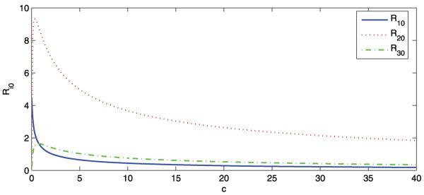
The curves of the basic reproduction number of patch i, ${\mathcal{R}}_{i0}$, versus c

Now we fix c at 25 and the respective basic reproduction numbers are ${\mathcal{R}}_{10}=0.2522<1$, ${\mathcal{R}}_{20}=2.352>1$, and ${\mathcal{R}}_{30}=0.4672<1$. To consider a hypothetical disease invasion scenario, we set the initial data of patches 2 and 3 to zero such that there are no infected animals or mosquitoes in patches 2 and 3 at the beginning of travel. The disease dies out in patch 1, but persists in patches 2 and 3, which is consistent with Theorem 3.4 (see Figs. 2 and 3). This may represent an interesting phenomenon regarding the role that animal movement plays in the spatial spread of RVF from Sudan to Egypt. Though the disease is introduced to patch 2 from patch 1, it goes extinct in its origin because of lower mosquito density in patch 1. Patch 2 (the Nile) has high mosquito population density and the disease will reach an endemic level once it appears. Patch 3 cannot sustain a disease alone, but this becomes possible because of continuous immigration of infected animals from patch 2.

Fig. 2.

Numerical simulations of system (2a) showing I_i vs. t. Initial conditions: S₁(0) = 1800, I₁(0) = 50, R₁(0) = 100, V₁(0) = 0, and S₂(0) = I₂(0) = R₂(0) = V₂(0) = S₃(0) = I₃(0) = R₃(0) = V₃(0) = 0. ${\mathcal{R}}_{10}<1$, ${\mathcal{R}}_{20}>1$, and ${\mathcal{R}}_{30}>1$

Fig. 3.

Numerical simulations of system (2a) showing V_i vs. t. Initial conditions: S₁(0) = 1800, I₁(0) = 50, R₁(0) = 100, V₁(0) = 0, and S₂(0) = I₂(0) = R₂(0) = V₂(0) = S₃(0) = I₃(0) = R₃(0) = V₃(0) = 0. ${\mathcal{R}}_{10}<1$, ${\mathcal{R}}_{20}>1$, and ${\mathcal{R}}_{30}>1$

5 Discussion

In this paper, we have formulated a simple epidemic patch model aimed at capturing a scenario where animals are imported into Egypt from the south and taken north along the Nile for human consumption, with the risk of a RVF outbreak if some of them are infected. A similar model might apply to Saudi Arabia and Yemen based on some descriptions (Abdo-Salem et al. 2011b). We have evaluated the basic reproduction number for each patch and established the threshold dynamics of the model. It is suggested that a small number of imported infectious animals from Sudan could result in an outbreak of RVF in Egypt. Increasing the recruitment rate of animals, r, or the carrying capacity of mosquitoes, M_i, will increase the basic reproduction number, ${\mathcal{R}}_{i0}$. So the likelihood of a RVF outbreak is higher when both r and M_i are large. The rate r at which animals are fed in might be determined by demand, which would be large during Muslim festival periods. For example, millions of animals are imported and slaughtered as each devout Muslim must traditionally slaughter one animal during the celebration of Eid al-Adha (also known as the Feast of Sacrifice). The date of Eid al-Adha varies from year to year as it is linked to the Islamic calendar and more attention should be paid to the transmission of RVFV when the rainy season (more mosquitoes) corresponds to the time of the occurrence of festivals (Abdo-Salem et al. 2011b).

We may assume that some animals starting the journey are recovered. It might be that way even if no sick animals are starting the journey, since recovered ones could be healthy. If this happens, the subsystem (2a) will become

$$\{\begin{array}{c}\frac{d{S}_1}{dt}=r-{\alpha }_1{S}_1{V}_1-\mu S_1+\zeta R_1-\frac{c}{d_1}{S}_1,\hfill \\ \frac{d{I}_1}{dt}={\alpha }_1{S}_1{V}_1-(\mu +\gamma +\delta )I_1-\frac{c}{d_1}{I}_1,\hfill \\ \frac{d{R}_1}{dt}=r_R+\gamma I_1-(\mu +\zeta )R_1-\frac{c}{d_1}{R}_1,\hfill \\ \frac{d{V}_1}{dt}=-{\nu }_1{V}_1+{\beta }_1{I}_1(M_1-V_1),\hfill \end{array}\phantom{\}}$$ (9)

where r_R is a constant recruitment of recovered individuals into patch 1. Let ${\tilde{R}}_1=R_1-r_R∕(\mu +\zeta +c∕d_1)$ and $\tilde{r}=r+\zeta r_R∕(\mu +\zeta +c∕d_1)$. Then (9) can be written as

$$\{\begin{array}{c}\frac{d{S}_1}{dt}=\tilde{r}-{\alpha }_1{S}_1{V}_1-\mu S_1+\zeta {\tilde{R}}_1-\frac{c}{d_1}{S}_1,\hfill \\ \frac{d{I}_1}{dt}={\alpha }_1{S}_1{V}_1-(\mu +\gamma +\delta )I_1-\frac{c}{d_1}{I}_1,\hfill \\ \frac{d{\tilde{R}}_1}{dt}=\gamma I_1-(\mu +\zeta ){\tilde{R}}_1-\frac{c}{d_1}{\tilde{R}}_1,\hfill \\ \frac{d{V}_1}{dt}=-{\nu }_1{V}_1+{\beta }_1{I}_1(M_1-V_1),\hfill \end{array}\phantom{\}}$$ (10)

which is qualitatively equivalent to (2a). Therefore, all of the aforementioned results still hold for system (10) or (9) and its associated new full system.

The work presented in this paper enables us to gain useful insights into the spread of RVF among different regions. Its framework could be applied to study transmission of other vector-borne diseases in systems with directional host movement. However, there are other aspects we have not considered in this study. Can we simplify our SIRS model to an SI/SIR model for hosts? Do we need more detailed epidemiological models, for example, SEIR for hosts, SEI for vectors? What if we use frequency-dependent transmission rather than mass-action? We may want to think about extending the model to a larger and more realistic patch network, for example if we want to study how changing the network affects disease spread, but we would need to know at least something qualitative about movement patterns of herds to set the movement coefficients. Seasonal effects on mosquito population and time-dependence of animal importation may also be incorporated. For the numerical simulations, the parameter values taken from Gaff et al. (2007) require more careful modifications for change in transmission to be applicable. Data for disease, vector, and animal migration from RVF endemic regions need to be collected so that we can further test the validity of our model.

References

- Abd el-Rahim IH, Abd el-Hakim U, Hussein M. An epizootic of Rift Valley fever in Egypt in 1997. Rev. Sci. Tech. 1999;18:741–748. doi: 10.20506/rst.18.3.1195. [DOI] [PubMed] [Google Scholar]
- Abdo-Salem S, Tran A, Grosbois V, Gerbier G, Al-Qadasi M, Saeed K, Etter E, Thiry E, Roger F, Chevalier V. Can environmental and socioeconomic factors explain the recent emergence of Rift Valley fever in Yemen, 2000–2001? Vector-Borne Zoonotic Dis. 2011a;11:773–779. doi: 10.1089/vbz.2010.0084. [DOI] [PubMed] [Google Scholar]
- Abdo-Salem S, Waret-Szkuta A, Roger F, Olive M, Saeed K, Chevalier V. Risk assessment of the introduction of Rift Valley fever from the Horn of Africa to Yemen via legal trade of small ruminants. Trop. Anim. Health Prod. 2011b;43:471–480. doi: 10.1007/s11250-010-9719-7. [DOI] [PubMed] [Google Scholar]
- Anyamba A, Chretien J-P, Small J, Tucker CJ, Formenty PB, Richardson JH, Britch SC, Schnabel DC, Erickson RL, Linthicum KJ. Prediction of a Rift Valley fever outbreak. Proc. Natl. Acad. Sci. USA. 2009;106:955–959. doi: 10.1073/pnas.0806490106. [DOI] [PMC free article] [PubMed] [Google Scholar]
- Chamchod F, Cantrell RS, Cosner C, Hassan A, Beier JC, Ruan S. A modeling approach to investigate epizootic outbreaks and enzootic maintenance of Rift Valley fever virus. 2012 doi: 10.1007/s11538-014-9998-7. submitted. [DOI] [PubMed] [Google Scholar]
- Chitnis N, Hyman JM, Cushing JM. Determining important parameters in the spread of malaria through the sensitivity analysis of a mathematical model. Bull. Math. Biol. 2008;70:1272–1296. doi: 10.1007/s11538-008-9299-0. [DOI] [PubMed] [Google Scholar]
- Daubney R, Hudson JR, Granham PC. Enzootic hepatitis or Rift Valley fever: an undescribed virus disease of sheep cattle and man from East Africa. J. Pathol. Bacteriol. 1931;34:545–579. [Google Scholar]
- Favier C, Chalvet-Monfray K, Sabatier P, Lancelot R, Fontenille D, Dubois MA. Rift Valley fever in West Africa: the role of space in endemicity. Trop. Med. Int. Health. 2006;11:1878–1888. doi: 10.1111/j.1365-3156.2006.01746.x. [DOI] [PubMed] [Google Scholar]
- Gad AM, Feinsod FM, Allam IH, Eisa M, Hassan AN, Soliman BA, el Said S, Saah AJ. A possible route for the introduction of Rift Valley fever virus into Egypt during 1977. J. Trop. Med. Hyg. 1986;89:233–236. [PubMed] [Google Scholar]
- Gaff HD, Hartley DM, Leahy NP. An epidemiological model of Rift Valley Fever. Electron. J. Differ. Equ. 2007;115:1–12. [Google Scholar]
- Gao D, Ruan S. An SIS patch model with variable transmission coefficients. Math. Biosci. 2011;232:110–115. doi: 10.1016/j.mbs.2011.05.001. [DOI] [PubMed] [Google Scholar]
- Hoogstraal H, Meegan JM, Khalil GM, Adham FK. The Rift Valley fever epizootic in Egypt 1977–78. II. Ecological and entomological studies. Trans. R. Soc. Trop. Med. Hyg. 1979;73:624–629. doi: 10.1016/0035-9203(79)90005-1. [DOI] [PubMed] [Google Scholar]
- Ikegami T, Makinob S. Rift Valley fever vaccines. Vaccine. 2009;27:D69–D72. doi: 10.1016/j.vaccine.2009.07.046. [DOI] [PMC free article] [PubMed] [Google Scholar]
- Kamal SA. Observations on Rift Valley fever virus and vaccines in Egypt. Virol. J. 2011;8:532. doi: 10.1186/1743-422X-8-532. [DOI] [PMC free article] [PubMed] [Google Scholar]
- LaSalle JP. The stability of dynamical systems. SIAM; Philadelphia: 1976. [Google Scholar]
- Li MY, Muldowney JS. A geometric approach to global-stability problems. SIAM J. Math. Anal. 1996;27:1070–1083. [Google Scholar]
- Linthicum KJ, Anyamba A, Tucker CJ, Kelley PW, Myers MF, Peters CJ. Climate and satellite indicators to forecast Rift Valley fever epidemics in Kenya. Science. 1999;285:397–400. doi: 10.1126/science.285.5426.397. [DOI] [PubMed] [Google Scholar]
- Meegan JM. The Rift Valley fever epizootic in Egypt 1977–78: 1. Description of the epizootic and virological studies. Trans. R. Soc. Trop. Med. Hyg. 1979;73:618–623. doi: 10.1016/0035-9203(79)90004-x. [DOI] [PubMed] [Google Scholar]
- Meegan JM, Khalil GM, Hoogstraal H, Adham FK. Experimental transmission and field isolation studies implicating Culex pipiens as a vector of Rift Valley fever virus in Egypt. Am. J. Trop. Med. Hyg. 1980;29:1405–1410. doi: 10.4269/ajtmh.1980.29.1405. [DOI] [PubMed] [Google Scholar]
- Métras R, Collins LM, White RG, Alonso S, Chevalier V, Thuranira-McKeever C, Pfeiffer DU. Rift Valley fever epidemiology, surveillance, and control: what have models contributed? Vector-Borne Zoonotic Dis. 2011;11:761–771. doi: 10.1089/vbz.2010.0200. [DOI] [PubMed] [Google Scholar]
- Mpeshe SC, Haario H, Tchuenche JM. A mathematical model of Rift Valley fever with human host. Acta Biotheor. 2011;59:231–250. doi: 10.1007/s10441-011-9132-2. [DOI] [PubMed] [Google Scholar]
- Paweska JT, Mortimer E, Leman PA, Swanepoel R. An inhibition enzyme-linked immunosorbent assay for the detection of antibody to Rift Valley fever virus in humans, domestic and wild ruminants. J. Virol. Methods. 2005;127:10–18. doi: 10.1016/j.jviromet.2005.02.008. [DOI] [PubMed] [Google Scholar]
- Smith HL, Waltman P. The theory of the chemostat. Cambridge University Press; Cambridge: 1995. [Google Scholar]
- Thieme HR. Persistence under relaxed point-dissipativity (with application to an endemic model) SIAM J. Math. Anal. 1993;24:407–435. [Google Scholar]
- van den Driessche P, Watmough J. Reproduction numbers and sub-threshold endemic equilibria for compartmental models of disease transmission. Math. Biosci. 2002;180:29–48. doi: 10.1016/s0025-5564(02)00108-6. [DOI] [PubMed] [Google Scholar]
- World Health Organization Rift Valley fever, fact sheet no. 207. 2010 http://www.who.int/mediacentre/factsheets/fs207/en/
- Xue L, Scott HM, Cohnstaedt LW, Scoglio C. A network-based meta-population approach to model Rift Valley fever epidemics. J. Theor. Biol. 2012;306:129–144. doi: 10.1016/j.jtbi.2012.04.029. [DOI] [PubMed] [Google Scholar]
- Yang H, Wei H, Li X. Global stability of an epidemic model for vector-borne disease. J. Syst. Sci. Complex. 2010;23:279–292. [Google Scholar]