Pearson-type goodness-of-fit test with bootstrap maximum likelihood estimation

Abstract

The Pearson test statistic is constructed by partitioning the data into bins and computing the difference between the observed and expected counts in these bins. If the maximum likelihood estimator (MLE) of the original data is used, the statistic generally does not follow a chi-squared distribution or any explicit distribution. We propose a bootstrap-based modification of the Pearson test statistic to recover the chi-squared distribution. We compute the observed and expected counts in the partitioned bins by using the MLE obtained from a bootstrap sample. This bootstrap-sample MLE adjusts exactly the right amount of randomness to the test statistic, and recovers the chi-squared distribution. The bootstrap chi-squared test is easy to implement, as it only requires fitting exactly the same model to the bootstrap data to obtain the corresponding MLE, and then constructs the bin counts based on the original data. We examine the test size and power of the new model diagnostic procedure using simulation studies and illustrate it with a real data set.

1. Introduction

The model goodness-of-fit test is an important component of model fitting, because model misspecification may cause severe bias and even lead to incorrect inference. The classical Pearson chi-squared test can be traced back to the pioneering work of Pearson (1900). Since then, various model selection and diagnostic tests have been proposed in the literature (Claeskens and Hjort, 2008). In contrast to model selection which concerns multiple models under consideration and eventually selects the best fitting model among them, model diagnostic tests are constructed for a single model, and the goal is to examine whether the model fits the data adequately. The commonly used criterion-based model selection procedures include the Akaike information criterion (AIC) by Akaike (1973) and Bayesian information criterion (BIC), which, however, cannot be used for testing the fit of a single model. For model diagnostics, a common practice is to plot the model residuals versus the predictive outcomes. If the model fits the data adequately, we expect the residuals would be fluctuating around the zero axis, which can thus be used as a graphical checking tool for model misspecification. More sophisticated statistical tests may be constructed based on the partial or cumulative sum of residuals (for example, see Su and Wei, 1991; Stute, Manteiga and Quindimilm, 1998; and Stute and Zhu, 2002).

The classical Pearson chi-squared test statistic is constructed by computing the expected and observed counts in the partitioned bins (Pearson, 1900). More specifically, let (y₁, … , y_n) denote a random sample from the distribution F_β0(y), where β₀ is the true parameter characterizing the distribution function. We are interested in examining whether the sample is from F_β0(y); that is, the null hypothesis is H₀ : F_β0(y) is the true distribution for the observed data, and the alternative is H₁ : F_β0(y) is not the true distribution for the observed data. In the Pearson test, we first partition the sample space into K nonoverlapping bins, and let p_k denote the probability assigned to bin k, for k = 1, … , K. When the true parameter value β₀ is known, we can easily count the number of observations falling into each prespecified bin. We denote the observed count for bin k as m_k. The Pearson goodness-of-fit test statistic takes the form of

$$Q_1\left({\beta }_0\right)=\sum _{k=1}^K\frac{{(m_k-n{p}_k)}^2}{n{p}_k},$$ (1.1)

which asymptotically follows the ${\chi }_{(K-1)}^2$ distribution under the null hypothesis. We may replace the expected counts np_k in the denominator of (1.1) by the observed counts m_k,

$$Q_2\left({\beta }_0\right)=\sum _{k=1}^K\frac{{(m_k-n{p}_k)}^2}{m_k},$$ (1.2)

which is asymptotically equivalent to Q₁(β₀), and also follows the ${\chi }_{(K-1)}^2$ distribution.

However, the true parameter β₀ is often unknown in practice. As a consequence, we need to estimate β₀ in order to construct the bin probabilities or bin counts. For non-regression settings with independent and identically distributed (i.i.d.) data, Chernoff and Lehmann (1954) showed that using the maximum likelihood estimator (MLE) of β₀ based on the original data, $\widehat{\beta }$, the test statistic does not follow a χ² distribution or any explicit known distribution. In particular, we denote the corresponding estimates for the bin probabilities by $p_k\left(\widehat{\beta }\right)$, and define

$$Q\left(\widehat{\beta }\right)=\sum _{k=1}^K\frac{{\{m_k-n{p}_k(\widehat{\beta }\left)\right\}}^2}{n{p}_k\left(\widehat{\beta }\right)}.$$

Generally speaking, $Q\left(\widehat{\beta }\right)$ does not follow a χ² distribution asymptotically, but it stochastically lies between two χ² distributions with different degrees of freedom. This feature of the Pearson-type χ² test weakens its generality and limits its applicability to a variety of regression models for which the maximum likelihood estimation procedure dominates. Although some numerical procedures can be used to approximate the null distribution, but they are typically quite computationally intensive (e.g., see Imhof, 1961; and Ali, 1984). If we apply the maximum likelihood estimation to the grouped data and denote the corresponding MLE as ${\widehat{\beta }}_g$, then

$$Q\left({\widehat{\beta }}_g\right)=\sum _{k=1}^K\frac{{\{m_k-n{p}_k({\widehat{\beta }}_g\left)\right\}}^2}{n{p}_k\left({\widehat{\beta }}_g\right)},$$

asymptotically follows a ${\chi }_{K-r-1}^2$ distribution with r indicating the dimensionality of β. More recently, Johnson (2004) took a Bayesian approach to constructing a χ² test statistic in the form of

$$Q^{\text{Bayes}}\left(\tilde{\beta }\right)=\sum _{k=1}^K\frac{{\left\{m_k\right(\tilde{\beta })-n{p}_k\}}^2}{n{p}_k},$$ (1.3)

where $\tilde{\beta }$ is a sample from the posterior distribution of β. In the Bayesian χ² test, the partition is constructed as follows. We prespecify 0 ≡ s₀ < s₁ < ⋯ < s_K 1, and let p_k = s_k − s_k−1, and let $m_k\left(\tilde{\beta }\right)$ be the count of y_i's satisfying $F_{\tilde{\beta }}\left(y_i\right)\in [s_{k-1},s_k)$, for i = 1, … , n. Johnson (2004) showed that $Q^{\text{Bayes}}\left(\tilde{\beta }\right)$ is asymptotically distributed as ${\chi }_{(K-1)}^2$ regardless of the dimensionality of β. Intuitively, by generating a posterior sample $\tilde{\beta }$, $Q^{\text{Bayes}}\left(\tilde{\beta }\right)$, recovers the χ² distribution and the degrees of freedom that are lost due to computing the MLE of β. However, the Bayesian χ² test requires implementation of the usual Monte Carlo Markov chain (MCMC) procedure, which is computationally intensive and also depends on the prior distribution of β. In particular, the prior distribution on β must be noninformative. A major class of noninformative prior distributions are improper priors, which, however, may lead to improper posteriors. If some informative prior distribution is used for β, the asymptotic χ² distribution of $Q^{\text{Bayes}}\left(\tilde{\beta }\right)$ may be distorted, i.e., $Q^{\text{Bayes}}\left(\tilde{\beta }\right)$ is sensitive to the prior distribution of β. In addition, the Pearson-type statistic is largely based on the frequentist maximum likelihood approach, and thus combining a Bayesian posterior sample with the Pearson test is not natural. As a result, $Q^{\text{Bayes}}\left(\tilde{\beta }\right)$ cannot be generally used in the classical maximum likelihood framework. Johnson (2007) further developed Bayesian model assessment using pivotal quantities along the similar direction in the Bayesian paradigm.

Our goal is to overcome the dependence of $Q^{\text{Bayes}}\left(\tilde{\beta }\right)$ on the prior distribution and further expand the Pearson-type goodness-of-fit test to regression models in the classical maximum likelihood paradigm. We propose a bootstrap χ² test to evaluate model fitting, which is easy to implement, and does not require tedious computations other than calculating the MLE of the model parameter by fitting exactly the same model to a bootstrap sample of the original data. The new test statistic maintains the elegance of the Pearson-type formulation, as the right amount of randomness is produced as a whole set through a bootstrap sample to recover the classical χ² test. The proposed bootstrap χ² test does not require intensive MCMC sampling, and also it is more objective because it does not depend on any prior distribution. Moreover, it is more natural to combine the bootstrap procedure with the classical maximum likelihood estimation in the Pearson test, in contrast to using a posterior sample in the Bayesian paradigm.

The rest of this article is organized as follows. In Section 2, we propose the bootstrap χ² goodness-of-fit test using the MLE of the model parameter obtained from a bootstrap sample of the data, and derive the asymptotic distribution for the test statistic. In Section 3, we conduct simulation studies to examine the bootstrap χ² test in terms of the test size and statistical power, and also illustrate the proposed method using a real data example. Section 4 gives concluding remarks, and technical details are outlined in the appendix.

2. Pearson χ² test with bootstrap

Let (y_i, Z_i) denote the i.i.d. data for i = 1, … , n, where y_i is the outcome of interest and Z_i is the r-dimensional covariate vector for subject i. For ease of exposition, we take the generalized linear model (GLM) to characterize the association between y_i and Z_i (McCullagh and Nelder, 1989). It is well known that GLMs are suitable for modeling a broad range of data structures, including both continuous and categorical data (e.g., binary or Poisson count data). We assume that the density function of y_i is from an exponential family in the form of

$$f(y_i\mid Z_i)=\exp \left\{\frac{y_i{\theta }_i-b\left({\theta }_i\right)}{a_i\left(\varphi \right)}+c(y_i,\varphi )\right\},$$ (2.1)

where θ_i is a location parameter, ϕ is a scalar dispersion parameter, and a_i(·), b(·) and c(·) are known functions. The linear predictor η_i = β^T Z_i can be linked with θ_i through a monotone differentiable function h(·), i.e., θ_i = h(η_i). This is a standard formulation of the GLM, with E(y_i|Z_i) = b′(θ_i) and Var(y_i|Z_i) = b″(θ_i)a_i(ϕ), where b′(·) and b″(·) represent the first and second derivatives, respectively.

We are interested in testing whether the model in (2.1) fit the observed data adequately. We illustrate the bootstrap χ² test under the GLM framework as follows. We first take a simple random sample with replacement from the observed data {(y_i, Z_i), i = 1, … , n}, and denote the bootstrap sample as $\left\{\right(y_i^{\ast },Z_i^{\ast }),i=1,\dots ,n\}$. We then fit the original regression model to the bootstrap sample and obtain the MLE of β, denoted as β*. We partition the range of [0, 1] into K intervals, 0 ≡ s₀ < s₁ < ⋯ < s_K 1, with p_k = s_k − s_k−1. Based on the original data {(y_i, Z_i), i = 1, … , n} and β*, we then compute the Pearson-type bin counts for each partition. Let m_k(β*) denote the number of subjects satisfying F_β* (y_i|Z_i) ∈ [s_k−1, s_k), where F_β(y_i|Z_i) is the cumulative distribution function corresponding to f(y_i|Z_i) in (2.1). That is

$$m_k\left({\beta }^{\ast }\right)=\sum _{i=1}^{n}I(s_{k-1}\le F_{{\beta }^{\ast }}(y_i\mid Z_i)<s_k)$$

and then we define

$$Q^{\text{Boot}}\left({\beta }^{\ast }\right)=\sum _{k=1}^K\frac{{\left\{m_k\right({\beta }^{\ast })-n{p}_k\}}^2}{n{p}_k}.$$ (2.2)

The proposed bootstrap chi-squared statistic Q^Boot(β*) has the following asymptotic property.

Theorem 2.1. Under the regularity conditions in the appendix, Q^Boot(β*) asymptotically converges to a chi-squared distribution with K − 1 degrees of freedom, ${\chi }_{(K-1)}^2$, under the null hypothesis.

We outline the key steps of the proof in the appendix. For continuous distributions, m_k(β*) in (2.2) can be obtained in a straightforward way. However, if the data are from a discrete distribution, the corresponding distribution function F(·) is a step function. In this case, we replace the step function with a piecewise linear function that connects the jump points, and redefine F_β* (y_i|Z_i) to be a uniform distribution between the two adjacent endpoints of the line segment. In particular, for binary data we define

$${\pi }_i^{\ast }=\frac{1}{1+\exp \left({\beta }^{\ast T}{Z}_i\right)},$$

where β* is the MLE for a bootstrap sample under the logistic regression. If y_i = 0, then we take F_β* (y_i|Z_i) to be a uniform draw from $(0,{\pi }_i^{\ast })$; and if y_i = 1, we take F_β* (y_i|Z_i) to be a uniform draw from $({\pi }_i^{\ast },1)$. In the Poisson regression, for each given subject with (y_i, Z_i), we can calculate the Poisson mean ${\mu }_i^{\ast }=\text{exp}\left({\beta }^{\ast T}{Z}_i\right)$ based on the bootstrap sample MLE β*. We then take F_β* (y_i|Z_i) as a uniform draw from $({\pi }_i^L,{\pi }_i^U)$, where

$${\pi }_i^L=\sum _{j=0}^{y_i-1}\frac{\exp (-{\mu }_i^{\ast }){\mu }_i^{\ast j}}{j^{!}},\text{and}{\pi }_i^U=\sum _{j=0}^{y_i}\frac{\exp (-{\mu }_i^{\ast }){\mu }_i^{\ast j}}{j^{!}}.$$

In the proposed goodness-of-fit test, the MLE of β needs to be calculated only once based on one bootstrap sample, and thus computation is not heavier than the classical Pearson chi-squared test. On the other hand, the test result depends on one particular bootstrap sample, which can be different for different bootstrap samples. Ideally, we may eliminate the randomness by calculating $E\left\{Q^{\text{Boot}}\right({\beta }_b^{\ast })\mid \text{data}\}$, where the expectation is taken over all the bootstrap samples conditional on the original data. In practice, we may take a large number of bootstrap samples, and for each of them we construct a chi-squared test statistic. Although these chi-squared values are correlated, the averaged chi-squared test statistic may provide an approximation to $E\left\{Q^{\text{Boot}}\right({\beta }_b^{\ast })\mid \text{data}\}$.

In terms of empirical distribution functions, Durbin (1973) and Stephens (1978) studied the half-sample method and random substitution for goodness-offit tests for distributional assumptions. In particular, using the randomly chosen half of the samples without replacement, the same distribution can be obtained as if the true parameters are known. Nevertheless, our bootstrap procedure not only examines the distributional assumptions, but it also checks the mean structure of the model.

3. Numerical studies

3.1. Simulations

We carried out simulation studies to examine the finite sample properties of the proposed bootstrap χ² goodness-of-fit test. We focused on the GLMs by simulating data from the linear model, the Poisson regression model, and the logistic model, respectively. We took the number of partitions K = 5 and the sample sizes n = 50, 100, and 200. For each model, we independently generated two covariates: the first covariate Z₁ was a continuous variable from the standard normal distribution and the second Z₂ was a Bernoulli variable taking a value of 0 or 1 with an equal probability of 0.5. We set the intercept β₀ = 0.2, and the two slopes corresponding to Z₁ and Z₂, β₁ = 0.5 and β₂ = −0.5. Under the linear regression model,

$$y={\beta }_0+{\beta }_1{Z}_1+{\beta }_2{Z}_2+∊,$$ (3.1)

we simulated the error term from a normal distribution with mean zero and variance 0.01 under the null hypothesis. The Poisson log-linear regression model took the form of

$$\log \mu ={\beta }_0+{\beta }_1{Z}_1+{\beta }_2{Z}_2,$$

where Z₁ and Z₂ were generated in the same way as those in the linear model. The logistic model assumed the success probability p in the form of

$$\mathrm{logit}\left(p\right)={\beta }_0+{\beta }_1{Z}_1+{\beta }_2{Z}_2,$$

and all the rest of setups are the same as before. We conducted 1,000 simulations under each configuration.

The simulation results evaluating the test levels are summarized in Table 1. We can see that for each of the five prespecified significance levels of α = 0.01 up to 0.5, the bootstrap χ² test clearly maintains the type I error rate under each model. As the sample size increases, the test sizes become closer to the corresponding nominal levels. Figure 1 exhibits the quantile-quantile (Q-Q) plots under each modeling structure with n = 100. Clearly, the proposed bootstrap χ² test recovers the χ² distribution, as all of the Q-Q plots using the MLE from a bootstrap sample closely match the straight diagonal lines. This demonstrates that the proposed bootstrap χ² test performed well with finite sample sizes. We also computed the classical Pearson test statistic when using the MLE calculated from the original data. The corresponding Q-Q plots are presented in Figure 1 as well. The Pearson test statistics using the original data MLE are lower than the expected ${\chi }_{\left(4\right)}^2$ quantiles. This confirms the findings by Chernoff and Lehmann (1954) and also extends their conclusions for the i.i.d. case to the general regression models.

Table 1.

Test sizes of the proposed bootstrap χ² goodness-of-fit test with K = 5 at different significance levels of α, under the null hypothesis: linear, Poisson and logistic models, respectively

Model	n	α = 0.01	α = 0.05	α = 0.1	α = 0.25	α = 0.5
Linear	50	0.013	0.047	0.095	0.249	0.522
	100	0.006	0.057	0.094	0.239	0.483
	200	0.006	0.038	0.096	0.245	0.483
Poisson	50	0.012	0.048	0.010	0.267	0.557
	100	0.010	0.052	0.109	0.250	0.479
	200	0.005	0.042	0.091	0.245	0.488
Logistic	50	0.014	0.047	0.098	0.286	0.542
	100	0.010	0.051	0.102	0.260	0.512
	200	0.009	0.058	0.104	0.253	0.495

Fig 1.

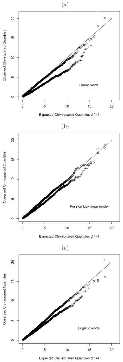
Quantile-quantile plots for the bootstrap χ² test statistics with sample size n = 100 and K = 5 (“circle” representing the proposed ${\chi }_{(K-1)}^2$ statistics based on the bootstrap sample MLE, and “+” representing the classical Pearson statistics based on the original data MLE): (a) the linear regression model; (b) the Poisson log-linear model; and (c) the logistic model.

We further examined the power of the proposed bootstrap χ² test by simulating data from the alternative hypothesis. Under the linear model, we simulated the error terms from a student t₍₂₎ distribution with two degrees of freedom, i.e., ∊ ~ t₍₂₎ in model (3.1). The covariates were generated similarly to those in the null case. We took the number of partitions K = 5, the sample size n = 150, and conducted 1,000 simulations. Under the linear model with the t₍₂₎ error, the power of our χ² test was 0.893. In another simulation with the linear model, we generated data from an alternative model with an extra quadratic term of covariate Z₁, that is,

$$y={\beta }_0+{\beta }_1{Z}_1+{\beta }_2{Z}_2+\gamma Z_1^2+∊,$$

while the null model is still given by (3.1). The power of the proposed χ² test was 0.817 for γ = 0.15, and 0.940 for γ = 0.2.

Similarly, for the Poisson regression model, we added an extra quadratic term in the Poisson mean function under the alternative model, that is,

$$\mu =\exp ({\beta }_0+{\beta }_1{Z}_1+{\beta }_2{Z}_2+\gamma Z_1^2).$$

If γ = 0.5, the power of our χ² test was 0.829, and if γ = 0.6, the power increased to 0.962. We also examined the case where the alternative model was from a negative binomial distribution but with the same mean as that of the Poisson mean. In particular, we took the mean of the negative binomial distribution μ = exp(β₀ +β₁Z₁ +β₂Z₂) and the negative binomial parameter p = r/(r +μ). The probability mass function of the negative binomial distribution is given by

$$P(x\mid p,r)=\left(\begin{array}{c}\hfill r+x-1\hfill \\ \hfill x\hfill \end{array}\right)p^r{(1-p)}^x,x=0,1,2,...,$$

which converges to a Poisson distribution (the null model), as r → ∞. When r = 0.7, the power of our chi-squared test was 0.838, and when r = 0.8, the corresponding power was 0.783.

Finally, we examined the test power for the logistic regression model using the proposed χ² test. Under the alternative hypothesis, we added a quadratic term in the logistic model,

$$p=\frac{\exp ({\beta }_0+{\beta }_1{Z}_1+{\beta }_2{Z}_2+\gamma Z_1^2)}{1+\exp ({\beta }_0+{\beta }_1{Z}_1+{\beta }_2{Z}_2+\gamma Z_1^2)},$$

where Z₁ was simulated from a uniform distribution on (1, 2) and Z₂ was still a binary covariate. As γ = 0 corresponded to the null model, we took γ = 0.4 to yield a power of 0.897 for our test, and γ = 0.5 to have a power of 0.976. We also examined a different modeling structure by taking p = Ψ(β₀ + β₁Z₁ + β₂Z₂), where Ψ(·) is the cumulative distribution function of an exponential distribution. Under this alternative, the power of the proposed test was 0.929. Our test uses the bootstrap data MLE, which recovers the chi-squared distribution. In contrast, the Chernoff and Lehmann test statistic does not follow any explicit distribution.

3.2. Application

As an illustration, we applied the proposed goodness-of-fit test to a well-known steam data set described in Draper and Smith (1998). The steam study contained n = 25 observations measured at intervals from a steam plant. The outcome variable was the monthly use of steam, and the covariates of interest included the operating days per month and the average atmospheric temperature. The steam data set was analyzed using a linear regression model, which involved three unknown regression parameters and the variance of the errors. The linear model was claimed to be of adequate fit based on the plot of residuals versus the predicted outcomes. This was also confirmed by the Durbin-Watson test (Draper and Smith, 1998).

To quantify the model fit in a more objective way, we applied the proposed bootstrap χ² test to examine how well the linear model fit the data from the steam study. Because the sample size was quite small, we partitioned the range of [0, 1] into 3 or 4 intervals, i.e., K = 3 or 4. We took 10,000 bootstrap samples from the original data, and for each of them, we computed the MLEs of the model parameters. Based on these MLEs, we constructed our ${\chi }_{(K-1)}^2$ test statistics by plugging the bootstrap sample MLEs in the Pearson-type statistic. In Figure 2, we show the histograms of the proposed ${\chi }_{\left(2\right)}^2$ and ${\chi }_{\left(3\right)}^2$ statistics for K = 3 and 4, respectively. We can see that among 10,000 bootstrap χ² test statistics only 2.92% of the test statistics exceed the critical value at the significance level of α = 0.05 for K = 3, while 2.75% for K = 4. Our findings provided strong evidence for the model fit, and thus confirmed that the linear regression model adequately fit the steam data.

Fig 2.

Histograms of the Pearson-type goodness-of-fit test statistics for the steam data with (a) K = 3 and (b) K = 4.

4. Discussion

We have proposed a bootstrap-based modification to the classical Pearson χ² goodness-of-fit test for regression models, which is a major extension of the work of Chernoff and Lehmann (1954) and Johnson (2004). The new procedure replaces the classical MLE from the original data by the MLE from a bootstrap sample. Using the MLE of a bootstrap sample adjusts the right amount of randomness to the test statistic. Not only does the proposed method restore the degrees of freedom, but also the χ² distribution itself, which would have been a nonstandard distribution lying between two χ² distributions with different degrees of freedom. Our simulation studies have shown that the proposed test statistic performs well with small sample sizes, and increasingly so as the sample size increases.

Compared with the well-known Akaike information criterion (AIC) and Bayesian information criterion (BIC), we may use the averaged value of the chi-squared statistics computed from a large number of bootstrap samples for model selection or comparison. A smaller value of the averaged chi-squared statistic indicates a better fitting model. It is worth noting that there is no scale associated with the AIC and BIC statistics, thus they are not meaningful alone. In other words, the AIC and the BIC by themselves do not provide any information on the goodness-of-fit of a single model, and they are only interpretable when comparing two or more competing models. In contrast, not only can our averaged bootstrap χ² statistic be used for model comparison or model selection, but also it is closely related to the χ² distribution, and as an approximation, one would know how well a model fits the data based on the corresponding χ² distribution. That is, the proposed test can be used for both model diagnostic and model selection at the same time. For example, a very large value of the averaged ${\chi }_{K-1}^2$ value for a small K may shed doubt on the model fit.

For the i.i.d. data, the minimum χ² statistic estimates the unknown parameter β by minimizing the χ² statistic or maximizing the grouped-data likelihood (Cramér, 1946). The minimum χ² statistic may not be directly applicable in regression settings due to difficulties involved in grouping the data with regression models. Also, it is challenging to generalize the proposed bootstrap Pearson-type statistic to censored data with commonly used semiparametric Cox proportional hazards model in survival analysis (Cox, 1972; Akritas, 1988; and Akritas and Torbeyns, 1997). Future research is warranted along these directions.

Appendix A: Proof of Theorem 2.1

We assume the conditions (a)-(d) in Cramér (1946, pp. 426-427), and the regularity conditions in Chernoff and Lehmann (1954, p. 581). The conditions in Cramér (1946) are sufficient to prove the χ² distribution when using the grouped data MLE. We essentially require the likelihood to be a smooth function of the parameter, the information in the sample increases with the sample size, and the third-order (partial) derivatives of the density function exist. Let β₀ be the true value of the parameter β, let $\widehat{\beta }$ be the MLE of β based on the original observations, and let β* be the MLE of β based on the bootstrap sample. Denote

$${\widehat{m}}_k=\sum _{i=1}^{n}I\{s_{k-1}\le F_{\widehat{\beta }}(y_i\mid Z_i)<s_k\},$$

$$m_k^{\ast }=\sum _{i=1}^{n}I\{s_{k-1}\le F_{\beta }\ast (y_i\mid Z_i)<s_k\},$$

$$m_k=\sum _{i=1}^{n}I\{s_{k-1}\le F_{{\beta }_0}(y_i\mid Z_i)<s_k\}.$$

Let $G(\alpha ,\gamma ,s)=E\left[F_{\gamma }\right\{F_{\alpha }^{-1}(s\mid Z_i)\mid Z_i\left\}\right]$, define ${\widehat{s}}_k=G({\beta }_0,\widehat{\beta },s_k)$, $t_k=G(\widehat{\beta },{\beta }_0,s_k)$, $r_k=G({\beta }^{\ast },{\beta }_0,s_k)$, ${\widehat{p}}_k={\widehat{s}}_k-{\widehat{s}}_{k-1}$, and b_k = t_k − t_k−1.

We have that

$$\frac{m_k^{\ast }-n{p}_k}{\sqrt{n{p}_k}}=\frac{m_k^{\ast }-{\widehat{m}}_k}{\sqrt{n{p}_k}}+\frac{{\widehat{m}}_k-m_k}{\sqrt{n{p}_k}}+\frac{m_k-n{p}_k}{\sqrt{n{p}_k}}.$$ (A.1)

If we follow the notation of (5) in Chernoff and Lehmann (1954), then $(m_k-{\mathit{np}}_k)∕\sqrt{{\mathit{np}}_k}={∊}_k$. We first analyze the term $({\widehat{m}}_k-m_k)∕\sqrt{{\mathit{np}}_k}$, by writing

$$\begin{array}{cc}\hfill & \frac{{\widehat{m}}_k-m_k}{\sqrt{n}}\hfill \\ \hfill =& \frac{1}{\sqrt{n}}\sum _{i=1}^n[I\left\{s_{k-1}\le F_{\widehat{\beta }}(y_i\mid Z_i)<s_k\right\}-[I\left\{s_{k-1}\le F_{{\widehat{\beta }}_0}(y_i\mid Z_i)<s_k\right\}]\hfill \\ \hfill =& \sqrt{n}[EI\left\{s_{k-1}\le F_{\widehat{\beta }}(y_i\mid Z_i)<s_k\right\}-EI\left\{s_{k-1}\le F_{{\widehat{\beta }}_0}(y_i\mid Z_i)<s_k\right\}]\hfill \\ \hfill & +O_p\left(n^{-1∕2}\right).\hfill \end{array}$$

The remaining term is of the same order as the standard deviation of $I\{s_{k-1}\le F_{\widehat{\beta }}(y_i\mid Z_i)<s_k\}-I\{s_{k-1}\le F_{{\beta }_0}(y_i\mid Z_i)<s_k\}$, which takes the value of 0 with probability $1-O(\widehat{\beta }-{\beta }_0)$, and the value of 1 or −1 with probability $O(\widehat{\beta }-{\beta }_0)=O_p\left(n^{-1∕2}\right)$. Thus, we can further write

$$\begin{array}{cc}\hfill & \frac{{\widehat{m}}_k-m_k}{\sqrt{n}}\hfill \\ \hfill =& \sqrt{n}\left[\mathrm{Pr}\left\{F_{\widehat{\beta }}(y_i\mid Z_i)<s_k\right\}-\mathrm{Pr}\left\{F_{\widehat{\beta }}(y_i\mid Z_i)<s_{k-1}\right\}-\mathrm{Pr}\left\{F_{{\beta }_0}(y_i\mid Z_i)<s_k\right\}+\mathrm{Pr}\left\{F_{{\beta }_0}(y_i\mid Z_i)<s_{k-1}\right\}\right]+O_p\left(n^{-1∕2}\right)\hfill \\ \hfill =& \sqrt{n}\left(\mathrm{Pr}\left[F_{{\beta }_0}(y_i\mid z_i)<F_{{\beta }_0}\left\{{F_{\widehat{\beta }}}^{-1}(s_k\mid Z_i)\mid Z_i\right\}\right]-\mathrm{Pr}\left[F_{{\beta }_0}(y_i\mid z_i)<F_{{\beta }_0}\left\{{F_{\widehat{\beta }}}^{-1}(s_k\mid Z_i)\mid Z_i\right\}\right]-s_k+s_{k-1}\right)+O_p\left(n^{-1∕2}\right)\hfill \\ \hfill =& \sqrt{n}(t_k-t_{k-1}-s_k+s_{k-1})=O_p\left(n^{-1∕2}\right)\hfill \\ \hfill =& \sqrt{n}(b_k-p_k)+O_p\left(n^{-1∕2}\right).\hfill \end{array}$$

We now show that b_k−p_k can be approximated by $p_k-{\widehat{p}}_k$, in the classical MLE construction. Note that $s_k=G({\beta }_0,{\beta }_0,s_k)=G(\widehat{\beta },\widehat{\beta },s_k)$. Denoting

$$G_1(\alpha ,\gamma ,s)=\frac{\partial G(\alpha ,\gamma ,s)}{\partial \alpha },G_2(\alpha ,\gamma ,s)=\frac{{\partial }^{2}G(\alpha ,\gamma ,s)}{\partial \alpha \partial {\gamma }^T},$$

we have that

$$\begin{array}{cc}\hfill & (b_k-p_k)-(p_k-{\widehat{p}}_k)\hfill \\ \hfill =& G(\widehat{\beta },{\beta }_0,s_k)-G(\widehat{\beta },{\beta }_0,s_{k-1})-G({\beta }_0,{\beta }_0,s_k)+G({\beta }_0,{\beta }_0,s_{k-1})-G(\widehat{\beta },\widehat{\beta },s_k)+G(\widehat{\beta },\widehat{\beta },s_{k-1})+G({\beta }_0,\widehat{\beta },s_k)-G({\beta }_0,\widehat{\beta },s_{k-1})\hfill \\ \hfill =& G_1{({\beta }_0,{\beta }_0,s_k)}^T(\widehat{\beta }-{\beta }_0)-G_1{({\beta }_0,{\beta }_0,s_{k-1})}^T(\widehat{\beta }-{\beta }_0)-G_1{({\beta }_0,\widehat{\beta },s_k)}^T(\widehat{\beta }-{\beta }_0)+G_1{({\beta }_0,\widehat{\beta },s_{k-1})}^T(\widehat{\beta }-{\beta }_0+O_p(n^{-1})\hfill \\ \hfill =& -{(\widehat{\beta }-{\beta }_0)}^T{G}_2({\beta }_0,{\beta }_0,s_k)(\widehat{\beta }-{\beta }_0)+{(\widehat{\beta }-{\beta }_0)}^T{G}_2({\beta }_0,{\beta }_0,s_{k-1})(\widehat{\beta }-{\beta }_0)+O_p\left(n^{-1}\right)\hfill \\ \hfill =& O_p\left(n^{-1}\right).\hfill \end{array}$$

Thus, $\sqrt{n}(b_k-p_k)=\sqrt{n}(p_k-{\widehat{p}}_k)+O_p\left(n^{-1∕2}\right)$, and

$$\frac{{\widehat{m}}_k-m_k}{\sqrt{npk}}=\frac{n(p_k-{\widehat{p}}_k)}{\sqrt{npk}}+o_p\left(1\right)=-{\widehat{v}}_k+o_p\left(1\right),$$

where ${\widehat{v}}_k$ is defined in (7) of Chernoff and Lehmann (1954).

We now consider the first term in (A.1). Following the bootstrap principle, the conditional distribution of this term should be the same as that of the second one. We show that in fact the two terms are identically distributed as n → ∞, and they are independent. As an intermediate result, we have already established that

$$\frac{{\widehat{m}}_k-m_k}{\sqrt{n}}={\left\{G_1\right({\beta }_0,{\beta }_0,s_k)-G_1({\beta }_0,{\beta }_0,s_{k-1}\left)\right\}}^T\sqrt{n}(\widehat{\beta }-{\beta }_0)+o_p\left(1\right).$$

Following a similar derivation, we have that

$$\begin{array}{cc}\hfill & \frac{m_k^{\ast }-{\widehat{m}}_k}{\sqrt{n}}\hfill \\ \hfill =& \frac{1}{\sqrt{n}}\sum _{i=1}^n\left[I\{s_{k-1}\le F_{{\beta }^{\ast }}(y_i\mid Z_i)<s_k\}-I\{s_{k-1}\le F_{\widehat{\beta }}(y_i\mid Z_i)<s_k\}\right]\hfill \\ \hfill =& \sqrt{n}\left[EI\{s_{k-1}\le F_{{\beta }_{\ast }}(y_i\mid Z_i<s_k\}-EI\{s_{k-1}\le F_{\widehat{\beta }}(y_i\mid Z_i)<s_k\}\right]+O_p\left(n^{-1∕2}\right)\hfill \\ \hfill =& \sqrt{n}\left[\mathrm{Pr}\left\{F_{{\beta }^{\ast }}\right(y_i\mid Z_i)<s_k\}-\mathrm{Pr}\left\{F_{{\beta }^{\ast }}\right(y_i\mid Z_i)<s_{k-1}\}-\mathrm{Pr}\left\{F_{\widehat{\beta }}\right(y_i\mid Z_i)<s_k\}+\mathrm{Pr}\left\{F_{\widehat{\beta }}\right(y_i\mid Z_i)<s_{k-1}\}\right]+O_p\left(n^{-1∕2}\right)\hfill \\ \hfill =& \sqrt{n}\left[\mathrm{Pr}\left\{F_{{\beta }_0}\right(y_i\mid Z_i)<F_{{\beta }_0}\{F_{{\beta }^{\ast }}^{-1}(s_k\mid Z_i)\mid Z_i\}-\mathrm{Pr}\{F_{{\beta }_0}(y_i\mid Z_i)<F_{{\beta }_0}\left\{F_{{\beta }^{\ast }}^{-1}\right(s_{k-1}\mid Z_i)\mid Z_i\}-\mathrm{Pr}\left\{F_{{\beta }_0}\right(y_i\mid Z_i)<F_{{\beta }_0}\{F_{{\beta }^{\ast }}^{-1}(s_k\mid Z_i)\mid Z_i\}+\mathrm{Pr}\{F_{{\beta }_0}(y_i\mid Z_i)<F_{{\beta }_0}\left\{F_{{\beta }^{\ast }}^{-1}\right(s_{k-1}\mid Z_i)\mid Z_i\}\right]+O_p\left(n^{-1∕2}\right)\hfill \\ \hfill =& \sqrt{n}(r_k-r_{k-1}-t_k+t_{k-1})+O_p\left(n^{-1∕2}\right)\hfill \\ \hfill =& \sqrt{n}\left\{G\right({\beta }^{\ast },\beta ,s_k)-G({\beta }^{\ast },{\beta }_0,s_{k-1})-G(\widehat{\beta },{\beta }_0,s_k)+G(\widehat{\beta },{\beta }_0,s_{k-1}\left)\right\}+O_p\left(n^{-1∕2}\right)\hfill \\ \hfill =& \sqrt{n}\left\{G_1\right(\widehat{\beta },{\beta }_0,s_k\left)\right({\beta }^{\ast }-\widehat{\beta })-G_1(\widehat{\beta },{\beta }_0,s_{k-1}\left)\right({\beta }^{\ast }-\widehat{\beta }\left)\right\}+O_p\left(n^{-1∕2}\right)\hfill \\ \hfill =& \left\{G_1\right({\beta }_0,{\beta }_0,s_k)-G_1({\beta }_0,{\beta }_0,s_{k-1}\left)\right\}\sqrt{n}({\beta }^{\ast }-\widehat{\beta })+o_p\left(1\right).\hfill \end{array}$$

Note that G₁(β₀, β₀, s_k) − G₁(β₀, β₀, s_k−1) is a nonrandom quantity. As n → ∞, $\sqrt{n}(\widehat{\beta }-{\beta }_0)$ converges to a normal distribution with mean zero. Conditional on $\widehat{\beta }$, $\sqrt{n}({\beta }^{\ast }-\widehat{\beta })$ also converges to a mean zero normal distribution. In addition, $\sqrt{n}({\beta }^{\ast }-\widehat{\beta })$ and $\sqrt{n}(\widehat{\beta }-{\beta }_0)$ are asymptotically uncorrelated, so they are independent of each other asymptotically. Hence, we can represent the first term of (A.1) as $v_k^{\ast }+o_p\left(1\right)$, which is independent of ${\widehat{v}}_k$ and ∊k, and has the same distribution as ${\widehat{v}}_k$.

Let ∊ = (∊₁, … , ∊_K)^T, and similarly define $∊={({∊}_1,\dots ,{∊}_K)}^T$ and υ*. Now, following the notations and arguments of Chernoff and Lehmann (1954), we let the information matrix be $\tilde{J}=D^{T}D$, where D is the matrix with element $(\partial p_k∕\partial {\beta }_j)∕\sqrt{p_k}$ for j, k = 1, … , K. Note that ∊ ~ N(0, I − qq^T) asymptotically, where $q={(\sqrt{p_1},\dots ,\sqrt{p_K})}^T$,

$$\widehat{v}=D{(\tilde{J}+J^{\ast })}^{-1}{D}^T∊+D{(\tilde{J}+J^{\ast })}^{-1}\eta +o_p\left(1\right),$$

where η ~ N(0, J*), J* is defined the same as in Chernoff and Lehmann (1954, p. 583), and η is independent of ∊. We use e and τ to denote random variables that have the same distributions as ∊ and η, respectively. Note that ∊, η, e and τ are all independent of each other. We then have that

$$\begin{array}{cc}\hfill & {\left(\frac{m_1^{\ast }-np1}{\sqrt{np1}},\dots ,\frac{m_K^{\ast }-npK}{\sqrt{npK}}\right)}^T\hfill \\ \hfill =& ∊-\widehat{v}-v^{\ast }+o_p\left(1\right)\hfill \\ \hfill =& ∊-D{(\tilde{J}+J^{\ast })}^{-1}{D}^T∊-D{(\tilde{J}+J^{\ast })}^{-1}\eta -D{(\tilde{J}+J^{\ast })}^{-1}{D}^{T}e-D{(\tilde{J}+J^{\ast })}^{-1}\tau +o_p\left(1\right)\hfill \\ \hfill =& \{I-D{(\tilde{J}+J^{\ast })}^{-1}{D}^T\}∊-D{(\tilde{J}+J^{\ast })}^{-1}\eta -D{(\tilde{J}+J^{\ast })}^{-1}{D}^{T}e-D{(\tilde{J}+J^{\ast })}^{-1}\tau +o_p\left(1\right).\hfill \end{array}$$

Note that D^T q = 0, var(η) = J* and $D^{T}D=\tilde{J}$. As n → ∞, (A.2) converges to a normal random vector with the variance-covariance matrix

$$\begin{array}{cc}\hfill & \{I-D{(\tilde{J}+J^{\ast })}^{-1}{D}^T\}(I-q{q}^T)\{I-D{(\tilde{J}+J^{\ast })}^{-1}{D}^T\}+D{(\tilde{J}+J^{\ast })}^{-1}{J}^{\ast }{(\tilde{J}+J^{\ast })}^{-1}{D}^T+D{(\tilde{J}+J^{\ast })}^{-1}{D}^T(I-q{q}^T)D{(\tilde{J}+J^{\ast })}^{-1}{D}^T+D{(\tilde{J}+J^{\ast })}^{-1}{J}^{\ast }{(\tilde{J}+J^{\ast })}^{-1}{D}^T\hfill \\ \hfill =& I-q{q}^T-2D{(\tilde{J}+J^{\ast })}^{-1}{D}^T+2D{(\tilde{J}+J^{\ast })}^{-1}{J}^{\ast }{(\tilde{J}+J^{\ast })}^{-1}{D}^T+2D{(\tilde{J}+J^{\ast })}^{-1}\tilde{J}{(\tilde{J}+J^{\ast })}^{-1}{D}^T\hfill \\ \hfill =& I-q{q}^T,\hfill \end{array}$$

which is the same as the asymptotic variance-covariance matrix of ∊. This completes the proof that Q^Boot(β*) has a ${\chi }_{(K-1)}^2$ distribution as n → ∞.

References

- Akaike H. Information theory and an extension of the maximum likelihood principle. In: Petrov BN, Csaki F, editors. Second International Symposium on Information Theory. Akademiai Kiado; Budapest: 1973. pp. 267–281. MR0483125. [Google Scholar]
- Akritas MG. Pearson-type goodness-of-fit tests: the univariate case. Journal of the American Statistical Association. 1988;83:222–230. MR0941019. [Google Scholar]
- Akritas MG, Torbeyns AF. Pearson-type goodness-of-fit tests for regression. The Canadian Journal of Statistics. 1997;25:359–374. MR1486917. [Google Scholar]
- Ali MM. An approximation to the null distribution and power of the Durbin-Watson statistic. Biometrika. 1984;71:253–261. MR0767153. [Google Scholar]
- Chernoff H, Lehmann EL. The use of maximum likelihood estimates in χ2 tests for goodness of fit. Annals of Mathematical Statistics. 1954;25:579–586. MR0065109. [Google Scholar]
- Claeskens G, Hjort LN. Model Selection and Model Averaging. Cambridge University Press; 2008. MR2431297. [Google Scholar]
- Cox DR. Regression models and life-tables (with discussion) Journal of the Royal Statistical Society, Series B. 1972;34:187–220. MR0341758. [Google Scholar]
- Cramér H. Mathematical Methods of Statistics. Princeton University Press; 1946. MR0016588. [Google Scholar]
- Draper NR, Smith H. Applied Regression Analysis. 3rd edition. John Wiley & Sons; New York: 1998. MR1614335. [Google Scholar]
- Durbin J. Distribution Theory for Tests Based on the Sample Distribution Function. Philadelphia: 1973. SIAM Publications No. 9. MR0305507. [Google Scholar]
- Imhof JP. Computing the distribution of quadratic forms in normal variables. Biometrika. 1961;48:419–426. MR0137199. [Google Scholar]
- Johnson VE. A Bayesian χ2 test for goodness-of-fit. The Annals of Statistics. 2004;32:2361–2384. MR2153988. [Google Scholar]
- Johnson VE. Bayesian model assessment using pivotal quantities. Bayesian Analysis. 2007;2:719–734. MR2361972. [Google Scholar]
- McCullagh P, Nelder JA. Generalized Linear Models. 2nd edition. Chapman and Hall; London: 1989. MR0727836. [Google Scholar]
- Pearson K. On the criterion that a given system of deviations from the probable in the case of a correlated system of variables is such that it can be reasonably supposed to have arisen from random sampling. Philosophical Magazine. 1900;50:157–175. [Google Scholar]
- Stephens MA. On the half-sample method for goodness-of-fit. Journal of the Royal Statistical Society, Series B. 1978;40:64–70. [Google Scholar]
- Stute W, Zhu L-X. Model checks for generalized linear models. Scandinavian Journal of Statistics. 2002;29:535–545. MR1925573. [Google Scholar]
- Stute W, Manteiga GW, Quindimilm PM. Bootstrap approximations in model checks for regression. Journal of the American Statistical Association. 1998;93:141–149. MR1614600. [Google Scholar]
- Su JQ, Wei LJ. A lack-of-fit test for the mean function in a generalized linear model. Journal of the American Statistical Association. 1991;86:420–426. MR1137124. [Google Scholar]