Diverse Visual Features Encoded in Mouse Lateral Geniculate Nucleus

Abstract

The thalamus is crucial in determining the sensory information conveyed to cortex. In the visual system, the thalamic lateral geniculate nucleus (LGN) is generally thought to encode simple center-surround receptive fields, which are combined into more sophisticated features in cortex, such as orientation and direction selectivity. However, recent evidence suggests that a more diverse set of retinal ganglion cells projects to the LGN. We therefore used multisite extracellular recordings to define the repertoire of visual features represented in the LGN of mouse, an emerging model for visual processing. In addition to center-surround cells, we discovered a substantial population with more selective coding properties, including direction and orientation selectivity, as well as neurons that signal absence of contrast in a visual scene. The direction and orientation selective neurons were enriched in regions that match the termination zones of direction selective ganglion cells from the retina, suggesting a source for their tuning. Together, these data demonstrate that the mouse LGN contains a far more elaborate representation of the visual scene than current models posit. These findings should therefore have a significant impact on our understanding of the computations performed in mouse visual cortex.

Introduction

The retina parses the visual scene into a set of features that are conveyed to the central visual system. At each stage, the visual scene representation can be transformed to extract new features. The textbook example of this, described by Hubel and Wiesel (Hubel and Wiesel, 1962), is the transformation from circular center-surround receptive fields (RFs) in the lateral geniculate nucleus (LGN) to selectivity for bars or edges of a specific orientation in primary visual cortex (V1). A hallmark of this standard model is that the only information available to V1 from subcortical relays is a set of simple ON and OFF circular RFs, and that other properties are computed anew in V1. Understanding the full array of visual features delivered to V1 is therefore crucial in understanding its function (Hirsch and Martinez, 2006).

Evidence has accumulated that there may be more diversity in the signals sent to LGN than generally appreciated (Field and Chichilnisky, 2007; Masland and Martin, 2007). First, a number of more complex operations than simple center-surround have been described in the retina of rodents and rabbits, including direction selectivity, local edge detectors, and sensitivity to differential motion (Gollisch and Meister, 2010). Until recently, it was thought that many of these cell types may not project to LGN; however, genetic methods in mouse have shown that direction-selective (DS) retinal ganglion cells (RGCs) provide monosynaptic inputs to the LGN (Huberman et al., 2009; Kay et al., 2011; Rivlin-Etzion et al., 2011), and retrograde tracing studies in primate have shown at least seven morphologically distinct RGC types that project to LGN (Dacey et al., 2003). Together, these findings raise the strong possibility that diverse visual features may arrive in the LGN.

We chose to investigate LGN response properties in the mouse, which has recently emerged as a prominent model system to study visual processing (Hubener, 2003; Huberman and Niell, 2011). A number of studies have begun to investigate the computations performed in visual cortex (Niell and Stryker, 2008; Liu et al., 2011; Atallah et al., 2012; Lee et al., 2012; Olsen et al., 2012; Wilson et al., 2012). However, despite the importance of knowing the inputs from LGN to understand cortical computation (Gao et al., 2010), few studies have recorded from mouse LGN (Cang et al., 2008; Niell and Stryker, 2010; Olsen et al., 2012), and to date only one study has performed a dedicated characterization of RF properties (Grubb and Thompson, 2003). That study confirmed that basic LGN properties are similar in the mouse and other species, in particular the center-surround organization of the standard model. However, this survey depended on a white-noise mapping procedure, which can fail to capture many nonlinear response types. A recent publication used in vivo calcium imaging to characterize direction tuning of LGN neurons but was limited to the superficial-most 75 μm of LGN (Marshel et al., 2012). Thus, the vast majority of the mouse LGN, both in terms of volume and response types, has remained physiologically uncharacterized.

We therefore used multisite extracellular recordings and applied a broad set of visual stimuli to characterize the complete repertoire of visual responses throughout the mouse LGN. Given the small size of the mouse brain, it was feasible to thoroughly sample the full extent of the LGN with a moderate number of recordings and thus avoid missing any cell types that might be localized to specific subregions, or that exist at relatively low overall numbers. Post hoc reconstruction of recording sites across multiple experiments allowed us to determine the 3D organization and to correlate this with anatomical and genetic markers.

Our study, along with the recent work of Marshel et al. (2012), shows that mouse LGN does not only convey the standard center-surround pathways. We demonstrate the encoding of diverse features, including orientation and direction selectivity along the four cardinal axes, and cells suppressed by contrast. Furthermore, the orientation and direction-selective LGN neurons displayed regional biases that were matched to incoming direction tuned retinal afferents, supporting a mechanism for their tuning based on both inheritance and pooling of retinal inputs.

Materials and Methods

Mice.

Animals were maintained in the animal facility at University of Oregon or the University of California, San Diego and used in accordance with protocols approved by the University of California, San Diego and University of Oregon Institutional Animal Care and Use Committees.

Extracellular multisite electrophysiology.

Electrophysiological recordings were performed on adult C57Bl/6 mice (age 2–4 months, both male and female). Recordings were performed generally as described previously (Cang et al., 2008), except for a change from urethane to isoflurane anesthesia, which eliminated the need for a tracheotomy and provides a more stable anesthetized state than an injectable agent. We performed these recordings under anesthesia, rather than a previous head-fixed awake paradigm (Niell and Stryker, 2010), to facilitate the presentation of a large stimulus set for complete characterization of the population. Previous studies in mouse cortex (Niell and Stryker, 2010; Andermann et al., 2011) have indicated that, although firing rates can change, particularly with behavioral state, tuning properties in V1 are generally similar in awake and anesthetized recordings, and one would expect this to be further true one synapse upstream in the thalamus. However, future studies focused more closely on particular response properties could investigate the effect of anesthesia and behavioral state on retinogeniculate processing.

In preparation for recording, mice were anesthetized with a surgical level of isoflurane (4% induction, 2% maintenance, in O₂), and body temperature was maintained at 37.5°C by a feedback-controlled heating pad. After a scalp incision, the fascia was cleared from the surface of the skull, and a metal headplate was affixed to the skull with vetbond and dental acrylic (Niell and Stryker, 2010). The headplate provided stability for mounting the mouse, and an opening to allow access to the skull. A craniotomy of ∼2 mm in diameter was performed over the LGN, at 2.5 mm lateral and 2.0 mm anterior to the lambda suture. The exposed cortical surface was covered with 2% agarose in 0.9% saline to prevent drying and provide mechanical support.

At this point, the mouse was transferred to the recording setup, and a dose of chlorprothixene (0.5 mg/kg) was administered intraperitoneally. Administration of chlorprothixene allowed us to lower isoflurane levels to 0.6%, which gave robust visual responses while maintaining an anesthetized state (Kaneko et al., 2008). Recordings were made with silicon multisite electrodes (a1×32–25-5 mm-177, NeuroNexus Technologies), which were coated with a small amount of the lipophilic vital dye DiI or DiO (Invitrogen). The electrode was inserted through the craniotomy and overlying agarose using a microdrive (Siskiyou Designs), and lowered down to the LGN. At a depth of ∼2500–3000 μm, the LGN could be identified by rapid firing in response to either ON or OFF flashes of a small spot at a specific location in the visual field. Beyond localizing to the LGN, the electrode was placed without regard for the presence of responsive units on individual sites, and all units stably isolated over the recording period were included in analysis. Upon locating the LGN, the electrode was further embedded in agarose to increase mechanical stability, and the electrode was allowed to settle in one position for 30 min to obtain stable single-unit recordings. The eyes were covered with ophthalmic ointment until recording, at which time the eyes were rinsed with saline and a thin layer of silicone oil (30,000 centistokes) was applied to prevent drying while allowing clear optical transmission.

At the end of recording, the animal was killed under deep anesthesia by cervical dislocation. The brain was removed immediately and fixed by immersion in 4% paraformaldehyde in PBS at 4°C overnight, after which 200 μm coronal sections were cut with a vibratome. The sections were mounted using Vectashield with DAPI (Vector Laboratories) and imaged on an Olympus BX6l microscope with 2× and 20× air objectives and DP72 camera, to reconstruct electrode penetrations in the LGN.

Data acquisition.

Data acquisition was performed as described by Niell and Stryker (2008). Signals were acquired using a System 3 workstation (Tucker-Davis Technologies) and analyzed with custom software in Matlab (MathWorks). To obtain single-unit activity, the extracellular signal was filtered from 0.7 to 7 kHz and sampled at 25 kHz. Spiking events were detected on-line by voltage threshold crossing, and a 1 ms waveform sample on 4 neighboring recording sites was acquired around the time of threshold crossing. Single-unit clustering and spike waveform analysis were performed as described previously (Niell and Stryker, 2008), with a combination of custom software in Matlab and Klusta-Kwik (Harris et al., 2000). Quality of separation was determined based on the Mahalanobis distance and L-ratio (Schmitzer-Torbert et al., 2005) and evidence of a clear refractory period. Units were also checked for stability in terms of amplitude and waveform over the course of the recording time to ensure that they had not drifted or suffered mechanical damage. Units that were found by histology to be outside the LGN, generally above or below resulting from the length of the electrode, were excluded from subsequent analysis.

Visual stimuli.

Visual stimuli were presented as described previously (Niell and Stryker, 2008). Briefly, stimuli were generated in Matlab using the Psychophysics Toolbox extensions (Brainard, 1997; Pelli, 1997) and displayed with gamma correction on a monitor (Planar SA2311W, 30 × 50 cm, 60 Hz refresh rate) placed 25 cm from the mouse, subtending ∼60–75° of visual space. The monitor was placed either centered directly in front of the mouse or offset to 45° and raised or lowered up to 10 cm, depending on the hand-mapped RF location of multiunit activity. To probe for a broad range of visual response types across an ensemble of simultaneously recorded units, we used a battery of stimuli meant to measure response parameters typically assessed in retina, LGN, and V1, as shown in Figure 1D–G.

Figure 1.

Multisite recording of visual response properties in mouse LGN. A, Schematic of 32-site silicon probe used for recordings. B, Reconstruction of electrode track in LGN. Blue, DAPI; green, DiO. C, RFs of eight units simultaneously recorded (of 14 total) from recording shown in B. There is retinotopic organization along the length of the electrode, as RFs move from top of visual field to bottom. D–G, Four stimulus sets used for visual response characterization. D, Contrast modulated band-limited noise. E, Drifting sinusoidal gratings. F, Flashing spots. G, Moving spots.

Drifting sinusoidal gratings were presented at eight evenly spaced directions of motion, with temporal frequency of 2 and 8 Hz, and spatial frequency of 0.01, 0.02, 0.04, 0.08, 0.16, and 0.32 cpd, plus full-field flicker (0 cpd). Stimuli were randomly interleaved and presented for 1 s duration, with 0.1 s interstimulus interval. A gray blank condition (mean luminance) was included to estimate the spontaneous firing rate.

Contrast-modulated noise movies (Niell and Stryker, 2008) were created by first generating a random spatiotemporal frequency spectrum in the Fourier domain with defined spectral characteristics. To drive as many simultaneously recorded units as possible, we used a spatial frequency spectrum that dropped off as A(f) ∼ 1/(f + f_c), with f_c = 0.05 cpd, and a sharp cutoff at 0.16 cpd, to approximately match the stimulus energy to the distribution of spatial frequency preferences. The temporal frequency spectrum was flat with a sharp low-pass cutoff at 10 Hz. This 3D (ω_x, ω_y, ω_t) spectrum was then inverted to generate a spatiotemporal movie. To provide contrast modulation, this movie was multiplied by a sinusoidally varying contrast with 10 s period. Each movie was 5 min long and was repeated two or three times, for 10–15 min total presentation.

Sparse flashing noise consisted of ON (full luminance) and OFF (minimum luminance) circular spots on a gray background, at a density such that on average 15% of the area on the screen was covered on any given frame. Spots were 2, 4, 8,16, and 32° in diameter, and presented such that each size made up an equal fraction of the area on the screen (e.g., number of spots was inversely proportional to their area), to ensure even coverage at each point in space by every size. In addition, 20 frames each of full-screen ON and OFF were randomly interleaved. Each movie frame was presented for 250 ms followed by immediate transition to the next frame, for a total duration of 10 min.

A sparse moving noise stimulus was generated, also using ON and OFF spots, with a more limited size range (4, 8, 16° diameter), but each spot was assigned to move in one of eight evenly spaced directions and one of 5 speeds (10, 20, 40, 80, 160°/s). Spots appeared on the appropriate edge of the screen and moved across until they disappeared on the far edge. The movie was presented for 20 min total duration. Although we hoped that this stimulus would give a second measure of direction selectivity, the direction tuning curves were not very robust, although size and speed tuning were. In retrospect, this is likely because we used circular spots, so that the edge is not always perpendicular to the direction of movement as it is for a bar or grating. Combined with the fact that stimuli were not controlled to pass directly over the center of a given neuron's RF (because of parallel recording), this would lead to a range of apparent directions resulting from the aperture effect, whereby only the component of motion perpendicular to a contour can be detected when observed through a limited spatial window (Marr and Ullman, 1981).

Data analysis.

Data analysis was performed using custom routines written in Matlab. Statistical significance was determined by Mann–Whitney U test, except where otherwise stated. For figures representing the median of data, error bars indicate SE of the median as calculated by a bootstrap. In other cases, error bars indicate SEM.

Neurons in LGN can respond to a drifting grating with either an increase in mean firing rate, or by a modulation of firing up and down around the spontaneous rate, with the latter indicative of a purely linear response. We therefore calculated tuning curves for the drifting sinusoidal gratings using the mean evoked F0 (total firing rate) and F1 (modulation at grating temporal frequency) responses across trials for each stimulus condition, with the measured spontaneous rate for blank trials subtracted. We found that the F0 and F1 generally agreed for neurons with a strong F1 response, so subsequent tuning analysis was based on the F0 response. Spatial frequency tuning was computed using the mean response across all orientations and orientation selectivity at the spatial frequency that gave the largest response. F1/F0 ratio for a unit was the ratio of the average F1 and F0 response at this spatial frequency. We presented two different temporal frequencies (TFs), 2 and 8 Hz, and computed the temporal frequency preferences as (R_hi − R_low)/(R_hi + R_low), with R_hi and R_low being the peak firing rates at each temporal frequency, for an index where −1 indicates only low TF response, +1 only high TF response, and 0 representing equal response to both.

Orientation and direction selectivity indices (OSI/DSI) and preference were computed from these tuning curves using a standard metric based on the circular variance, which consists of a vector sum of the responses across orientations given as follows:

The absolute amplitude of this value gives the index, whereas the complex phase (or half the complex phase for OSI) gives the preferred orientation/direction. This index provides a global measure of tuning, which takes into account both tuning width and depth of modulation in a single index for the clustering algorithm, and proved more robust than curve-fitting for tuning curves that are not densely sampled.

To analyze the response to contrast-modulated white-noise movies, we binned the number of spikes in response to each frame of the movie. The spatiotemporal spike-triggered average (STA) of contrast-modulated movie responses was computed by the mean of the frames at a range of temporal offsets before each spike. Because we used a 1/f power spectrum for the stimulus set, the raw STA is broadened by the correlations in the stimulus set. However, because the stimulus is Gaussian and therefore only contains second-order correlations, we were able to correct the STA by normalizing its Fourier transform by the power spectrum of the stimulus set (Sharpee et al., 2004). Although this can account for the under-represented high spatial frequencies, it cannot recover frequencies excluded from the stimulus (>0.16 cpd and 10 Hz).

We used singular value decomposition to separate the joint spatiotemporal RF into pairs of spatial and temporal components (Wolfe and Palmer, 1998). For all units with an evident response in the joint STA, this gave a spatial component with a clearly localized response, which was used as the spatial STA with the corresponding temporal STA. Units that did not have a spatial STA component with amplitude significantly above the noise background were left unclassified for spatial RF analysis. The spatial STA was then fit to a 2D Gaussian to determine RF center and amplitude. This fit cannot account for an opposing surround, as this would require a fit to a difference of two Gaussians, which would be less robust. However, our fits were clearly sufficient for determining RF location and polarity, and for providing a measure of RF center size. The temporal STA was used to assess how biphasic the response was, based on the ratio of the initial maximum or minimum (for ON and OFF, respectively) to the subsequent minimum or maximum.

To analyze sparse noise movies, we computed spiked-triggered averages for ON and OFF spots separately (to avoid averaging out ON/OFF responses in nonlinear units) and determined the RF location as the point with the largest absolute magnitude response across the two STAs. We computed peristimulus time histograms locked to the onset of each flashed spot that coincided with this location. Histograms were separated out based on polarity and size of the spot. The mean response during spot presentation (250 ms) was used to determine response amplitude as a function of polarity and size. For the preferred size and polarity, a measure of sustained response was generated as the ratio of the mean response during spot presentation to the peak response.

For moving spots, a similar analysis was followed except that responses were locked to the time a spot first crossed the RF point and were separated out by speed as well as size and polarity. The mean response throughout the time the spot was over the RF location was used to construct a speed tuning curve.

This analysis resulted in a set of response parameters for each unit (listed in Table 1). Each parameter was zero-centered and normalized to have unity variance across the population, and the resulting response profiles were used in a fuzzy k-means clustering algorithm (Matlab Central). We heuristically found that setting the fixed number of clusters to n = 6 achieved a tradeoff between poor correlations within clusters (too few clusters) and excessive splitting (too many clusters). Setting n = 5 merged the “slow” group into the DS/orientation-selective (OS) group and sON/sOFF groups, reducing the within-group correlations, and n = 7 split the “slow” group into new groups whose characteristic differences were not clear.

Table 1.

Median population values for response parameters used in clustering

	sON (n = 64)	sOFF (n = 28)	tOFF (n = 42)	DS/OS (n = 28)	Slow (n = 38)	Suppressed (n = 14)
STA RF amplitude	0.9 ± 0.02	−1.0 ± 0.03	−0.8 ± 0.06	0.2 ± 0.13	0.0 ± 0.13	NA
Flashed spot polarity	1.0 ± 0.03	−0.9 ± 0.07	−0.8 ± 0.10	0.1 ± 0.19	0.3 ± 0.16	NA
Biphasic index	0.3 ± 0.03	0.3 ± 0.03	0.6 ± 0.03	0.2 ± 0.05	0.3 ± 0.04	NA
Peak flash response latency (ms)	94.3 ± 4.99	92.6 ± 6.26	84.1 ± 4.38	142.3 ± 10.59	176.4 ± 7.63	NA
Preferred spot diameter (°)	11.6 ± 1.22	15.9 ± 2.83	14.0 ± 2.50	17.2 ± 3.66	17.3 ± 2.73	28.4 ± 6.70
Sustain index	0.6 ± 0.03	0.6 ± 0.03	0.4 ± 0.02	0.4 ± 0.03	0.6 ± 0.02	NA
Correlation of ON/OFF flash resp	−0.3 ± 0.05	−0.4 ± 0.05	−0.1 ± 0.06	−0.1 ± 0.08	0.3 ± 0.07	0.4 ± 0.14
Preferred speed (°/s)	109.5 ± 6.82	120.0 ± 8.89	110.6 ± 8.05	37.3 ± 4.65	33.4 ± 4.10	NA
Temporal frequency index	0.0 ± 0.04	−0.1 ± 0.06	0.1 ± 0.06	−0.3 ± 0.10	−0.5 ± 0.06	NA
Preferred spatial frequency (cpd)	0.05 ± 0.006	0.03 ± 0.003	0.02 ± 0.003	0.10 ± 0.019	0.06 ± 0.016	NA
Direction selectivity index (DSI)	0.1 ± 0.01	0.0 ± 0.02	0.1 ± 0.02	0.2 ± 0.05	0.1 ± 0.02	NA
Orientation selectivity index (OSI)	0.1 ± 0.01	0.1 ± 0.01	0.1 ± 0.02	0.6 ± 0.05	0.2 ± 0.01	NA
Linearity (F1/F0)	1.7 ± 0.06	1.8 ± 0.12	1.8 ± 0.13	1.0 ± 0.18	1.0 ± 0.10	NA
Evoked movie response (sp/s)	4.0 ± 0.51	4.6 ± 0.83	3.2 ± 0.60	1.4 ± 0.52	1.2 ± 0.24	−4.2 ± 2.59
Spontaneous firing rate (sp/s)	1.0 ± 0.28	1.7 ± 0.35	1.0 ± 0.35	1.7 ± 0.31	1.3 ± 0.21	8.3 ± 1.76

NA, Not applicable.

Histological reconstruction of recording sites.

To reconstruct the 3D functional organization of the LGN, we determined the location of each recorded unit and mapped it onto a common LGN template, using custom Matlab software. The outline of LGN and the electrode track from post hoc histology were manually traced. The boundaries of the LGN are readily visible from bright-field and autofluorescence of the histology brain tissue and from DAPI staining: the optic tract marks the dorsal and lateral LGN borders and a small but sharp gap in soma density marks the LGN′s medial and ventral borders; this gap represents the major site of afferent and efferent LGN fibers comprising the internal capsule and is invariant with respect to anterior–posterior position in the LGN (see Fig. 8, hyphenated line depicting this boundary).

Figure 8.

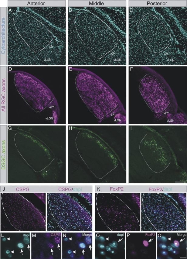
Distribution of direction-tuned retino-LGN axons and putative cell type-specific markers in the mouse LGN. A–C, DAPI-labeled nuclei (blue) in the anterior (A), middle (B), and posterior (C) LGN. Hyphenated lines display the boundaries of the LGN. D–F, RGC axons labeled with cholera toxin β conjugated to Alexa-594 (CTb-594), after injection into the vitreous of the eye. The axons fill the entire LGN (compare with A–C) as well as neighboring visual structures. G–I, Axon terminations of genetically labeled On-Off DS RGCs (green) in the lateral portion of the anterior (A), middle (B), and posterior (C) LGN. A relatively greater portion of the posterior LGN (C) contains DS inputs compared with more anterior aspects (A, B), which is consistent with the electrophysiological recordings of DS/OS neurons. G, *GFP expressing neurons outside the LGN. Scale bar: A–I, 175 μm. J, K, Immunohistochemical labeling of (J) chondroitin sulfate proteoglycan (CSPG; magenta), a reported magnocellular layer in macaque and other primate species and Y-cells in the cat, and (K) immunohistochemical labeling for Foxp2 (magenta), a transcription factor that selectively labels neurons in the parvocellular LGN of marmosets and macaque monkeys. DAPI (blue) labels all nuclei. Both CSPG and Foxp2 are scattered throughout the LGN, but high-magnification views of CSPG (L–N) and FoxP2 (O–Q) staining merged with DAPI reveals that not every LGN cell expresses CSPG or Foxp2 (compare cells with arrows to cells with arrowheads in L–N,O–Q). Scale bars: J, K, low-magnification panels, 100 μm; high-magnification panels, 50 μm.

Using the defined geometry of the electrode, with recording sites spaced at an even 25 μm from the tip, we identified the spatial location of the electrode site where each isolated unit was recorded. This position was then converted into normalized coordinates (fraction of dorsal–ventral and medial–lateral position relative to LGN outline). The normalized position was then superimposed onto the corresponding location on the appropriate A/P section in a set of reference LGN traces. Thus, despite slight variations in LGN shape from experiment to experiment, the regional position within the LGN was preserved. Although histological sections were 200 μm thick, such that 6 sections generally span the LGN, for simplicity and to increase sampling coverage, we mapped this onto 3 evenly spaced A/P templates.

To create maps of functional properties, we performed a spatially weighted interpolation and normalization to account for the fact that unit data consist of a set of point samples with inhomogeneous density. The location of each unit was convolved with a Gaussian weighting function (σ = 75 μm). This was then used to normalize similarly weighted maps of RF location and functional identity from cluster analysis. Mapping the functional identity, rather than individual response properties, resulted in more distinct segregation because individual properties could often be shared across cell types.

Analysis of different classes of retinal inputs to the LGN.

Transgenic mice expressing GFP in DS RGCs (DRD4-GFP: Huberman et al., 2009; Trhr-GFP: Rivlin-Etzion et al., 2011) received bilateral intraocular injections of cholera toxin β conjugated to Alexa-594 (CTb-594; 3 μl per eye 0.5% in saline; Invitrogen). At 24 h later, the animals were perfused with saline and 4% PFA, one hemisphere marked for orientation purposes and the brains cryoprotected in 30% sucrose (in 1×PBS), then serially sectioned at 40 μm in the coronal plane on a freezing sledge microtome. Sections were stained free floating for anti-GFP (rabbit anti-GFP, 1:1000; Invitrogen) using previously published protocols (Huberman et al., 2008), then mounted on slides in rostral–caudal order and coverslipped using Vectashield with DAPI mounting media (Vector Laboratories). Patterns of DAPI, CTb-594, and GFP labeling were analyzed and documented using a Zeiss A2 axioscope, 5×, 10×, and 20× air objectives, and an Axiocam-HR digital camera.

Expression of markers for monkey magnocellular and parvocellular layers applied to mouse LGN.

Tissue sections were stained using blocking solution (10% goat or donkey serum in 1×PBS with 0.2% Triton-X detergent) for 90 min, followed by mouse anti-CSPG or goat FoxP2 antisera (Abcam; 1:500 diluted in blocking solution with 0.2% Triton-X detergent) for 24 h at room temperature, then rinsed 3 × 60 min in 1×PBS, and then incubated in Alexa-594 secondary antibodies (1:1000 in blocking solution; Invitrogen) for 120 min at room temperature, and finally washed 4 × 90 min, then mounted onto slides and coverslipped using Vectashield with DAPI mounting media. Imaging and data acquisition were as described above.

Results

To determine the complete repertoire of visual responses in the mouse LGN, here we used multisite silicon electrodes to record the responses of neurons to a battery of visual stimuli, which were designed to probe for coding of both canonical and potential noncanonical features. We also used the defined geometry of the silicon electrodes to reconstruct the spatial location of different functional LGN neuron types. We combined these data with genetic and histological markers to align LGN regions with retinal inputs carrying specific qualities of visual information and with molecular markers reported to label functionally distinct LGN neurons in other species.

Multisite extracellular recording of visual response properties

We performed extracellular recordings using multisite silicon electrodes in 16 adult anesthetized mice. In each recording session, we made one to three penetrations that targeted the LGN, for a total of 30 penetrations across experiments. Limiting the number of penetrations reduced tissue damage and facilitated subsequent identification of the fluorescently labeled electrode track. Each recording yielded an average of 9 well-isolated single units that were confirmed histologically to reside in the LGN (range, 3–16 units per recording), resulting in 257 total units recorded across all 16 mice.

To assay the spatial organization of functional cell types, we placed a fluorescent lipophilic dye on the electrode, allowing us to label, and later histologically recover, the electrode track to determine its position in the LGN. Figure 1 shows an example of one recording. A 32 channel probe (Fig. 1A) spanned the depth of the LGN, leaving a clearly visible fluorescent track in a DAPI-stained (nuclear label) histological section (Fig. 1B). Using the measured electrode track and the boundaries of the LGN, along with the defined geometry of the recording sites on the probe, we were able to reconstruct the position of each recorded unit. Figure 1C shows example RFs of units recorded in this electrode penetration, with a smooth progression of RFs through the visual field corresponding with position along the electrode.

We presented a battery of visual stimuli designed to probe for both canonical LGN RFs as well as known RGC response types. Figure 1D–G summarizes the stimulus set. A 1/f band-limited noise stimulus (Fig. 1D) was used to measure STA spatial RF and temporal response. Furthermore, by sinusoidally modulating the contrast of the noise movie (Niell and Stryker, 2008), we were able to measure how the response varies as a function of contrast: either increasing, decreasing, or nonresponsive. Drifting sinusoidal gratings (Fig. 1E) gave measures of orientation and direction selectivity, as well as spatial and temporal frequency response, and linearity of spatial summation in terms of the F1/F0 ratio. Sparse flashing light and dark spots of a range of diameters (Fig. 1F) facilitated the identification of On, Off, or On/Off responses, as well as size selectivity and response time course (sustained vs transient). Finally, a stimulus with moving spots of a range of sizes and speeds (Fig. 1G) was used to probe motion selectivity.

For each unit, this stimulus set resulted in a response profile, defined by a vector of 15 computed parameters shown in Table 1. These responses were highly heterogeneous across the population, suggesting the presence of multiple functional types, which would be lost in averaged data across the population. To extract groups with similar response profiles, we used a clustering algorithm (fuzzy k-means) to sort the units. A small subset of neurons (18%) did not give responses to a sufficient number of stimuli to be included in the clustering algorithm; these are included below in total cell proportions, but not in the group analysis. Selecting a total of 6 clusters resulted in correlated response profiles within groups (Fig. 2) that were not correlated across groups. The choice of 6 clusters was heuristic, based on a balance between averaging out heterogeneity and unwieldy continued subdivision into smaller clusters. The correlations within clusters, even when pooling across recording sessions (Fig. 2C), indicates that the clustering system identifies cell types that are consistent across preparations.

Figure 2.

Functional clustering of LGN neurons based on visual response profiles. A, Correlation coefficient of response profiles across units, sorted by the results of clustering. Six blocks with high correlation along the diagonal represent groups with similar visual responses. B, Relative proportion of response types, including nonresponsive units that were not included in clustering. C, Correlation values for each group showing high correlation within groups and decorrelation or anticorrelation across groups.

Each of the groups had a distinctive characteristic, which we use to identify them. The first three groups had standard LGN center-surround responses: sustained ON (sON; n = 64, 25%), sustained OFF (sOFF; n = 28, 11%), and transient OFF (tOFF; n = 42,16%). The next group showed a high degree of selectivity for either one direction of motion (DS) or two opposite directions of motion (OS), a group we refer to here as DS/OS (n = 28, 11%). The next group showed a profound reduction in firing in response to nearly all stimuli, which we refer to as “suppressed” (n = 14, 5%). The last group was more heterogeneous than the others but shared a commonality of responding with longer latencies to slow stimuli, which we refer to as “slow” (n = 38, 15%). Table 1 summarizes the response parameters used for clustering each of these groups, and we address each group in turn below.

Canonical center-surround responses

We first discuss the three groups (sON, sOFF, tOFF) of LGN responses that resembled standard LGN responses described in previous studies (Wiesel and Hubel, 1966), to provide a reference point for the more diverse response types described below. These three groups had robust STA spatial RFs with a strong center response (Fig. 3A). For some units, an opposing surround could be observed, but these were generally much weaker. The mean RF radius (half-width at half-maximum) was 4.9 ± 0.3° (Fig. 3D). These units separated into clusters of ON or OFF, based on both the STA amplitude (Fig. 3A,E) and the response to either light or dark flashing spots (Fig. 3C).

Figure 3.

Visual response properties of three groups with standard LGN RFs. A, STA spatial RFs for representative units from each group. Scale bar, 10°. B, Temporal response measured by STA for units in A, showing polarity of response (ON/OFF) and biphasic temporal response in transient OFF units (bottom). C, Response to flashing ON (red) and OFF (blue) spots for units in A, showing strong response for preferred polarity and sustained firing throughout spot presentation for sON and sOFF (top, middle) and transient response with large offset response for tOFF (bottom). D, Distribution of RF radius, from Gaussian fit to spatial STA, for the three center-surround groups. E, F, Mean spatial STA amplitude (E) and temporal STA biphasic index (F) across groups illustrate the defining distinctions between ON/OFF and sustained/transient groups. G, Spike rasters for sON unit in A in response to drifting sinusoidal gratings of 2 Hz at preferred spatial frequency (0.04 cpd), showing periodic response to all orientations. H, Spatial frequency tuning curve for unit in G demonstrates bandpass tuning indicative of center-surround organization, as well as preference for 2 Hz temporal frequency. I, Size selectivity measured with flashing spots demonstrates weak response for spots below the RF size, and suppression of response for larger spots, with no response to a full-field flash. J, Size suppression, as measured by fractional reduction in response to full-field flash relative to preferred size, for the three center-surround groups. K, Speed tuning measured for unit in G, measured with moving spots, shows increased response for high speeds. Population data for H, I, and K are shown in Figure 5, for comparison with DS/OS responses.

The temporal response profile revealed a further distinction. The STA temporal kernel (Fig. 3B) was either monophasic, which corresponded to units with a sustained firing in response to a flashed spot, or biphasic, which corresponded to units with a transient response to flashed spots. A biphasic temporal response effectively acts as a “differentiator,” which detects changes in luminance. Consistent with this, we found that these units also generally fired in response to the offset of a spot of its nonpreferred luminance (Fig. 3C, bottom). Strikingly, although we found both ON and OFF sustained responses, transient units only responded to decreases in luminance (tOFF; Fig. 3F). This is consistent with previous recordings of mouse α ganglion cells (Pang et al., 2003; van Wyk et al., 2009).

Responses to drifting gratings were consistent with the spatial properties derived from reverse correlation, as exemplified in Figure 3G. Corresponding to a circular RF, this unit responded to all orientations nearly equally and showed periodic firing at the temporal frequency of the grating, indicating linearity of spatial summation as expected for units that respond to only ON or OFF. The spatial frequency tuning curve demonstrated bandpass tuning (Fig. 3H) and the size tuning showed reduced response to large stimuli (Fig. 3I), both of which are consistent with a center-surround organization, where the opponent surround reduces response to features larger than the center RF. Nearly all units in these groups had this strong size suppression, as shown in Figure 3J. Interestingly, these units showed greater response to fast-moving stimuli than slow (example in Fig. 3K), which contrasts with findings for other cell types described below.

DS and OS responses

The textbook model of vision science is that the fundamental transformation from LGN to cortex is from center-surround RFs to orientation selectivity. However, we found a substantial population (28 of 257; 11%) of neurons in the LGN that displayed a strong selectivity for either one direction of motion for sinusoidal gratings (direction selectivity [DS]) or the two opposing directions of motion of a given orientation (orientation selectivity [OS]). We refer to units selective to both directions of motion of a single orientation as “orientation selective” to follow recent nomenclature describing cortical tuning to moving gratings (Ringach et al., 2002; Kerlin et al., 2010; Rochefort et al., 2011). However, a more explicit description might be “bidirectional” selectivity because they respond to two opposing directions, or “axial” selectivity because they respond to motion about a single axis.

The direction and orientation response types were classified into a single group (denoted DS/OS) by the clustering algorithm because their other tuning properties were similar and the DS neurons alone were a small proportion of this group. Examples of three DS/OS units are shown in Figure 4. Figure 4A shows a unit tuned for posterior-directed motion, whereas Figure 4B shows tuning for both upward and downward motion and the unit displayed in Figure 4C shows both anterior and posterior responses. In contrast to a typical center-surround neuron (Fig. 3G, top), which responds equally to all directions, these units have a dramatically decreased “null” response to the opposing or orthogonal directions of motion. Furthermore, rather than the periodic response observed in center-surround neurons, these neurons fired more continuously during the presentation of their preferred stimulus, indicating nonlinear summation.

Figure 4.

Representative direction and OS responses. A–C, Responses of a posterior DS unit (A), up/down OS unit (B), anterior–posterior OS unit (C). Top panels, Response to drifting sinusoidal gratings at 2 Hz at preferred spatial frequency, demonstrating strong tuning for preferred directions of grating motion as well as continuous firing during stimulus presentation. Bottom left panels, Spatial frequency tuning for the two temporal frequencies presented, demonstrating preference for high spatial frequency and low temporal frequency. Bottom right panels, Speed tuning for moving spots, demonstrating preference for low speeds of motion.

Figure 4A–C (bottom left panels) show spatial and temporal frequency tuning for these neurons, which generally responded to high spatial frequencies and the lower of two temporal frequencies (2 vs 8 Hz) that were presented. This is consistent with the tuning for speed of moving spots (Fig. 4A–C, bottom right), which had a peak at lower speeds (10–40°/s).

The summary of these response properties across the population is shown in Figure 5. Direction and orientation selectivity were measured using a standard metric based on the circular variance of the tuning curve (Ringach et al., 2002), with 0 representing a uniform response and 1 representing a response at exactly one direction (DSI) or two opposing directions (OSI). Figure 5A, B shows the distribution of OSI and DSI across the population with measurable response to drifting gratings, with the proportion assigned to the DS/OS group superimposed in red. These form a long tail off of the central peak around OSI/DSI = 0.

Figure 5.

Population data for DS and OS cells. A, B, Histogram of grating orientation selectivity (A) and direction selectivity (B) for all grating responsive units (n = 156), with DS/OS group demarcated in red (n = 28). Note that both DS and OS units are labeled red in B; thus, a significant fraction are below the DSI = 0.33 threshold. C, D, Distribution of preferred orientation of motion for all DS/OS units (n = 28) (C) and direction of motion for DS units (n = 7) (D). The orientation histogram (defined as 0–180°) is reflected about the origin for presentation. E, Median F1/F0 ratio across groups shows nonlinear summation for DS/OS and slow groups, in contrast to linearity for center-surround groups. F, Median peak spatial frequency across groups shows preference for high spatial frequency in DS/OS units. G, Median peak speed, measured with moving spots, show preference for low speed in DS/OS and slow units, in contrast to high speeds for center-surround units. H, Median latency to peak response to flashing spots, across groups, shows longer latencies in DS/OS and slow groups. ***p < 0.001. **p < 0.01.

The preferred orientation of all units in the DS/OS group is shown as a polar histogram in Figure 5C, demonstrating that nearly all the preferred orientations were along the cardinal axes of up–down and anterior–posterior. The preferred direction for the DS subgroup (DSI > 0.33) is shown in Figure 5D. We found only two directions, posterior and downward, although given the small sample size of these neurons (n = 7), we cannot rule out other directions.

As shown in Figure 5E, the contrast between periodic firing in center-surround neurons and the more continuous firing of DS/OS neurons, seen in the example neurons, was maintained across the population as measured by the F1/F0 ratio. This is a standard measure of linearity of spatial summation (Skottun et al., 1991), whereby F1/F0 = 0 corresponds to continuous firing (nonlinear) and F1/F0 = 2 corresponds to firing at only a single phase of the periodic input (linear). Furthermore, DS/OS units responded to higher spatial frequency gratings (Fig. 5F) and lower speeds of moving spots (Fig. 5G), both consistent with the lower speed tuning of DS RGCs (Weng et al., 2005). In addition, they showed a longer latency to flashed spots (Fig. 5H).

Consistent with the preponderance of nonlinear responses, we were not able to map STA RFs for the majority of the DS/OS population (57%; 16 of 28). Among the units that did have a clear STA RF, these generally consisted of a single approximately circular region, which is quite distinct from the spatial RF of orientation and DS simple cells in cortex (McLean et al., 1994; Ringach, 2002), including in mouse (Niell and Stryker, 2008; Bonin et al., 2011). However, a small fraction of OS units had either a single elongated region (7%; 2 of 28) or adjacent On and Off regions (7%; 2 of 28), which could provide a spatial basis for their selectivity.

The group of units we term “slow” responses shared many properties with the DS/OS group (Fig. 5E–H), excluding orientation selectivity. They were united by responses to lower speeds of moving spots (Fig. 5G) and longer latency in response to flashing spots (Fig. 5H). Furthermore, although we could map STA RFs for some of these units, they often responded to onset of both ON and OFF flashing spots, consistent with a lower F1/F0 ratio (Fig. 5E). Qualitatively, these types of responses are often referred to as “sluggish,” a term often used for the broad category of W-like responses in other species (Casagrande, 1994).

Suppressed by contrast “uniformity detectors”

Another theme in central visual processing is that neurons signal contrast with an increase in firing rate. This is demonstrated in Figure 6A by the typical response of a center-surround LGN neuron to the contrast-modulated noise movies (Fig. 1D). When the contrast is low (gray screen), the cell fires at a baseline spontaneous rate, which is then elevated as the contrast of the stimulus increases. However, the group of neurons we term “suppressed” showed the opposite response, decreasing their firing rate in response to nearly any stimulus presented. An example unit is shown in Figure 6B. This neuron has a high spontaneous firing rate when there is no contrast on the screen, and then decreases its firing until it is nearly silent during the high contrast phase of the movie.

Figure 6.

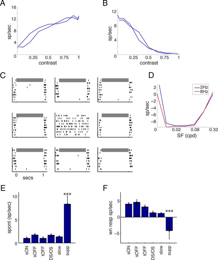
Suppressed by contrast responses. A, Typical response to periodic contrast modulation in the noise movie, showing low baseline response at 0 contrast, up to high firing at full contrast. The double line represents the response as the movie contrast increases up to full contrast and then back down to gray. B, Typical response of a unit in the “suppressed” group shows the opposite response, firing at a high rate in the presence of a uniform gray field, and then strongly suppressed firing to a high contrast scene. C, Spike rasters for unit in B, in response to drifting sinusoidal gratings of a range of orientations, demonstrating near-complete suppression during the grating presentation. Spontaneous firing to an interleaved uniform background is shown in the center. D, Spatial frequency tuning curve of grating-evoked response for unit in B, demonstrating strong suppression for spatial and temporal frequencies that drive most LGN units. E, Median spontaneous firing rate across all groups, showing greatly increased spontaneous rate among the suppressed group. F, Median evoked firing rate during the high-contrast phase of contrast-modulated noise movies, showing sharp reduction in firing in suppressed units. ***p < 0.001.

Furthermore, this suppression of firing occurs across a large range of stimuli that drive the rest of the population. As shown in Figure 6C, during the presentation of a drifting grating of any orientation, the firing of this cell nearly stops. In addition, the spatial frequency tuning curve in Figure 6D shows that from 0.01 to 0.16 cpd, the neuron's firing is strongly reduced relative to spontaneous rate. The only spatial frequencies that do not suppress firing are 0.32 cpd, at the high end of the spatial acuity, and 0 cpd, a full-field flicker that does not contain spatial contrast.

Figure 6E, F compares these properties with the rest of the population. This confirms that suppressed neurons as a population have a dramatically higher baseline firing rate than the rest of the population (Fig. 6E), and are unique in having substantial decreases in firing rate during noise movies (Fig. 6F). Indeed, this decrease is approximately the same magnitude as the increase of firing rate seen in the standard population of center-surround units.

Functional organization of topography and response types

Although the mouse LGN does not have the overt cellular lamination found in other species, classic studies in rat (Martin, 1986; Reese, 1988) suggested that “hidden” segregation of functional pathways is indeed present in the LGN. More recently, genetic methods that label the axonal projections of specific RGC types showed that RGCs with distinct response properties project to different subregions of the LGN (e.g., Off-α RGCs with transient light responses project to the medial portion of the LGN) (Huberman et al., 2008), whereas ON/OFF DS ganglion cells (DSGCs) project to a specific laminar termination zone adjacent to the optic tract (Huberman et al., 2009; Kay et al., 2011; Rivlin-Etzion et al., 2011). Furthermore, a recent morphological study of mouse LGN neurons found three categories of cells that resemble the X, Y, and W LGN neuron morphologies described in the cat; each LGN cell type had distinct, although partially overlapping, distribution in the LGN; most notably, the W-like cells were biased to reside in the region adjacent to the optic tract (Krahe et al., 2011), the same location where the axons of On-Off DS RGCs terminate (Huberman et al., 2009; Rivlin-Etzion et al., 2011).

To assay the functional organization of the LGN, we used the location of each recorded unit (Fig. 1B) to construct functional maps, by combining the sites from individual recordings onto a common LGN template. We used the normalized position within each individual reconstructed LGN, so that even if the shape of the LGN varied slightly from specimen to specimen, the relative location (anterior–posterior, dorsal–ventral, medial–lateral) would be preserved in the ensemble dataset. Furthermore, to account for variations in the density of sampling, we used a spatial interpolation and normalization to calculate smooth maps of functional properties.

In mouse, the 2D map of the visual field in the retina is superimposed onto a 3D structure in the LGN. This is in contrast to other species, such as cats and macaque monkeys, which have distinct cytoarchitectural laminae in the LGN. In those species, each layer contains a separate 2D map of retinotopic space. Given the 3D structure of the mouse LGN, it is not clear how other forms of functional organization would relate to retinotopy. Although anatomical studies have measured the retinotopic organization of RGC axons in the mouse LGN (Pfeiffenberger et al., 2005), no functional analysis of the complete representation of visual space in the mouse LGN has been carried out. By using the RF locations calculated from STA responses to band-limited and sparse noise movies, we constructed retinotopic maps for azimuth and elevation through the LGN, which we present as three A/P sections: anterior, middle, and posterior. As seen in Figure 7A, B, both azimuth and elevation are represented smoothly across the LGN, in approximately orthogonal alignment. There is a mostly complete map of visual space present in each A/P section, although the representation shifts slightly downward in visual space toward the posterior LGN. Thus, because each point in visual space is represented at multiple points throughout the LGN, there is potential for multiple representations to be spatially segregated or have regional biases, perhaps according to specific encoding properties and not unlike other species.

Figure 7.

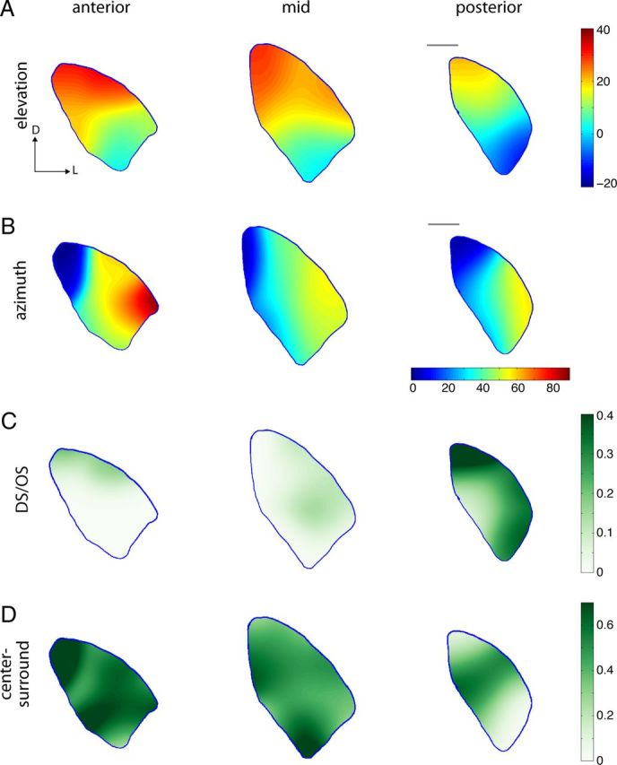
Spatial organization of LGN functional responses. A, B, Interpolated map of RF locations, measured from noise and flashing spot movies, for elevation (A) and azimuth (B), illustrating a smooth progression from dorsomedial to ventrolateral for elevation, and from medial to lateral for azimuth (n = 182 units). D/L, Dorsal/lateral. C, Interpolated map for density of DS/OS units, showing increased prevalence in the posterior LGN and a bias along the dorsolateral edge (n = 257 total units, 28 DS/OS). D, Interpolated map for density of center-surround units (sON, sOFF, tOFF), showing a bias for anterior regions (n = 257 total units, 134 center-surround). Scale bar: A–D, 200 μm. C, D, Color bar represents the proportion of cells of a given type.

To test this, we mapped the location of the different functional groups described above into density maps on the LGN. The most obvious and striking organization was seen for the DS/OS group (Fig. 7C), which was heavily over-represented in the posterior LGN; and throughout the LGN, DS/OS neurons were more likely to be found in the region adjacent to the overlying optic tract. Indeed, this DS/OS-enriched region can be envisioned as wrapping around the dorsolateral surface of the LGN and onto the posterior pole and thus represents a functionally segregated compartment of the mouse LGN. Other cell types showed a less pronounced bias, although the center-surround cell types had a higher density in the anterior LGN, complementing the enrichment of DS/OS in the posterior LGN (Fig. 7D). However, it is clear that there is not a strict segregation, as even at its highest the density of DS/OS cells is ∼40%, and there are always intermingled cells of other types. Indeed, it is important to note that nearby units recorded at the same or at neighboring sites often had different response types.

Comparison with domains of DS tuned retinal inputs and molecular markers of monkey magnocellular and parvocellular channels

Next, we considered the distributions of LGN response properties relative to genetic and molecular markers of different types of incoming RGC afferents and LGN cell types. Our evidence for variations in DS/OS responses along the medial–lateral as well as anterior–posterior extent of the LGN (Fig. 7C, top) prompted us to analyze the axon termination zones arising from On-Off direction-tuned RGCs as a function of their anterior–posterior location, a feature that has not been analyzed or reported previously for any DSGC type. Serial sections through the entire LGN of 8 adult mice were analyzed. The boundaries of the LGN were defined by cytoarchitecture (Fig. 8A–C) and retinogeniculate terminations of all RGCs labeled by intraocular injections of the anterograde tracer cholera toxin β conjugated to Alexa-594 (Fig. 8D,E). By analyzing transgenic mice that selectively express GFP in posterior tuned DS RGCs we observed that axons from these RGCs terminate in the lateral LGN, close to the optic tract (Fig. 8G–I) (Huberman et al., 2009; Rivlin-Etzion et al., 2011; Wei and Feller, 2011). Interestingly, comparison across the anterior–posterior extent of the LGN revealed a systematic expansion of DS terminations as we progressed toward the posterior pole of the LGN. Indeed, within the posterior LGN, DS RGCs terminated across a far greater extent of the LGN (∼60%) compared with within the anterior LGN (∼20%). These observed anterior–posterior variations are nicely aligned with the electrophysiological signatures of DS/OS LGN neurons described above and raise the possibility that the responses of DS/OS LGN neurons are the direct consequence of inputs from direction tuned retinal afferents.

Previous work addressed the question of whether there are histochemical markers of functionally distinct layers and/or cell types in the monkey and cat LGN, prompting us to ask whether the same markers delineate anatomical and/or functional subdivisions of the mouse LGN explored in our study. Chondroitin sulfate proteoglycans are reported as specific to the magnocellular layers of the monkey LGN and the “Y” (sometimes called “A”) layers of the cat LGN (Murray et al., 2008). Also, the transcription factor FoxP2 is specific to the parvocellular layers of the marmoset (Mashiko et al., 2012) and macaque LGN and X cells in carnivores (Iwai et al., 2012). We stained the mouse LGN for these markers and found that, whereas many LGN cells expressed CSPG and Foxp2 (Fig. 8J,K), neither marker displayed any obvious laminar or overt regional biases. It is interesting to note, however, that not every LGN cell expressed CSPG or Foxp2 (Fig. 8L–Q). Thus, if these markers represent Y/magnocellular-like cells or X/parvocellular-like cells, both cell types are scattered in “salt and pepper” fashion throughout the LGN in mouse.

Taken with our analysis of the spatial distributions of LGN neuron response properties, these molecular genetic expression studies underscore the degree to which mouse DS/OS-tuned LGN neurons are strongly localized to a defined area of the LGN, as opposed to the more widespread interspersed distribution of neurons with center-surround and other response properties. To some extent, this latter feature is reminiscent of mouse visual cortex, where orientation selectivity exists at the single-cell level despite the absence of more macroscopic maps, such as orientation pinwheels or columns (Ohki and Reid, 2007).

Discussion

Our recordings and anatomical reconstructions reveal a much higher degree of functional sophistication and compartmentalization in the mouse LGN than previously suspected. Not only does the mouse LGN encode three “standard” types of center-surround RFs, it also encodes two properties not generally thought to be present in the LGN, but that are present in the cortex: orientation selectivity and direction selectivity. The mouse LGN also encodes a suppressed-by-contrast mechanism that signals uniformity of the visual field, and a heterogeneous assembly of slow W-like cells that likely yield even more diversity. Furthermore, the mouse LGN displays a previously unknown aspect of functional organization, with direction and OS units greatly enriched in the posterior and dorsolateral LGN. Importantly, our findings provide a genetically tractable system to investigate the mechanisms of these multiple channels, including both canonical and noncanonical cell types, in cortical computations.

Recording and cluster analysis reveal specific response types

The use of multisite silicon electrodes had multiple advantages for our study. First, we could place them in the LGN and record any neurons present, so we were not limited to recording from cells that were readily activated. Furthermore, we could maintain recordings from an ensemble of neurons over an extended period, allowing us to present an extensive stimulus set necessary to characterize diverse cell types. The linear geometry of the probe enabled us to sample neurons throughout the volume of the LGN, and importantly, to use post hoc histology to determine the spatial location of individual recording sites.

To seek order in the rich array of response types we found from our battery of visual stimuli, we used a clustering algorithm to generate groups with related response profiles, as has been performed previously for RGCs (Carcieri et al., 2003; Farrow and Masland, 2011). This yielded six broad groups that could be approximately mapped onto previously described retinal or LGN cell types. This approach thereby allowed us to extract groups of neurons with similar response profiles, without relying on fixed thresholds, such as the standard 3:1 selectivity for orientation tuning. Clustering allows the entire response profile to be used and, in our case, found patterns of response properties that varied together within groups. It also allows the discovery of distinctions that may not have been expected a priori. However, because the choice of number of clusters to generate was made for classification purposes, it is not to be taken as a rigorous definition of the total number of distinct channels in the LGN.

It is not clear why the diverse cell types we delineate have not been widely described in the LGN of other species, despite the fact that there are scattered examples of each unusual type described in the literature (for review, see Masland and Martin, 2007). It may be that standard stimulus sets do not probe for these response types, or they may get classified as unresponsive or outliers. Furthermore, it appears they make up a higher proportion of the total LGN neuron population in mouse than other species where they have been reported. Species with high acuity may need a far greater number of center-surround units to cover the visual field; if the absolute number of noncanonical neurons needed to span the same area does not change across species, this could explain the lower density.

Direction and orientation selectivity along the retino-geniculo-V1 pathway

The presence of direction and orientation selectivity in the LGN, although not entirely unprecedented (Levick et al., 1969; Thompson et al., 1994), raises important questions about both the source of their tuning and their role in defining RFs properties in cortex. Direction-tuned RGCs were first described in the retinas of rabbits (Barlow and Hill, 1963) and more recently were characterized in the mouse retina (Weng et al., 2005; Huberman et al., 2009; Kay et al., 2011; Rivlin-Etzion et al., 2011). A recent in vivo imaging study of mouse LGN also confirmed the existence of DS/OS (Marshel et al., 2012), although they reported primarily anterior–posterior selectivity, rather than all four cardinal directions of selectivity as observed here. The discrepancy in findings may be because their imaging was restricted to the superficial-most 75 μm of the LGN, whereas the penetrating electrode recordings we describe here could survey all portions of the LGN and thus identify a greater number and diversity of cell types.

It is interesting to note that, although we found DS/OS cells strongly tuned for each cardinal axis of motion (up, down, left, and right), there were few DS/OS cells with peak tuning for intermediate directions (e.g., 45°). The DSGCs that project to the LGN also display this cardinal-biased tuning. Furthermore, the spatiotemporal properties of these units, including ON/OFF responses and tuning for low speeds, are consistent with DSGCs in the retina (Weng et al., 2005). Combined with the fact that DS/OS LGN neurons lie in direct register with DSGC axon terminations along the full anterior–posterior extent of the LGN (Figs. 7 and 8), our data suggest that many DS/OS LGN neurons may derive their motion selectivity directly from RGC tuning.

It is particularly striking that OS responses were much more abundant than DS responses in the LGN because a number of DS RGCs have been identified, but so far reports of OS responses in the retina are scarce. Given that mature LGN neurons receive input from three or fewer RGCs (Chen and Regehr, 2000; Jaubert-Miazza et al., 2005), our findings are consistent with the possibility that OS tuning of mouse LGN neurons arises from combined influences of two or three DS tuned RGCs, as in a recently proposed model based on in vivo imaging (Marshel et al., 2012). This would be a novel method of computing orientation/axial selectivity, in contrast to the classic model of OS tuning for V1 neurons arising from a linear array of center-surround RFs (Hubel and Wiesel, 1962). It also raises the striking developmental question of how LGN neurons could specifically restrict input to two opposed directions of motion, rather than pooling other directions as well.

Does the cortex inherit direction and/or orientation selectivity from the LGN, or is it computed anew? It appears unlikely that the orientation selectivity seen in mouse LGN is directly inherited, as mouse V1 OS units are primarily simple/linear cells, whereas the DS/OS units we found in LGN were generally nonlinear. Furthermore, the DS/OS population is a still a small fraction of the LGN population, relative to the population of center-surround neurons that could support OS by traditional summation models (Hubel and Wiesel, 1962; Chapman et al., 1991; Alonso et al., 2001). However, it is possible that the selectivity transmitted from the LGN could provide a scaffold for developmental processes that shape DS/OS in V1 (Rochefort et al., 2011). It is also possible that the DS/OS cells from LGN provide a dedicated channel to a subset of nonlinear neurons in V1. In either case, our results suggest the need to extend models of circuitry in the cortex of the mouse to include directionally tuned input from the LGN.

Suppressed by contrast: an unknown role in visual processing

The “suppressed” group clearly corresponds to suppressed-by-contrast units, a type of rarely encountered neuron that has been described in the retina of cat (Rodieck, 1967) and rabbit (Levick, 1967), as well as the monkey LGN (Tailby et al., 2007). These responses have also been found in V1 of awake mice (Niell and Stryker, 2010), where they are strongly modulated by behavioral state: when an animal is stationary, the cells are inactive; but when the animal initiates locomotion, the cells greatly increase their firing rate and show the suppression to a broad range of contrast stimuli described here.

The role of suppressed-by-contrast neurons is an open question because they run counter to most ideas of visual processing and have only been described in a few studies. However, the results presented here and previously (Niell and Stryker, 2010) demonstrate that their numbers are not insignificant in the mouse visual system. It has been proposed that they could provide a signal to control contrast gain (Troy et al., 1989) or serve to mask out regions of constant illumination (Masland and Martin, 2007). It is also possible, particularly given their “inverse” response relative to the rest of the population, that these cells are inhibitory interneurons, although their presence in the retina and cortex as well suggests a projection pathway.

Possible homology of other types

The center-surround units we found resemble the standard pathways described in other species (Nassi and Callaway, 2009), parvocellular and magnocellular in primates and X and Y in carnivores. Because the homology between these two pathways in primates versus carnivores is still not clear, it is difficult to map our response types directly onto the two pathways. We do find a distinction between sustained and transient responses, which often distinguishes parvocellular/magnocellular and X/Y. However, similar to the results of Grubb and Thompson (2003), we do not find other striking differences between the sustained and transient cells, such as RF size or linearity. Strikingly, the three types we found do correspond closely to physiological properties of mouse α RGCs, including the absence of an On-transient type (Pang et al., 2003; van Wyk et al., 2009). This suggests that α RGCs provide the primary input to the canonical pathways; however, this remains to be tested, and indeed the lack of On-transient responses could extend to other retinal populations as well.

Furthermore, although we found some spatial correspondence between DS/OS neurons and cells morphologically described as “W” cells (Krahe et al., 2011), we did not see a clear spatial segregation of our center-surround units corresponding to Krahe et al.'s described morphological X/Y distributions, either in functional maps or anatomical markers that label these cell types in carnivores and primates. Together, these results suggest that we may not have found the appropriate distinction that correlates with these morphologies, or that different mapping methods are needed to detect their differences in distributions, if those differences exist. One imagines that the homology of mouse versus primate and cat LGN neurons may be clarified, in part, by studies of the cortical areas and cortical layers these functionally and anatomically defined LGN neuron types project to and/or receive feedback from (Briggs and Usrey, 2009; Nassi and Callaway, 2009).

It is of interest that the third classically described visual pathway through the primate LGN, termed koniocellular (or “W” in cats), generally shows less brisk visually evoked activity and a fairly broad range of tuning properties (Casagrande, 1994; Hendry and Reid, 2000). The “slow” group we found bears many similarities to this pathway, including long latencies and response to both ON and OFF. To date, attempts to classify the range of koniocellular/W responses have been limited, primarily because of their diversity; however, the relative abundance and potential for genetic access in mice may lead to more insight. Furthermore, experiments tailored to identify other noncanonical RGC types, such as local edge detectors (Zeck et al., 2005; Russell and Werblin, 2010), may find them in this diverse group, or within the small fraction of units that were not responsive to our stimulus set.

Convergence and relative numbers of RGC versus LGN neurons with similar response properties

It is worth noting that the relative proportion of center-surround and DS/OS neurons in mouse LGN is almost opposite the proportion of their counterparts in the retina. On and Off α RGCs represent ∼5% of the total RGC population in mouse (Pang et al., 2003; Huberman et al., 2008), and yet the percentages of LGN neurons recorded with sON, sOFF, or tOFF responses was at least double that value for each type. This could be because α RGCs preferentially target the LGN, relative to other RGC subtypes in the mouse; and indeed, there is evidence for this (e.g., compare Huberman et al., 2008; Osterhout et al., 2011). A nonmutually exclusive possibility is that, because mouse α RGC axonal arbors are relatively large (Pang et al., 2003; Huberman et al., 2008; Hong et al., 2011; and A.D. Huberman, unpublished observations), they may innvervate far more LGN neurons than their absolute numbers suggest.

There is a mismatch in the opposite direction for the relative number of On-Off DS RGCs versus LGN neurons with DS/OS properties. Assuming approximately equal numbers of each subtype representing each of the four cardinal axes, On-Off DSGCs comprise ∼40–50% of the RGCs in the mouse (Huberman et al., 2009; Kay et al., 2011; Rivlin-Etzion et al., 2011), whereas the overall number of DS/OS LGN neurons is about one-fourth that value. In contrast to α RGCs, On-Off DSGCs restrict their axons to a narrow region of the LGN (Fig. 8), which can partly explain this relative mismatch.

In conclusion, together, our data reveal the rich repertoire of visual signals contained in the mouse LGN and, therefore, that are conveyed to visual cortex. Given that many of the RGC types that generate this information have been genetically identified in the mouse, it should soon be possible to causally assess the impact of specific retinal output pathways on LGN and cortical processing, using cell-type-specific manipulations of activity (Zhang et al., 2007; Alexander et al., 2009). In the future, genetic identification and manipulation of specific LGN neuron types should also be immensely useful for understanding how visual information is encoded and transformed in the geniculocortical pathways, and their role in driving specific aspects of perception and behavior.

References

- Alexander GM, Rogan SC, Abbas AI, Armbruster BN, Pei Y, Allen JA, Nonneman RJ, Hartmann J, Moy SS, Nicolelis MA, McNamara JO, Roth BL. Remote control of neuronal activity in transgenic mice expressing evolved G protein-coupled receptors. Neuron. 2009;63:27–39. doi: 10.1016/j.neuron.2009.06.014. [DOI] [PMC free article] [PubMed] [Google Scholar]
- Alonso JM, Usrey WM, Reid RC. Rules of connectivity between geniculate cells and simple cells in cat primary visual cortex. J Neurosci. 2001;21:4002–4015. doi: 10.1523/JNEUROSCI.21-11-04002.2001. [DOI] [PMC free article] [PubMed] [Google Scholar]
- Andermann ML, Kerlin AM, Roumis DK, Glickfeld LL, Reid RC. Functional specialization of mouse higher visual cortical areas. Neuron. 2011;72:1025–1039. doi: 10.1016/j.neuron.2011.11.013. [DOI] [PMC free article] [PubMed] [Google Scholar]
- Atallah BV, Bruns W, Carandini M, Scanziani M. Parvalbumin-expressing interneurons linearly transform cortical responses to visual stimuli. Neuron. 2012;73:159–170. doi: 10.1016/j.neuron.2011.12.013. [DOI] [PMC free article] [PubMed] [Google Scholar]
- Barlow HB, Hill RM. Selective sensitivity to direction of movement in ganglion cells of the rabbit retina. Science. 1963;139:412–414. doi: 10.1126/science.139.3553.412. [DOI] [PubMed] [Google Scholar]
- Bonin V, Histed MH, Yurgenson S, Reid RC. Local diversity and fine-scale organization of receptive fields in mouse visual cortex. J Neurosci. 2011;31:18506–18521. doi: 10.1523/JNEUROSCI.2974-11.2011. [DOI] [PMC free article] [PubMed] [Google Scholar]
- Brainard DH. The Psychophysics Toolbox. Spatial Vision. 1997;10:433–436. [PubMed] [Google Scholar]
- Briggs F, Usrey WM. Parallel processing in the corticogeniculate pathway of the macaque monkey. Neuron. 2009;62:135–146. doi: 10.1016/j.neuron.2009.02.024. [DOI] [PMC free article] [PubMed] [Google Scholar]
- Cang J, Niell CM, Liu X, Pfeiffenberger C, Feldheim DA, Stryker MP. Selective disruption of one Cartesian axis of cortical maps and receptive fields by deficiency in ephrin-As and structured activity. Neuron. 2008;57:511–523. doi: 10.1016/j.neuron.2007.12.025. [DOI] [PMC free article] [PubMed] [Google Scholar]
- Carcieri SM, Jacobs AL, Nirenberg S. Classification of retinal ganglion cells: a statistical approach. J Neurophysiol. 2003;90:1704–1713. doi: 10.1152/jn.00127.2003. [DOI] [PubMed] [Google Scholar]
- Casagrande VA. A third parallel visual pathway to primate area V1. Trends Neurosci. 1994;17:305–310. doi: 10.1016/0166-2236(94)90065-5. [DOI] [PubMed] [Google Scholar]
- Chapman B, Zahs KR, Stryker MP. Relation of cortical cell orientation selectivity to alignment of receptive fields of the geniculocortical afferents that arborize within a single orientation column in ferret visual cortex. J Neurosci. 1991;11:1347–1358. doi: 10.1523/JNEUROSCI.11-05-01347.1991. [DOI] [PMC free article] [PubMed] [Google Scholar]
- Chen C, Regehr WG. Developmental remodeling of the retinogeniculate synapse. Neuron. 2000;28:955–966. doi: 10.1016/s0896-6273(00)00166-5. [DOI] [PubMed] [Google Scholar]
- Dacey DM, Peterson BB, Robinson FR, Gamlin PD. Fireworks in the primate retina: in vitro photodynamics reveals diverse LGN-projecting ganglion cell types. Neuron. 2003;37:15–27. doi: 10.1016/s0896-6273(02)01143-1. [DOI] [PubMed] [Google Scholar]
- Farrow K, Masland RH. Physiological clustering of visual channels in the mouse retina. J Neurophysiol. 2011;105:1516–1530. doi: 10.1152/jn.00331.2010. [DOI] [PMC free article] [PubMed] [Google Scholar]
- Field GD, Chichilnisky EJ. Information processing in the primate retina: circuitry and coding. Annu Rev Neurosci. 2007;30:1–30. doi: 10.1146/annurev.neuro.30.051606.094252. [DOI] [PubMed] [Google Scholar]
- Gao E, DeAngelis GC, Burkhalter A. Parallel input channels to mouse primary visual cortex. J Neurosci. 2010;30:5912–5926. doi: 10.1523/JNEUROSCI.6456-09.2010. [DOI] [PMC free article] [PubMed] [Google Scholar]
- Gollisch T, Meister M. Eye smarter than scientists believed: neural computations in circuits of the retina. Neuron. 2010;65:150–164. doi: 10.1016/j.neuron.2009.12.009. [DOI] [PMC free article] [PubMed] [Google Scholar]
- Grubb MS, Thompson ID. Quantitative characterization of visual response properties in the mouse dorsal lateral geniculate nucleus. J Neurophysiol. 2003;90:3594–3607. doi: 10.1152/jn.00699.2003. [DOI] [PubMed] [Google Scholar]
- Harris KD, Henze DA, Csicsvari J, Hirase H, Buzsáki G. Accuracy of tetrode spike separation as determined by simultaneous intracellular and extracellular measurements. J Neurophysiol. 2000;84:401–414. doi: 10.1152/jn.2000.84.1.401. [DOI] [PubMed] [Google Scholar]
- Hendry SH, Reid RC. The koniocellular pathway in primate vision. Annu Rev Neurosci. 2000;23:127–153. doi: 10.1146/annurev.neuro.23.1.127. [DOI] [PubMed] [Google Scholar]
- Hirsch JA, Martinez LM. Circuits that build visual cortical receptive fields. Trends Neurosci. 2006;29:30–39. doi: 10.1016/j.tins.2005.11.001. [DOI] [PubMed] [Google Scholar]
- Hong YK, Kim IJ, Sanes JR. Stereotyped axonal arbors of retinal ganglion cell subsets in the mouse superior colliculus. J Comp Neurol. 2011;519:1691–1711. doi: 10.1002/cne.22595. [DOI] [PMC free article] [PubMed] [Google Scholar]
- Hubel DH, Wiesel TN. Receptive fields, binocular interaction and functional architecture in the cat's visual cortex. J Physiol. 1962;160:106–154. doi: 10.1113/jphysiol.1962.sp006837. [DOI] [PMC free article] [PubMed] [Google Scholar]
- Hübener M. Mouse visual cortex. Curr Opin Neurobiol. 2003;13:413–420. doi: 10.1016/s0959-4388(03)00102-8. [DOI] [PubMed] [Google Scholar]
- Huberman AD, Niell CM. What can mice tell us about how vision works? Trends Neurosci. 2011;34:464–473. doi: 10.1016/j.tins.2011.07.002. [DOI] [PMC free article] [PubMed] [Google Scholar]
- Huberman AD, Manu M, Koch SM, Susman MW, Lutz AB, Ullian EM, Baccus SA, Barres BA. Architecture and activity-mediated refinement of axonal projections from a mosaic of genetically identified retinal ganglion cells. Neuron. 2008;59:425–438. doi: 10.1016/j.neuron.2008.07.018. [DOI] [PMC free article] [PubMed] [Google Scholar]
- Huberman AD, Wei W, Elstrott J, Stafford BK, Feller MB, Barres BA. Genetic identification of an On-Off direction-selective retinal ganglion cell subtype reveals a layer-specific subcortical map of posterior motion. Neuron. 2009;62:327–334. doi: 10.1016/j.neuron.2009.04.014. [DOI] [PMC free article] [PubMed] [Google Scholar]
- Iwai L, Ohashi Y, van der List D, Usrey WM, Miyashita Y, Kawasaki H. FoxP2 is a parvocellular-specific transcription factor in the visual thalamus of monkeys and ferrets. Cereb Cortex. 2012 doi: 10.1093/cercor/bhs207. Advance online publication. Retrieved July 12, 2012. [DOI] [PMC free article] [PubMed] [Google Scholar]
- Jaubert-Miazza L, Green E, Lo FS, Bui K, Mills J, Guido W. Structural and functional composition of the developing retinogeniculate pathway in the mouse. Vis Neurosci. 2005;22:661–676. doi: 10.1017/S0952523805225154. [DOI] [PubMed] [Google Scholar]
- Kaneko M, Hanover JL, England PM, Stryker MP. TrkB kinase is required for recovery, but not loss, of cortical responses following monocular deprivation. Nat Neurosci. 2008;11:497–504. doi: 10.1038/nn2068. [DOI] [PMC free article] [PubMed] [Google Scholar]
- Kay JN, De la Huerta I, Kim IJ, Zhang Y, Yamagata M, Chu MW, Meister M, Sanes JR. Retinal ganglion cells with distinct directional preferences differ in molecular identity, structure, and central projections. J Neurosci. 2011;31:7753–7762. doi: 10.1523/JNEUROSCI.0907-11.2011. [DOI] [PMC free article] [PubMed] [Google Scholar]
- Kerlin AM, Andermann ML, Berezovskii VK, Reid RC. Broadly tuned response properties of diverse inhibitory neuron subtypes in mouse visual cortex. Neuron. 2010;67:858–871. doi: 10.1016/j.neuron.2010.08.002. [DOI] [PMC free article] [PubMed] [Google Scholar]
- Krahe TE, El-Danaf RN, Dilger EK, Henderson SC, Guido W. Morphologically distinct classes of relay cells exhibit regional preferences in the dorsal lateral geniculate nucleus of the mouse. J Neurosci. 2011;31:17437–17448. doi: 10.1523/JNEUROSCI.4370-11.2011. [DOI] [PMC free article] [PubMed] [Google Scholar]
- Lee SH, Kwan AC, Zhang S, Phoumthipphavong V, Flannery JG, Masmanidis SC, Taniguchi H, Huang ZJ, Zhang F, Boyden ES, Deisseroth K, Dan Y. Activation of specific interneurons improves V1 feature selectivity and visual perception. Nature. 2012;488:379–383. doi: 10.1038/nature11312. [DOI] [PMC free article] [PubMed] [Google Scholar]
- Levick WR. Receptive fields and trigger features of ganglion cells in the visual streak of the rabbits retina. J Physiol. 1967;188:285–307. doi: 10.1113/jphysiol.1967.sp008140. [DOI] [PMC free article] [PubMed] [Google Scholar]
- Levick WR, Oyster CW, Takahashi E. Rabbit lateral geniculate nucleus: sharpener of directional information. Science. 1969;165:712–714. doi: 10.1126/science.165.3894.712. [DOI] [PubMed] [Google Scholar]
- Liu BH, Li YT, Ma WP, Pan CJ, Zhang LI, Tao HW. Broad inhibition sharpens orientation selectivity by expanding input dynamic range in mouse simple cells. Neuron. 2011;71:542–554. doi: 10.1016/j.neuron.2011.06.017. [DOI] [PMC free article] [PubMed] [Google Scholar]
- Marr D, Ullman S. Directional selectivity and its use in early visual processing. Proc R Soc Lond B Biol Sci. 1981;211:151–180. doi: 10.1098/rspb.1981.0001. [DOI] [PubMed] [Google Scholar]
- Marshel JH, Kaye AP, Nauhaus I, Callaway EM. Anterior–posterior direction opponency in the superficial mouse lateral geniculate nucleus. Neuron. 2012;76:713–720. doi: 10.1016/j.neuron.2012.09.021. [DOI] [PMC free article] [PubMed] [Google Scholar]
- Martin PR. The projection of different retinal ganglion cell classes to the dorsal lateral geniculate nucleus in the hooded rat. Exp Brain Res. 1986;62:77–88. doi: 10.1007/BF00237404. [DOI] [PubMed] [Google Scholar]
- Mashiko H, Yoshida AC, Kikuchi SS, Niimi K, Takahashi E, Aruga J, Okano H, Shimogori T. Comparative anatomy of marmoset and mouse cortex from genomic expression. J Neurosci. 2012;32:5039–5053. doi: 10.1523/JNEUROSCI.4788-11.2012. [DOI] [PMC free article] [PubMed] [Google Scholar]
- Masland RH, Martin PR. The unsolved mystery of vision. Curr Biol. 2007;17:R577–R582. doi: 10.1016/j.cub.2007.05.040. [DOI] [PubMed] [Google Scholar]
- McLean J, Raab S, Palmer LA. Contribution of linear mechanisms to the specification of local motion by simple cells in areas 17 and 18 of the cat. Vis Neurosci. 1994;11:271–294. doi: 10.1017/s0952523800001632. [DOI] [PubMed] [Google Scholar]
- Murray KD, Rubin CM, Jones EG, Chalupa LM. Molecular correlates of laminar differences in the macaque dorsal lateral geniculate nucleus. J Neurosci. 2008;28:12010–12022. doi: 10.1523/JNEUROSCI.3800-08.2008. [DOI] [PMC free article] [PubMed] [Google Scholar]
- Nassi JJ, Callaway EM. Parallel processing strategies of the primate visual system. Nat Rev Neurosci. 2009;10:360–372. doi: 10.1038/nrn2619. [DOI] [PMC free article] [PubMed] [Google Scholar]
- Niell CM, Stryker MP. Highly selective receptive fields in mouse visual cortex. J Neurosci. 2008;28:7520–7536. doi: 10.1523/JNEUROSCI.0623-08.2008. [DOI] [PMC free article] [PubMed] [Google Scholar]
- Niell CM, Stryker MP. Modulation of visual responses by behavioral state in mouse visual cortex. Neuron. 2010;65:472–479. doi: 10.1016/j.neuron.2010.01.033. [DOI] [PMC free article] [PubMed] [Google Scholar]
- Ohki K, Reid RC. Specificity and randomness in the visual cortex. Curr Opin Neurobiol. 2007;17:401–407. doi: 10.1016/j.conb.2007.07.007. [DOI] [PMC free article] [PubMed] [Google Scholar]
- Olsen SR, Bortone DS, Adesnik H, Scanziani M. Gain control by layer six in cortical circuits of vision. Nature. 2012;483:47–52. doi: 10.1038/nature10835. [DOI] [PMC free article] [PubMed] [Google Scholar]
- Osterhout JA, Josten N, Yamada J, Pan F, Wu SW, Nguyen PL, Panagiotakos G, Inoue YU, Egusa SF, Volgyi B, Inoue T, Bloomfield SA, Barres BA, Berson DM, Feldheim DA, Huberman AD. Cadherin-6 mediates axon-target matching in a non-image-forming visual circuit. Neuron. 2011;71:632–639. doi: 10.1016/j.neuron.2011.07.006. [DOI] [PMC free article] [PubMed] [Google Scholar]
- Pang JJ, Gao F, Wu SM. Light-evoked excitatory and inhibitory synaptic inputs to ON and OFF α ganglion cells in the mouse retina. J Neurosci. 2003;23:6063–6073. doi: 10.1523/JNEUROSCI.23-14-06063.2003. [DOI] [PMC free article] [PubMed] [Google Scholar]
- Pelli DG. The VideoToolbox software for visual psychophysics: transforming numbers into movies. Spat Vis. 1997;10:437–442. [PubMed] [Google Scholar]
- Pfeiffenberger C, Cutforth T, Woods G, Yamada J, Rentería RC, Copenhagen DR, Flanagan JG, Feldheim DA. Ephrin-As and neural activity are required for eye-specific patterning during retinogeniculate mapping. Nat Neurosci. 2005;8:1022–1027. doi: 10.1038/nn1508. [DOI] [PMC free article] [PubMed] [Google Scholar]
- Reese BE. ‘Hidden lamination’ in the dorsal lateral geniculate nucleus: the functional organization of this thalamic region in the rat. Brain Res. 1988;472:119–137. doi: 10.1016/0165-0173(88)90017-3. [DOI] [PubMed] [Google Scholar]
- Ringach DL. Spatial structure and symmetry of simple-cell receptive fields in macaque primary visual cortex. J Neurophysiol. 2002;88:455–463. doi: 10.1152/jn.2002.88.1.455. [DOI] [PubMed] [Google Scholar]
- Ringach DL, Shapley RM, Hawken MJ. Orientation selectivity in macaque V1: diversity and laminar dependence. J Neurosci. 2002;22:5639–5651. doi: 10.1523/JNEUROSCI.22-13-05639.2002. [DOI] [PMC free article] [PubMed] [Google Scholar]
- Rivlin-Etzion M, Zhou K, Wei W, Elstrott J, Nguyen PL, Barres BA, Huberman AD, Feller MB. Transgenic mice reveal unexpected diversity of on-off direction-selective retinal ganglion cell subtypes and brain structures involved in motion processing. J Neurosci. 2011;31:8760–8769. doi: 10.1523/JNEUROSCI.0564-11.2011. [DOI] [PMC free article] [PubMed] [Google Scholar]
- Rochefort NL, Narushima M, Grienberger C, Marandi N, Hill DN, Konnerth A. Development of direction selectivity in mouse cortical neurons. Neuron. 2011;71:425–432. doi: 10.1016/j.neuron.2011.06.013. [DOI] [PubMed] [Google Scholar]
- Rodieck RW. Receptive fields in the cat retina: a new type. Science. 1967;157:90–92. doi: 10.1126/science.157.3784.90. [DOI] [PubMed] [Google Scholar]
- Russell TL, Werblin FS. Retinal synaptic pathways underlying the response of the rabbit local edge detector. J Neurophysiol. 2010;103:2757–2769. doi: 10.1152/jn.00987.2009. [DOI] [PMC free article] [PubMed] [Google Scholar]
- Schmitzer-Torbert N, Jackson J, Henze D, Harris K, Redish AD. Quantitative measures of cluster quality for use in extracellular recordings. Neuroscience. 2005;131:1–11. doi: 10.1016/j.neuroscience.2004.09.066. [DOI] [PubMed] [Google Scholar]
- Sharpee T, Rust NC, Bialek W. Analyzing neural responses to natural signals: maximally informative dimensions. Neural Comput. 2004;16:223–250. doi: 10.1162/089976604322742010. [DOI] [PubMed] [Google Scholar]
- Skottun BC, De Valois RL, Grosof DH, Movshon JA, Albrecht DG, Bonds AB. Classifying simple and complex cells on the basis of response modulation. Vision Res. 1991;31:1079–1086. doi: 10.1016/0042-6989(91)90033-2. [DOI] [PubMed] [Google Scholar]
- Tailby C, Solomon SG, Dhruv NT, Majaj NJ, Sokol SH, Lennie P. A new code for contrast in the primate visual pathway. J Neurosci. 2007;27:3904–3909. doi: 10.1523/JNEUROSCI.5343-06.2007. [DOI] [PMC free article] [PubMed] [Google Scholar]
- Thompson KG, Leventhal AG, Zhou Y, Liu D. Stimulus dependence of orientation and direction sensitivity of cat LGNd relay cells without cortical inputs: a comparison with area 17 cells. Vis Neurosci. 1994;11:939–951. doi: 10.1017/s0952523800003898. [DOI] [PubMed] [Google Scholar]
- Troy JB, Einstein G, Schuurmans RP, Robson JG, Enroth-Cugell C. Responses to sinusoidal gratings of two types of very nonlinear retinal ganglion cells of cat. Vis Neurosci. 1989;3:213–223. doi: 10.1017/s0952523800009974. [DOI] [PubMed] [Google Scholar]
- van Wyk M, Wässle H, Taylor WR. Receptive field properties of ON- and OFF-ganglion cells in the mouse retina. Vis Neurosci. 2009;26:297–308. doi: 10.1017/S0952523809990137. [DOI] [PMC free article] [PubMed] [Google Scholar]
- Weng S, Sun W, He S. Identification of ON-OFF direction-selective ganglion cells in the mouse retina. J Physiol. 2005;562:915–923. doi: 10.1113/jphysiol.2004.076695. [DOI] [PMC free article] [PubMed] [Google Scholar]
- Wei W, Feller MB. Organization and development of direction-selective circuits in the retina. Trends Neurosci. 2011;34:638–645. doi: 10.1016/j.tins.2011.08.002. [DOI] [PMC free article] [PubMed] [Google Scholar]
- Wiesel TN, Hubel DH. Spatial and chromatic interactions in the lateral geniculate body of the rhesus monkey. J Neurophysiol. 1966;29:1115–1156. doi: 10.1152/jn.1966.29.6.1115. [DOI] [PubMed] [Google Scholar]
- Wilson NR, Runyan CA, Wang FL, Sur M. Division and subtraction by distinct cortical inhibitory networks in vivo. Nature. 2012;488:343–348. doi: 10.1038/nature11347. [DOI] [PMC free article] [PubMed] [Google Scholar]
- Wolfe J, Palmer LA. Temporal diversity in the lateral geniculate nucleus of cat. Vis Neurosci. 1998;15:653–675. doi: 10.1017/s0952523898154068. [DOI] [PubMed] [Google Scholar]
- Zeck GM, Xiao Q, Masland RH. The spatial filtering properties of local edge detectors and brisk-sustained retinal ganglion cells. Eur J Neurosci. 2005;22:2016–2026. doi: 10.1111/j.1460-9568.2005.04390.x. [DOI] [PubMed] [Google Scholar]
- Zhang F, Aravanis AM, Adamantidis A, de Lecea L, Deisseroth K. Circuit-breakers: optical technologies for probing neural signals and systems. Nat Rev Neurosci. 2007;8:577–581. doi: 10.1038/nrn2192. [DOI] [PubMed] [Google Scholar]