Estimating Velocity for Processive Motor Proteins with Random Detachment

Abstract

We show that, for a wide range of models, the empirical velocity of processive motor proteins has a limiting Pearson type VII distribution with finite mean but infinite variance. We develop maximum likelihood inference for this Pearson type VII distribution. In two simulation studies, we compare the performance of our MLE with the performance of standard Student’s t-based inference. The studies show that incorrectly assuming normality (1) can lead to imprecise inference regarding motor velocity in the one-sample case, and (2) can significantly reduce power in the two-sample case. These results should be of interest to experimentalists who wish to engineer motors possessing specific functional characteristics.

1. INTRODUCTION

Processive motor proteins are ATP-powered biological nanomachines that drive many forms of movement in living organisms. For example, kinesin and cytoplasmic dynein motors transport payloads, such as organelles or vesicles, through the cytoplasm of eukaryotic cells. The existence of eukaryotic organisms depends on these tiny motors because the passive process of diffusion is not sufficient to transport large and/or massive payloads through the crowded cytoplasm in a timely fashion. This is especially true for transport within neurons, which can be up to a meter in length. A motor protein overcomes these difficulties by hydrolyzing ATP in order to tow a cargo rapidly and in a directed path along a suitable substrate. An understanding of these motors could lead to important biomedical applications, e.g., anti-tumor technologies, treatments for neurodegenerative diseases, devices for blood testing and genetic screening, and treatments for diseases caused by motor protein defects (Hirokawa and Takemura 2003) such as Charcot–Marie–Tooth disease and Usher syndrome.

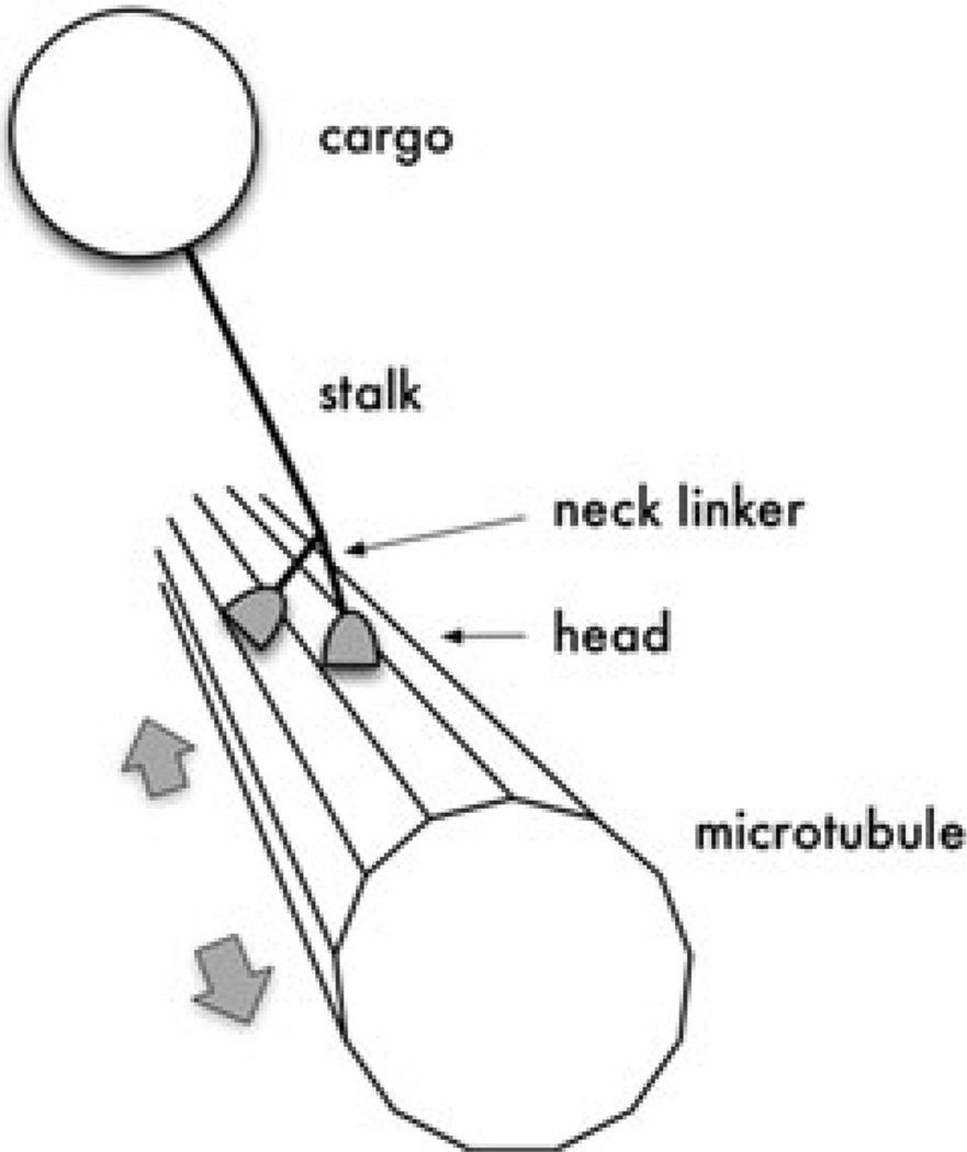
An important type of motor protein is kinesin, of which over 40 varieties have been identified in humans alone (Miki et al. 2001). A conventional kinesin, depicted in Figure 1, comprises two heads, two neck linkers, a coiled-coil stalk, and a tail (Hirokawa et al. 1989; Yang, Laymon, and Goldstein 1989). Each neck linker connects one of the heads to the proximal end of the stalk. At the distal end of the stalk is the tail, which binds the motor’s cargo. The motor “steps” along a microtubule—a type of cylindrical polymer having a regular sequence of binding sites along its surface—with the heads serving as “feet” and the neck linkers serving as “legs.” Eventually the motor dissociates from the microtubule after having taken some random number of steps, typically on the order of a hundred. Each step is governed by a series of chemical reactions along with tethered diffusion, which occurs after the stepping head unbinds from the microtubule and before it rebinds to the microtubule. A step can be either forward or backward, but the motor’s “design” strongly favors forward stepping. For most varieties of kinesin, “forward” means toward the plus end of the microtubule, which is typically oriented toward the cell membrane.

Figure 1.

A kinesin motor protein traversing a microtubule. The figure is not drawn to scale—a kinesin is many times smaller than its cargo. For a typical kinesin, the maximum distance between the heads is approximately 8 nm, whereas a mitochondrion cargo, for example, would have a diameter of 500–10,000 nm.

The above mentioned combination of chemical reactions and diffusion determines both the duration and direction of a step, and also allows for the eventual dissociation of the motor from the microtubule. In the remainder of this article we will refer to the random duration, or dwell time, of the ith step as τ_i (with mean μ_τ and variance ${\sigma }_{\tau }^2$) and the displacement of the ith step (in microtubule binding sites) as Z_i (with mean μ_z and variance ${\sigma }_z^2$). Most models from the motor literature can be adapted to this framework (see reviews by Kolomeisky and Fisher 2007; and Mogilner et al. 2002). For example, standard kinetic models and Brownian models with a spatially periodic structure (such as the model of Elston and Peskin 2000) fit into this framework, as do more detailed stepping models (Atzberger and Peskin 2006; Kutys, Fricks, and Hancock 2010).

Given this coarse description of stepping, and assuming no detachment and an infinitely long microtubule, one can derive the standard quantities of interest for molecular motors, namely, asymptotic velocity and effective diffusion. In fact, a functional central limit theorem (FCLT) can be derived which shows that, in a limiting sense, the moments of step size and duration, along with the covariance between τ_i and Z_i, are all one needs to know (Hughes, Hancock, and Fricks 2011, 2012).

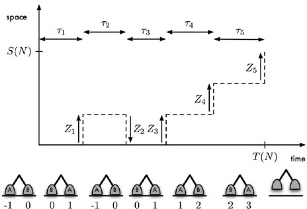
However, as we mentioned above, a motor does not walk indefinitely but rather becomes detached after having taken a large but random number of steps (denoted as N), a fact that has been largely neglected in the modeling literature. In this article we will present results pertaining to this biologically relevant fact. In particular, we focus on the asymptotic behavior of $T(N)={\sum }_{i=1}^N{\tau }_i$ and $S(N)={\sum }_{i=1}^N{Z}_i$, the travel duration and displacement, respectively, as detachment becomes less likely. Figure 2 shows how these quantities can be used to describe processivity.

Figure 2.

A diagrammatic representation of processivity. The motor depicted took five steps (N = 5) before dissociating at time $T(N)={\sum }_{i=1}^{N=5}{\tau }_i$. Steps 1, 3, 4, and 5 were forward steps (Z₁ = Z₃ = Z₄ = Z₅ = 1), and step 2 was backward (Z₂ = −1). Hence the displacement at dissociation was S(N) = 3. The figure below each dwell shows the position of the motor’s two heads at the end of the dwell. The location of the front head at time 0 is taken to be 0.

If we could observe the direction and duration of each motor step, detailed dynamics of the motor could be used to understand the underlying chemical and mechanical structure of a step. However, the experiments typically performed, such as FIONA (Kural, Balci, and Selvin 2005) and laser trap (Spudich et al. 2011) experiments, are often too coarse to allow for such detailed observation. This is why coarsening limits such as functional central limit theorems are important: they allow one to link within-step models to multiple-step models.

For each type of experiment, we do have access to a motor’s total displacement and total travel duration. Using these data, the natural estimator for the velocity of a motor is the ratio of the displacement, S(N), to the total time prior to detachment, T(N):

$$\mathrm{V̂}=\frac{S(N)}{T(N)}=\frac{{\sum }_{i=1}^N{Z}_i}{{\sum }_{i=1}^N{\tau }_i}.$$

We will show that, under a natural scaling and making the natural assumption of a geometric number of steps, V̂ is not asymptotically normally distributed. The limiting distribution is instead a Pearson type VII distribution with a finite mean (consistent with the asymptotic velocity of a non-detaching motor) and infinite variance. Incorrectly assuming normality has important implications that should be of interest to experimentalists, namely, producing accurate confidence intervals for velocity and testing for equality of velocity between different types of motors or motors observed under different experimental conditions.

The remainder of the article is organized as follows. In Section 2 we (1) prove that V̂ is asymptotically Pearson type VII distributed, (2) review the history of the Pearson type VII family, and (3) confirm that the theoretical result holds for experimentally collected data. In Section 3 we develop maximum likelihood inference for our Pearson distribution and show, using both simulation studies and analyses of experimental data, that incorrectly assuming normality can lead to imprecise or erroneous inference for the one- and two-sample location problems. We conclude in Section 4 with a brief summary.

2. RANDOMLY STOPPED MOTORS

In this section we will summarize the functional central limit theorem framework for motors and show how this framework can be exploited to deduce the asymptotic distribution for empirical velocity. In Section 2.1 we present the framework of the FCLT that is required to prove the main result in Section 2.2. Throughout Section 2.1 we assume no detachment, and so m will represent a non-random scaling factor. In Section 2.2 we will assume that a motor takes a random number of steps, N, before detaching from the microtubule. It is natural to assume that N is a geometric random variable (see Hughes, Hancock, and Fricks 2011 for details), and we will assume that N has success probability (i.e., probability of detachment from the microtubule) 1/m.

2.1. Preliminaries

First we define the partial sums of dwell times

$$T(t)=\sum _{i=1}^{\lfloor t\rfloor }{\tau }_i$$

and of step displacements

$$S(t)=\sum _{i=1}^{\lfloor t\rfloor }{Z}_i.$$

Appropriate scaling yields

$$m^{-1/2}\left(\begin{array}{c}\hfill S(mt)-{\mu }_{z}mt\hfill \\ \hfill T(mt)-{\mu }_{\tau }mt\hfill \end{array}\right){\Rightarrow }_m\left(\begin{array}{c}\hfill B_1(t)\hfill \\ \hfill B_2(t)\hfill \end{array}\right),$$

where ⇒_m denotes convergence in distribution as m → ∞, and B₁(t) and B₂(t) are Brownian motions with covariance matrix

$$\left(\begin{array}{cc}\hfill {\sigma }_z^2\hfill & \hfill {\sigma }_{z,\tau }\hfill \\ \hfill {\sigma }_{z,\tau }\hfill & \hfill {\sigma }_{\tau }^2\hfill \end{array}\right).$$

The position of the motor at time t can be written as

$$X(t)=\sum _{i=1}^{N(t)}{Z}_i,$$ (2.1)

where $N(t)=T^{-1}(t)=\text{sup}\{j:{\sum }_{i=1}^j{\tau }_i\le t\}$. (Note that T⁻¹(T(t)) = ⌊t⌋.) Thus we can rewrite (2.1) as

$$X(t)=S(T^{-1}(t)),$$

and we can apply a form of the continuous mapping theorem from Whitt (2002) to the individual processes S(t) and T(t) to obtain a functional central limit theorem for X(t) (Hughes, Hancock, and Fricks 2011):

$$m^{-1/2}(X(mt)-\frac{{\mu }_z}{{\mu }_{\tau }}mt){\Rightarrow }_m\sqrt{2D}B(t),$$

where the diffusion coefficient (in the physical sense) is

$$D=\frac{1}{2}(\frac{{\mu }_z^2{\sigma }_{\tau }^2}{{\mu }_{\tau }^3}+\frac{{\sigma }_z^2}{{\mu }_{\tau }}-2\frac{{\mu }_z{\sigma }_{z,\tau }}{{\mu }_{\tau }^2}).$$

2.2. Velocity of a Randomly Stopped Motor

Now we will assume random detachment of the motor and find the limiting distribution for the empirical velocity. A motor typically takes on the order of 100 steps before detaching, which implies a small probability of detaching. Thus we will assume that the mean of the geometric distribution increases with the scaling parameter m. The functional central limit theorem scales time using this parameter, but we would like to represent time in terms of the original sum of step durations, the τ_i. And so we use the stopping time

$${\eta }_m=\frac{1}{m}T(N){\Rightarrow }_m\eta ={\mu }_{\tau }ℰ,$$

where ℰ is a standard exponential random variable that depends only on the sigma field generated by the sequence of geometric random variables.

Now we put these ideas together to obtain our limit theorem for empirical velocity. For every fixed t > 0,

$$m^{-1/2}(\frac{X(mt)}{t}-\frac{{\mu }_z}{{\mu }_{\tau }}m){\Rightarrow }_m\sqrt{2D}\frac{B(t)}{t}.$$

Hence, by the continuous mapping theorem,

$$m^{-1/2}(\frac{X(m{\eta }_m)}{m{\eta }_m}-\frac{{\mu }_z}{{\mu }_{\tau }}){\Rightarrow }_m\sqrt{2D}\frac{B(\eta )}{\eta }.$$

Note, however, that

$$m^{1/2}(\frac{X(m{\eta }_m)}{m{\eta }_m}-\frac{{\mu }_z}{{\mu }_{\tau }})=m^{1/2}(\frac{X(T(N))}{T(N)}-\frac{{\mu }_z}{{\mu }_{\tau }})=m^{1/2}(\frac{S(T^{-1}(N)))}{T(N)}-\frac{{\mu }_z}{{\mu }_{\tau }})=m^{1/2}(\frac{S(N)}{T(N)}-\frac{{\mu }_z}{{\mu }_{\tau }},$$

which implies that

$$m^{1/2}(\mathrm{V̂}-\frac{{\mu }_z}{{\mu }_{\tau }}){\Rightarrow }_m\sqrt{2D}\frac{B(\eta )}{\eta }.$$ (2.2)

The limiting distribution in (2.2) is a member of the Pearson type VII family (Pearson 1916, p. 450). To see this, first observe that

$$\sqrt{2D}\frac{B(\eta )}{\eta }\stackrel{d}{=}2\sqrt{\frac{D}{{\mu }_{\tau }}}\frac{𝒵}{\sqrt{2ℰ}},$$ (2.3)

where 𝒵 is standard normal and independent of the standard exponential random variable ℰ. According to Devroye (1986, p. 481) the quantity

$$\frac{\sigma 𝒵}{\sqrt{2𝒢}}+\mu ,$$

where 𝒢 denotes a gamma random variable independent of 𝒵 and having shape parameter α − 1/2 and scale parameter 1, is Pearson type VII distributed with location parameter μ, scale parameter σ, and shape parameter α. And so the last quantity in (2.3) has the Pearson type VII distribution with location parameter 0, scale parameter $2\sqrt{D/{\mu }_{\tau }}$, and shape parameter 3/2.

2.3. The Pearson Type VII Distribution

In the late 19th and early 20th centuries, Karl Pearson developed what is now called the Pearson family of continuous probability distributions. It was known at the time that any distribution can easily be extended to form a location-scale family. But it was not known how to devise distributions with freely adjustable skewness and kurtosis, and this was Pearson’s aim, for it had become clear that known distributions were inadequate for fitting skewed data.

In the first of three papers, Pearson (1895) defined four types of distribution (types I–IV) in addition to the normal distribution (type V). Each type was distinguished from the others by its support and its skewness. Pearson’s type I distribution is now known as the beta distribution, his type III is now known as the gamma distribution, and his type IV contains Student’s t distribution as a special case. In a second paper, Pearson (1901) redefined the type V distribution (now known as the inverse gamma distribution) and introduced the type VI (now known as the beta prime distribution). And in a final paper, Pearson (1916) made further refinements, introducing types VII–XII.

The Pearson type VII distribution is a special case of the type IV distribution, which has density

$$f(x)=\frac{{\left|\frac{\mathrm{\Gamma }(\alpha +\frac{\nu }{2}i)}{\mathrm{\Gamma }(\alpha )}\right|}^2}{\sigma \beta (\alpha -\frac{1}{2},\frac{1}{2})}{(1+{\left(\frac{x-\mu }{\sigma }\right)}^2)}^{-\alpha }\text{exp}(-\nu \text{arctan}\frac{x-\mu }{\sigma }),$$

where μ is a location parameter, σ is a scale parameter, α is a shape parameter, ν is a skewness parameter, and Γ(·) and β(·) denote the gamma and beta functions, respectively. Setting ν = 0 gives the type VII density:

$$f(x)=\frac{1}{\sigma \beta (\alpha -\frac{1}{2},\frac{1}{2})}{(1+{\left(\frac{x-\mu }{\sigma }\right)}^2)}^{-\alpha }.$$

Student’s t distribution, and hence the Cauchy, are special cases, as is the limiting distribution mentioned in the previous section, which has density

$$f(x)=\frac{1}{2\sigma }{(1+{\left(\frac{x-\mu }{\sigma }\right)}^2)}^{-3/2}.$$

This distribution has mean μ but no higher moments. We will henceforth use 𝒫(μ, σ) to denote a random variable of this type, i.e., a Pearson type VII random variable with free parameters μ and σ, and shape parameter equal to 3/2.

While applications of the t and Cauchy distributions are well known, there have been few applications of other members of the Pearson VII family. To our knowledge, this article presents the first application of the 𝒫(μ, σ) distribution.

2.4. Confirmation with Experimental Data

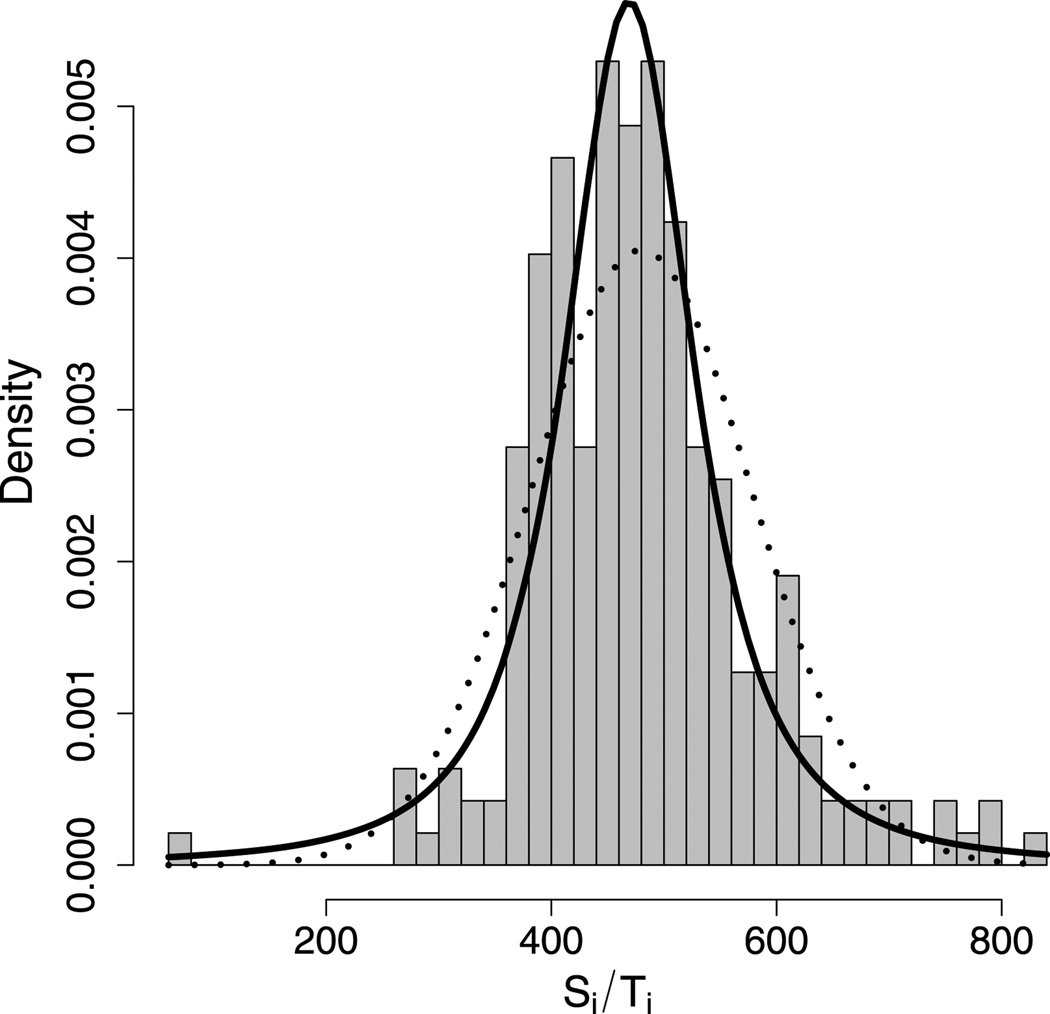
Figure 3 shows a histogram of experimentally observed single-molecule run length (nm) and run time (s) data for kinesin-2 (with n = 236) collected at the Hancock Lab at Penn State (Shastry and Hancock 2011). The probability densities shown in the figure correspond to the fitted Pearson (see Section 3) and normal distributions. The data appear to be in closer agreement with the fitted Pearson type VII distribution than with the fitted normal distribution.

Figure 3.

A histogram of the experimental data along with two densities. The solid curve is the 𝒫 density with μ= μ̂_n and σ = σ̂_n. The dotted curve is the normal density with μ = X̄_n and $\sigma =\sqrt{\sum {(X_i-{\mathrm{X̄}}_n)}^2/(n-1)}$.

We support this conclusion by testing the null hypothesis that the data came from a normal distribution with estimated parameters. We denote the sample of velocities as X = (X₁ = S₁/T₁, …, X_n = S_n/T_n)′, where S_i and T_i are the total displacement and travel time for the ith motor. We tested the hypothesis using a Monte Carlo Lilliefors-type test (Lilliefors 1967), i.e., by parametric bootstrapping a Kolmogorov–Smirnov statistic (Shao 2003, pp. 446–449) for the fitted normal distribution.

More specifically, we used the test statistic

$$D_n^{+}(F)=\underset{i\in \{1,\mathrm{\dots },n\}}{\text{max}}\{i/n-F(X_{(i)})\},$$

where F is the 𝒩(X̄_n, ∑(X_i − X̄_n)²/(n − 1)) cdf and X_(i) is the ith order statistic of the sample. We used a Monte Carlo sample size of b = 1,000,000 to estimate the distribution of the statistic. Using the bootstrap sample, we compute the p value as

$$\frac{{\sum }_{j=1}^b\mathbf{1}\{{(D_n^{+}(F))}^{(j)}>D_n^{+}(F)\}}{b},$$

where 1 denotes the indicator function and $\{{(D_n^{+}(F))}^{(1)},\dots ,{(D_n^{+}(F))}^{(b)}\}$ is the bootstrap sample. The p value was 0.0468 (SE = 0.0002), and so we conclude that X probably did not come from the normal distribution.

We repeated this procedure using the fitted 𝒫 distribution as the null. The resulting p value was 0.618 (SE = 0.0005), and so we fail to reject the null hypothesis that the sample came from the 𝒫(μ̂_n, σ̂_n) distribution.

Although our limit theorem and these hypothesis tests are compelling, it would be ideal if we could confirm that our experimental data did in fact arise from a distribution with infinite variance. In an effort to do so, we conducted an extreme-value analysis of the data, based on the generalized Pareto distribution (GPD) (Coles 2001). The analysis proved inconclusive due to the small sample size. A simulation study, in which we simulated larger samples from the fitted 𝒫 distribution, showed that a sample size of at least 400 would be needed to produce a sufficiently narrow confidence interval for the GPD shape parameter.

3. MAXIMUM LIKELIHOOD INFERENCE FOR THE 𝒫 DISTRIBUTION

In this section we develop maximum likelihood inference for the 𝒫 distribution and consider the one- and two-sample location problems.

3.1. One-Sample Inference

First we derive the 𝒫 quantile function because we will need it in order to find a consistent estimator of σ. We begin by finding the 𝒫 distribution function. We have

$$F(x)=\frac{1}{2\sigma }{\int }_{-\infty }^x{(1+{\left(\frac{t-\mu }{\sigma }\right)}^2)}^{-3/2}dt,$$

which can be simplified slightly by making the substitution y = (t − μ)/σ. This yields

$$F(x)=\frac{1}{2}{\int }_{-\infty }^{\frac{x-\mu }{\sigma }}{(1+y^2)}^{-3/2}dy.$$

Now, let z = arctan((t − μ)/σ) so that

$$F(x)=\frac{1}{2}{\int }_{-\pi /2}^{\text{arctan}\frac{x-\mu }{\sigma }}\text{cos}zdz=\frac{1}{2}(\text{sin arctan}\frac{x-\mu }{\sigma }-\text{sin}(-\pi /2))=\frac{1}{2}(1+\frac{x-\mu }{\sqrt{{\sigma }^2+{(x-\mu )}^2}}).$$

Thus the quantile function is

$$F^{-1}(y)=\mu +\frac{\sigma }{2}\frac{2y-1}{\sqrt{y(1-y)}}.$$

Now, let X = (X₁, …, X_n) be i.i.d. 𝒫(μ, σ) random variables, and let θ = (μ, σ)′. Then the likelihood of θ given X = x is

$$L_n(\mathit{\theta }|\mathit{x})\propto {\sigma }^{-n}\prod _i{(1+{\left(\frac{x_i-\mu }{\sigma }\right)}^2)}^{-3/2},$$

which implies the log likelihood

$${\ell }_n(\mathit{\theta }|\mathit{x})=-n\text{log}\sigma -\frac{3}{2}\sum _i\text{log}(1+{\left(\frac{x_i-\mu }{\sigma }\right)}^2).$$

This likelihood is unimodal (Gabrielsen 1982), but optimization of ℓ_n may require many iterations or converge prematurely if starting values are chosen naively. And so we recommend that (μ, σ)′ be estimated using the following approach.

Let MED_n be the sample median of X and MAD_n be the sample median absolute deviation from the median, i.e., MAD_n = median{|X_i − MED_n|}. It can be shown, using a result from Serfling and Mazumder (2009), that (MED_n, MAD_n)′ is an $\sqrt{n}$-consistent estimator of (μ, MAD)′, where MAD is the population median absolute deviation from the median.

But we need an estimator of σ, i.e., we need k such that k · MAD = σ. Since the MAD is defined as the 75th percentile of the centered distribution, we have

$$\mathrm{M}\mathrm{A}\mathrm{D}=F_{X-\mu }^{-1}(3/4)=\sigma /\sqrt{3},$$

and so $k=\sqrt{3}$ for the 𝒫 distribution. Hence, ${\mathit{\theta ̃}}_n=({\mathrm{\mu ̃}}_n,{\mathrm{\sigma ̃}}_n)\prime =(\mathrm{M}\mathrm{E}{\mathrm{D}}_n,\sqrt{3}\mathrm{M}\mathrm{A}{\mathrm{D}}_n)\prime$ is $\sqrt{n}$-consistent for (μ, σ)′ by Slutsky’s theorem. We use θ̃_n as the starting value and find the MLE θ̂_n by iterating

$${\mathit{\theta }}^{(k+1)}={\mathit{\theta }}^{(k)}-{[{\nabla }^2{\ell }_n({\mathit{\theta }}^{(k)})]}^{-1}\nabla {\ell }_n({\mathit{\theta }}^{(k)})$$ (3.1)

until convergence, which generally requires only several iterations. The right-hand side of (3.1) is easy to compute because the second term has the simple form

$${[{\nabla }^2{\ell }_n(\mathit{\theta })]}^{-1}\nabla {\ell }_n(\mathit{\theta })={\left(\begin{array}{cc}\hfill 3\sum \frac{y^2-{\sigma }^2}{{({\sigma }^2+y^2)}^2}\hfill & \hfill -6\sigma \sum \frac{y}{{({\sigma }^2+y^2)}^2}\hfill \\ \hfill -6\sigma \sum \frac{y}{{({\sigma }^2+y^2)}^2}\hfill & \hfill \frac{n}{{\sigma }^2}-3\sum \frac{3y^2+y^4/{\sigma }^2}{{({\sigma }^2+y^2)}^2}\hfill \end{array}\right)}^{-1}\left(\begin{array}{c}\hfill 3\sum \frac{y}{{\sigma }^2+y^2}\hfill \\ \hfill -\frac{n}{\sigma }+3\sum \frac{y^2/\sigma }{{\sigma }^2+y^2}\hfill \end{array}\right),$$

where y represents x_i − μ. The variance of θ̂_n can then be estimated using the inverse of the observed Fisher information matrix [−∇²ℓ_n(θ̂_n)]⁻¹.

3.2. The One-Sample Location Problem

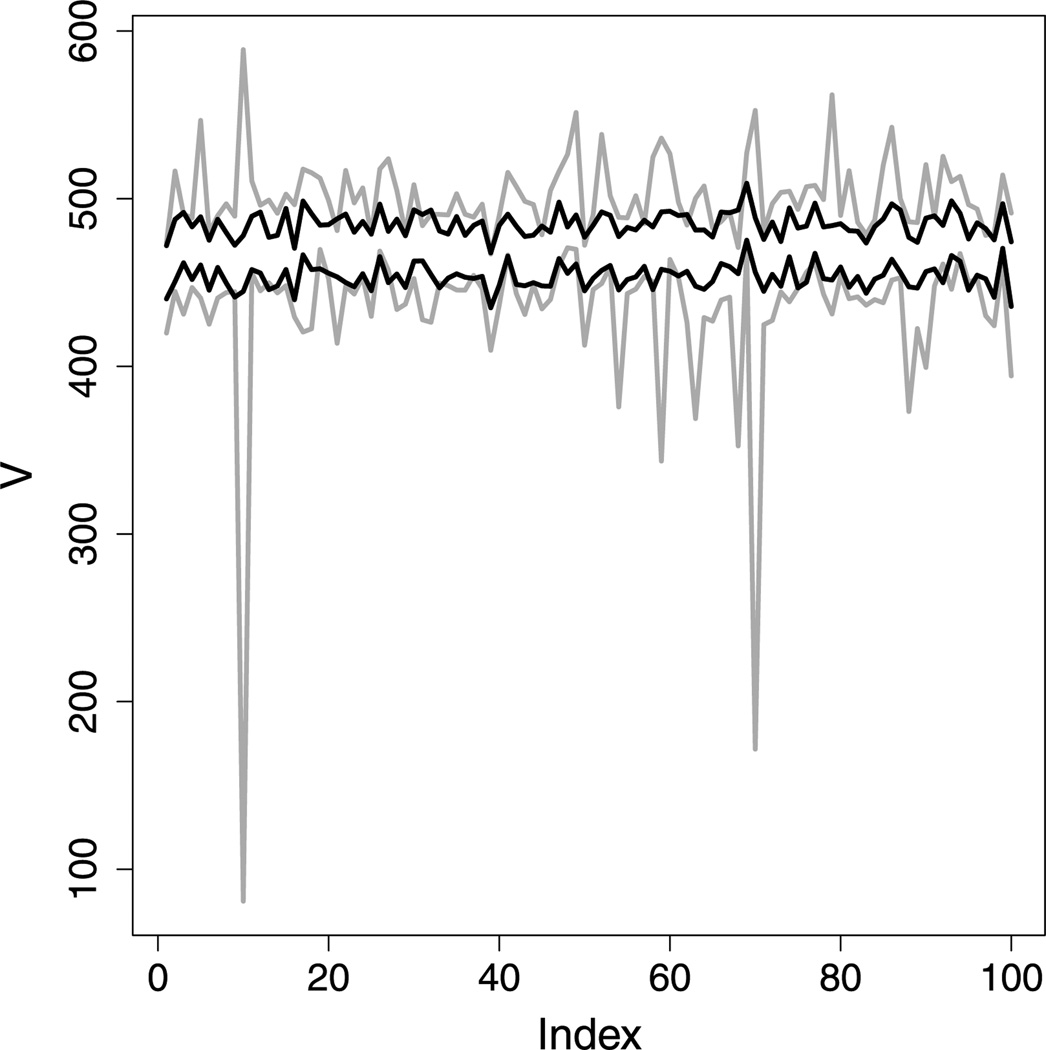
The plot in Figure 4 shows how the widths of confidence intervals for velocity differ depending on the assumption of 𝒫 data or the assumption of normality. The intervals shown are 95 % intervals for 100 samples from the 𝒫 distribution with μ = 469 and σ = 88 (the estimates for the data set analyzed in Section 2.4). Each sample had size 100, which is realistic.

Figure 4.

The t-based and Pearson confidence intervals for 100 data sets simulated from the 𝒫(469, 88) distribution. The extents of the Pearson intervals are shown in black, the t intervals in gray. For this study, the t intervals were just over twice as wide, on average, as the Pearson intervals.

Although t-based inference offers the desired coverage and excellent power for this scenario, we see that the t-based intervals tend to be much wider than the Pearson intervals—over twice as wide, on average, for this simulation (cf. Table 1). And a t-based interval may be almost arbitrarily wide for a given data set, owing to the sensitivity of the sample variance to extreme observations. Indeed, quite a few of the t-based intervals shown in Figure 4 are extremely wide (as wide as 510).

Table 1.

Coverage rates, mean CI widths, and maximum CI widths for the one-sample simulation study.

Assumption	Coverage rate	Mean CI width	Maximum CI width
Pearson	97 % (0.02)	31.8 (0.3)	39.6
Normal	95 % (0.02)	69.9 (6.0)	510.1

3.3. The Two-Sample Location Problem

A number of groups have engineered kinesins with extended neck linkers and measured the resulting change in the transport characteristics of the motors. For example, Muthukrishnan et al. (2009) and Shastry and Hancock (2010) found that extending the kinesin-1 neck linker by just a few amino acids significantly reduced processivity. And Yildiz et al. (2008) inserted up to 26 proline residues into the neck linker of human kinesin-1 and measured the speed, run length, and various other characteristics of the mutant motors. They found that a longer neck linker reduces the speed of a motor and permits larger forward and backward steps.

If researchers hope to engineer motors with “fine tuned” functional characteristics, they must be able to measure small changes in function that result from a given change in motor structure. In the current context, this means being able to measure small changes in velocity that result from changes in neck linker length.

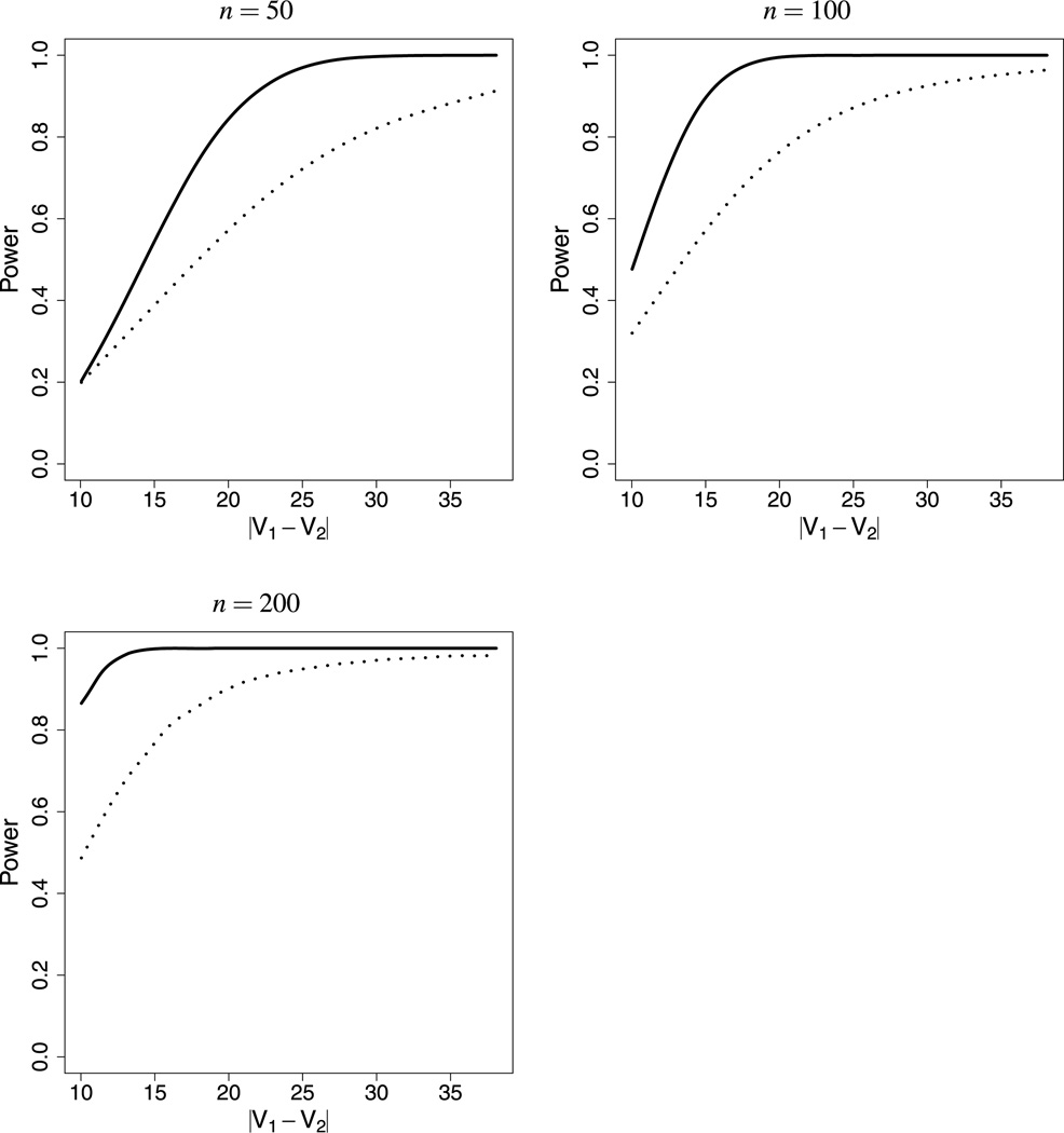
The plots in Figure 5 show the results of a simulation study designed to determine whether the assumption of normality can undermine one’s ability to resolve a small difference in the velocities of two types of motors when the data are in fact 𝒫 distributed. The study used biologically relevant values of D, μ_τ, μ_z, and m (Hughes, Hancock, and Fricks 2012).

Figure 5.

The power to resolve a difference in velocities when the data are 𝒫 distributed, for sample sizes 50, 100, and 200. The solid curve shows the power when one correctly assumes 𝒫-distributed data. The dotted curve shows the power if one incorrectly assumes that the data are normal, i.e., if one applies Welch’s t test.

The figure shows a plot for each of three realistic sample sizes: 50, 100, and 200. If we assume normality, the appropriate statistic is Welch’s t. For the assumption of Pearson data, we used a Wald test based on the statistic

$$\frac{{\mathrm{\mu ̂}}_1-{\mathrm{\mu ̂}}_2}{\sqrt{\mathrm{𝕍̂}{\mathrm{\mu ̂}}_1+\mathrm{𝕍̂}{\mathrm{\mu ̂}}_2}}.$$

We see from the plots that Welch’s t test has less power to resolve small differences in motor velocity when the data are 𝒫 distributed.

3.4. Two-Sample Inference for Experimental Data

Table 2 shows that these different assumptions can make a difference for analyses of experimental data. The two samples are single-molecule data collected for human kinesin-5 (KSP) motors that were engineered with shorter (14- and 15-amino acid) neck-linker domains to make them more processive (Shastry and Hancock 2011). (Kinesin-5 motors are known to slide microtubules apart during mitosis; see Goshima and Vale 2005.) At significance level 0.05, the Wald test rejects the hypothesis that the two motors have the same velocity. The t test, on the other hand, fails to reject.

Table 2.

Results from the analyses of two samples of data collected for two kinds of kinesin-5 motors. The first sample had 83 observations, the second sample 79.

	Sample 1		Sample 2
Assumption	μ1	σ1	μ2	σ2	Statistic	P value
Pearson	82.06 (79.07, 85.05)	15.65	89.64 (85.06, 94.24)	21.80	−2.71	0.0034
Normal	78.87 (70.18, 87.55)	39.57	85.53 (79.11, 91.95)	28.52	−1.23	0.22

4. CONCLUSION

In this paper we have developed methodology to better understand empirically measured velocity from molecular motor assays. Using a broad modeling framework that includes a large class of molecular motormodels, we have shown that empirical velocity has a limiting Pearson type VII distribution centered at the true velocity and having infinite variance. Moreover, we have been able to show experimental evidence of the validity of this scaling limit, thereby providing evidence for the validity of this type of model. This and similar scaling limits allow us to link phenomena at the scale of interest (the level of individual steps) to data observed at another scale, that of detachment after a relatively large number of steps.

We developed maximum likelihood inference for the relevant Pearson distribution and showed that, compared to the standard model (which assumes normality), our approach leads to more precise inference for velocity in the one-sample setting and offers more power to resolve small differences in velocity in the two-sample case. Hence, our approach will allow experimentalists to better determine the velocity of a given type of motor or to find a difference in velocity for two types of motors.

R (Ihaka and Gentleman 1996) code is available on the first author’s website.

REFERENCES

- Atzberger P, Peskin C. A Brownian Dynamics Model of Kinesin in Three Dimensions Incorporating the Force-Extension Profile of the Coiled-Coil Cargo Tether. Bulletin of Mathematical Biology. 2006;68:131–160. doi: 10.1007/s11538-005-9003-6. [DOI] [PubMed] [Google Scholar]
- Coles S. An Introduction to Statistical Modeling of Extreme Values. London: Springer; 2001. [Google Scholar]
- Devroye L. Non-Uniform Random Variate Generation. New York: Springer; 1986. [Google Scholar]
- Elston T, Peskin C. The Role of Protein Flexibility in Molecular Motor Function: Coupled Diffusion in a Tilted Periodic Potential. SIAM Journal on Applied Mathematics. 2000;60:842–867. [Google Scholar]
- Gabrielsen G. On the Unimodality of the Likelihood for the Cauchy Distribution: Some Comments. Biometrika. 1982;69:677–678. [Google Scholar]
- Goshima G, Vale RD. Cell Cycle-Dependent Dynamics and Regulation of Mitotic Kinesins in Drosophila S2 Cells. Molecular Biology of the Cell. 2005;16:3896–3907. doi: 10.1091/mbc.E05-02-0118. [DOI] [PMC free article] [PubMed] [Google Scholar]
- Hirokawa N, Takemura R. Biochemical and Molecular Characterization of Diseases Linked to Motor Proteins. Trends in Biochemical Sciences. 2003;28:558–565. doi: 10.1016/j.tibs.2003.08.006. [DOI] [PubMed] [Google Scholar]
- Hirokawa N, Pfister KK, Yorifuji H, Wagner MC, Brady ST, Bloom GS. Submolecular Domains of Bovine Brain Kinesin Identified by Electron Microscopy and Monoclonal Antibody Decoration. Cell. 1989;56:867–878. doi: 10.1016/0092-8674(89)90691-0. [DOI] [PubMed] [Google Scholar]
- Hughes J, Hancock WO, Fricks J. A Matrix Computational Approach to Kinesin Neck Linker Extension. Journal of Theoretical Biology. 2011;269:181–194. doi: 10.1016/j.jtbi.2010.10.005. [DOI] [PubMed] [Google Scholar]
- Hughes J, Hancock WO, Fricks J. Kinesins with Extended Neck Linkers: A Chemomechanical Model for Variable-Length Stepping. Bulletin of Mathematical Biology. 2012;74:1066–1097. doi: 10.1007/s11538-011-9697-6. [DOI] [PMC free article] [PubMed] [Google Scholar]
- Ihaka R, Gentleman R. R: A Language for Data Analysis and Graphics. Journal of Computational and Graphical Statistics. 1996;5:299–314. [Google Scholar]
- Kolomeisky A, Fisher M. Molecular Motors: A Theorist’s Perspective. Annual Review of Physical Chemistry. 2007;58:675–695. doi: 10.1146/annurev.physchem.58.032806.104532. [DOI] [PubMed] [Google Scholar]
- Kural C, Balci H, Selvin PR. Molecular Motors One at a Time: Fiona to the Rescue. Journal of Physics. Condensed Matter. 2005;17:S3979–S3995. doi: 10.1088/0953-8984/17/47/023. [DOI] [PubMed] [Google Scholar]
- Kutys M, Fricks J, Hancock W. Monte Carlo Analysis of Neck Linker Extension in Kinesin Molecular Motors. PLoS Computational Biology. 2010;6:e1000980. doi: 10.1371/journal.pcbi.1000980. [DOI] [PMC free article] [PubMed] [Google Scholar]
- Lilliefors H. On the Kolmogorov–Smirnov Test for Normality with Mean and Variance Unknown. Journal of the American Statistical Association. 1967;62:399–402. [Google Scholar]
- Miki H, Setou M, Kaneshiro K, Hirokawa N. All Kinesin Superfamily Protein, KIF, Genes in Mouse and Human. Proceedings of the National Academy of Sciences of the United States of America. 2001;98:7004–7011. doi: 10.1073/pnas.111145398. [DOI] [PMC free article] [PubMed] [Google Scholar]
- Mogilner A, Wang H, Elston T, Oster G. Molecular Motors: Theory and Experiment. In: Fall C, Marland E, Wagner J, Tyson J, editors. Computational Cell Biology. New York: Springer; 2002. [Google Scholar]
- Muthukrishnan G, Zhang Y, Shastry S, Hancock W. The Processivity of Kinesin-2 Motors Suggests Diminished Front-Head Gating. Current Biology. 2009;19:442–447. doi: 10.1016/j.cub.2009.01.058. [DOI] [PMC free article] [PubMed] [Google Scholar]
- Pearson K. Contributions to the Mathematical Theory of Evolution. II. Skew Variation in Homogeneous Material. Philosophical Transactions of the Royal Society of London, Series A: Mathematical and Physical Sciences. 1895;186:343–414. [Google Scholar]
- Pearson K. Mathematical Contributions to the Theory of Evolution. X. Supplement to a Memoir on Skew Variation. Philosophical Transactions of the Royal Society of London, Series A: Mathematical and Physical Sciences. 1901;197:443. [Google Scholar]
- Pearson K. Mathematical Contributions to the Theory of Evolution. XIX. Second Supplement to a Memoir on Skew Variation. Philosophical Transactions of the Royal Society of London, Series A: Mathematical and Physical Sciences. 1916;216:429–457. [Google Scholar]
- Serfling R, Mazumder S. Exponential Probability Inequality and Convergence Results for the Median Absolute Deviation and Its Modifications. Statistics & Probability Letters. 2009;79:1767–1773. [Google Scholar]
- Shao J. Mathematical Statistics. Berlin: Springer; 2003. [Google Scholar]
- Shastry S, Hancock WO. Neck Linker Length Determines the Degree of Processivity in Kinesin-1 and Kinesin-2 Motors. Current Biology. 2010;20:939–943. doi: 10.1016/j.cub.2010.03.065. [DOI] [PMC free article] [PubMed] [Google Scholar]
- Shastry S, Hancock WO. Interhead Tension Determines Processivity Across Diverse n-Terminal Kinesins. Proceedings of the National Academy of Sciences of the United States of America. 2011;108:16253–16258. doi: 10.1073/pnas.1102628108. [DOI] [PMC free article] [PubMed] [Google Scholar]
- Spudich JA, Rice SE, Rock RS, Purcell TJ, Warrick HM. Optical Traps to Study Properties of Molecular Motors. Cold Spring Harbor Protocols. 2011:2011. doi: 10.1101/pdb.top066662. [DOI] [PMC free article] [PubMed] [Google Scholar]
- Whitt W. Stochastic-Process Limits: An Introduction to Stochastic-Process Limits and Their Application to Queues. Berlin: Springer; 2002. [Google Scholar]
- Yang JT, Laymon RA, Goldstein LS. A Three-Domain Structure of Kinesin Heavy Chain Revealed by DNA Sequence and Microtubule Binding Analyses. Cell. 1989;56:879–889. doi: 10.1016/0092-8674(89)90692-2. [DOI] [PubMed] [Google Scholar]
- Yildiz A, Tomishige M, Gennerich A, Vale R. Intramolecular Strain Coordinates Kinesin Stepping Behavior Along Microtubules. Cell. 2008;134:1030–1041. doi: 10.1016/j.cell.2008.07.018. [DOI] [PMC free article] [PubMed] [Google Scholar]