Dynamic Active Contours for Visual Tracking

Abstract

Visual tracking using active contours is usually set in a static framework. The active contour tracks the object of interest in a given frame of an image sequence. A subsequent prediction step ensures good initial placement for the next frame. This approach is unnatural; the curve evolution gets decoupled from the actual dynamics of the objects to be tracked. True dynamical approaches exist, all being marker particle based and thus prone to the shortcomings of such particle-based implementations. In particular, topological changes are not handled naturally in this framework. The now classical level set approach is tailored for evolutions of manifolds of codimension one. However, dynamic curve evolution is at least a codimension two problem. We propose an efficient, level set based approach for dynamic curve evolution, which addresses the artificial separation of segmentation and prediction while retaining all the desirable properties of the level set formulation. It is based on a new energy minimization functional which, for the first time, puts dynamics into the geodesic active contour framework.

I. Introduction

Object tracking can be accomplished in many ways including by mechanical, acoustical, magnetic, inertial, or optical sensing, and by radio and microwaves, to mention a few. The ideal tracker should be “tiny, self-contained, complete, accurate, fast, immune to occlusions, robust, tenacious, wireless, and cheap” [1], [2]. As of now such a tracker does not exist; tradeoffs are necessary, and a method should be chosen based on the application in mind. Optical sensing is unobtrusive and can be simplified by choosing a simple (possibly prespecified) work environment, or by altering the appearance of the objects to be tracked (e.g., by painting them, or by mounting light sources on them). The desired objects to be tracked then become much easier to detect. However, in certain instances (e.g., for an uncooperative object to be followed) this is not possible. Visual tracking is the task of following the positions of possibly multiple objects based on the inputs of one or many cameras (the optical sensors). In the context of visual tracking, we can distinguish between the two tasks of locating and following an object (e.g., for surveillance applications), and influencing objects or our environment (e.g., controlling the movement of a plane, based on visual input). The latter will most likely encompass the first (possibly resulting in nested control loops). Both tasks can be accomplished by means of feedback mechanisms. In either case we need a good estimate of object position. Once we have this estimation, we either have fulfilled our task (e.g., for surveillance applications), or use this information to close a control loop. This brings to mind a broad range of applications. Indeed, be it for medical or military use, the need for visual tracking is ubiquitous.

Visual feedback control differs significantly from classical control. Sensors are imaging devices (usually cameras) which deliver an abundance of information of which only a fraction may be needed for a specific control task. The sensor output needs to be preprocessed to extract the relevant information for the tracking problem, e.g., the position of an object to be followed. Preprocessing usually encompasses noise-suppression (e.g., image smoothing) and segmentation to delineate objects from their background and from each other. Segmentation has been an active field of study in various application areas, most prominently in the medical sciences. Static segmentation problems are challenging. Segmentation algorithms usually need to be adapted to the problem at hand. There is no omnipotent segmentation algorithm. Visual tracking is a dynamic segmentation problem, where segmentations change over time. Here, additional information (e.g., apparent image motion) is available, but further degrees of freedom and thus difficulties are introduced, for example related to processing speed in real-time applications. Visual tracking poses various interesting questions to control theoreticians and engineers, among others:

• How can one properly deal with the unusual sensor signal, i.e., image information, projections on the image plane, correspondences for stereo vision, etc.?

• How should uncertainties be modeled? In most cases only very simple motion and system models are available. Delays may be significant in case of computationally demanding tracking algorithms.

• How should robustness or tracking quality be quantified? For example, what is the most suitable metric for the space of curves?

Humans and animals perform visual tracking tasks with ease every day: Following cars in traffic, watching other people, following the lines of text in a document, etc. These mundane tasks seem simple, but robust reliable algorithms and their computer implementation have proven to be quite challenging [3]. We rely on a highly developed brain, assumptions about the world acquired throughout a lifetime, and our eyes as visual sensors. The design of algorithms which would make a machine behave and perceive similarly to humans in all situations is a daunting task which is far from being solved. However, if we are only interested in a specific application, the problem becomes more tractable. Visual tracking is a relatively well defined problem when dealing with well defined environments.¹

Applications for visual tracking are diverse. Some key areas of research include the following.

• Vehicle guidance and control: See [4]–[9] for applications to autonomous driving.² See Sinopoli et al. [10] and Sharp et al. [11] for visual tracking systems for the navigation and the landing of an unmanned aerial vehicle, respectively.

• Surveillance and identification: See [12]–[14] for applications to target tracking and biometric identification.

• Robotics/Manufacturing: See Corke [15] and Hutchinsion et al. [16] for discussions on visual servo control which requires the visual tracking of objects/object features as a preprocessing stage. Here visual tracking is used to increase the bandwidth and accuracy of robots. We note that visual grasping falls into this category of tasks.

• User interfaces: See [17] for real-time fingertip tracking and gesture recognition, and [3] for virtual environments.

• Video processing: See [18] for automated addition of virtual objects to a movie.

• Medical applications: See [19] for applications to vision guided surgery (surgical instrument tracking) and [20] for medical image tracking.

A wide variety of algorithms for visual tracking exists, e.g., feature trackers, blob trackers, contour/surface trackers. See [21]–[26], and the references therein. All of these have their own advantages and disadvantages. The seminal paper of Kass et al. [27] spawned a huge interest in the area of contour/surface tracking algorithms. This is the class of algorithms on which we will focus in this paper.

II. Problem Statement, Motivation, and Scope

Typical geometric active contours [28]–[32] are static. However, variational formulations many times appear to be dynamic because the resulting Euler–Lagrange equations are solved by gradient descent, introducing an artificial time parameter. This time parameter simply describes the evolution of the gradient descent. It will usually not be related to physical time. A two step approach is typically used for visual tracking by static active contours. First, the curve evolves on a static frame until convergence (or for a fixed number of evolution steps). Second, the location of the curve in the next frame is predicted. In the simplest case, this prediction is the current location. Better prediction results can be achieved by using optical flow information, for example. In this two step approach, the curve is not moving intrinsically, but instead is placed in the solution’s vicinity by an external observer (the prediction algorithm). The curve is completely unaware of its state. In contrast, Terzopoulos and Szeliski [33] or Peterfreund [34] view curve evolution from a dynamical systems perspective; both methods are marker particle based and are fast, but they may suffer from numerical problems (e.g., in the case of sharp corners [35]–[37]). In the static case, level set methods are known to handle sharp corners, topological changes, and to be numerically robust. In their standard form, they are restricted to codimension one problems, and thus not suitable for dynamic curve evolution. Extensions of level set methods to higher codimensions exist and a level set formulation for dynamic curve evolution is desirable [38], [39]. We will present a straightforward level set based dynamic curve evolution framework in this paper.

The results of this paper relate to dynamic snakes [33] as geodesic or conformal active contours [30], [29] relate to the original snake formulation [27]. Here we are advocating a different philosophy to dynamic curve evolution. Instead of discretizing evolution equations upfront (early lumping), we keep the partial differential equations as long as possible (late lumping [40]), resulting in a more natural and geometric formulation.

We demonstrate that we can attach information to a contour evolving in a level set framework. This is related to the approach in [41] and is a crucial step toward more flexible level set based approaches. Most level set based evolution equations in image processing are static and/or do not possess state information. This can be a major drawback, e.g., if we want to follow a contour portion over time.

Error injection is a standard method from control theory to construct observers. All snakes using an observer (e.g., Kalman filter-based or particle filter-based) use error injection. Observers for marker particle based systems are finite dimensional. Our proposed approach requires an observer for an infinite dimensional, nonlinear system. The existing theory for such systems is still in its infancy; system theoretic results are available only in special cases. We restrict ourselves to error injection resembling a nonlinear, infinite dimensional observer if we are close enough to the basin of attraction of the object of interest. The incorporation of the optical flow constraint is natural in this framework. Our formulation restricts the propagation to the direction normal to the object direction; this is exactly measured by the optical flow, in contrast to previous approaches [33] for dynamic snakes which do not restrict the direction of movement. Thus, even though error injection is classical, it is novel in this level set framework.

We now briefly summarize the contents of the remaining sections of this paper. Section III gives a brief overview over existing methods for contour based visual tracking. Section IV introduces the concept of static curve evolution and positions it in relation to classical image processing. Section V reviews the fundamentals of parameterized dynamic curve evolution. Section VI introduces geometric dynamic curve evolution and discusses the evolution equations. The level set formulation for normal geometric dynamic curve evolution is given in Section VII. Sections VIII and X deal with error injection into the evolution equations and occlusion detection, respectively. Simulation results obtained on real image sequences are presented in Section XI. Section XII discusses our results and future work. We also include some appendices with the derivations of the key formulas.

III. Alternative Contour-Based Tracking Methodologies

The literature on tracking is vast. To give a complete overview on tracking methodologies is beyond the scope of this paper. We limit ourselves to a brief overview of the (what we think) closest approaches, i.e., contour based tracking methodologies, highlighting their differences.³

A possible classification for contour based trackers is based on

• the motion model: finite dimensional (parametric) or infinite dimensional;

• the curve model: finite dimensional, or infinite dimensional;

• the solution method: optimization, or integration in time;

• the type of curve influence terms (boundary, area, statistics, etc.).

Most visual tracking approaches employ finite dimensional motion models and finite dimensional curve evolution models. If the curve change over time is only described by the motion model (the motion group), i.e., if there is no change of the curve shape and consequently no curve evolution model, curve based trackers can easily be cast as finite dimensional observation problems. Approaches include all flavors of the Kalman filter (“classical” Kalman filter, extended Kalman filter, unscented Kalman filter or sigma point filter), probability data association filters, and particle filters [42]. Finite-dimensional motion groups are usually chosen to be translation, translation plus rotation, or the affine transformation group.

Extending these finite dimensional filtering methods to elastic deformations is generally not straightforward, since the evolution equations or observations tend to be nonlinear. One approach is to parameterize the curve shape. This can for example be done by Fourier modes, principal component analysis, or in the simplest possible case by a piecewise linear approximation of the boundary (a particle-based method). In the latter dynamic case [33], [34], [43], the boundary is represented by a prespecified number of points plus their associated velocities. Increasing the degrees of freedom has the disadvantage of increasing the computational complexity. This is particularly true for particle filtering approaches, which can only handle a moderate number of states without becoming computationally intractable. Also, parameterizing a curve shape (independent of the type of parameterization used) introduces a strong shape bias: i.e., the shape is assumed to lie in a certain (prespecified) class. This may be desired in case of an object with clearly defined shape, but may be unwanted if objects are allowed to deform completely elastically.

Moving away from finite dimensional to infinite-dimensional curve representations results in great flexibility, but comes at the cost of less theoretical insight. Nonlinear infinite-dimensional curve evolution equations require nonlinear infinite-dimensional observers which are (unlike observers for linear systems) understood only for special system classes.

Infinite-dimensional curve descriptions have been used in combination with the trivial motion model [27] (i.e., no dynamic motion is assumed, all shape changes are purely static), in combination with finite dimensional motion models [44]–[47], as well as in combination with infinite-dimensional motion models [48], [49]. Since finite-dimensional motion models cannot account for arbitrary elastic deformations they are frequently combined with an elastic update step: this is called deformotion in [45] and employed for tracking purposes in conjunction with a simple observer structure in [47] and in a particle-filtering framework in [44]. Particle-filtering [42] has been very popular in the computer vision community, but is usually restricted to low-dimensional state spaces to keep the computational cost reasonable. In [42], an affine motion model is used, there is no elastic deformation of the curve. Rathi et al. [44] extend the particle-filtering approach to include elastic curve deformation in the observer update step. However, the state space is not truly infinite-dimensional, in particular there is no infinite-dimensional motion model.

Approaches using infinite-dimensional motion models for visual tracking usually employ some form of passive advection, e.g., the curve gets pushed forward through an external vector field for example established through an optical flow computation [48] or through a motion segmentation step [49].

In this paper, we are interested in adding dynamics to the curve evolution itself, so that it is no longer passively advected, but possesses an intrinsic velocity associated with every point on the curve. The approach taken is to construct an infinite-dimensional dynamically evolving curve based on the ideas by Terzopoulos [33]. It is a dynamical systems viewpoint which does not require static optimization steps as in many other approaches.

IV. Static Curve Evolution

Image processing in the line of traditional signal processing is concerned with low-level vision tasks: e.g., performing image denoising, edge detection, deconvolutions, etc. In this setting images are treated as multidimensional signals, and there are usually no high-level assumptions regarding the image content (e.g., looking specifically to find an object of specific texture, etc.). On the other side of the spectrum is high-level vision (high-level reasoning) which tries to address the latter problem of what is represented in an image. The image is to be decomposed into meaningful subparts (the process of segmentation; e.g., foreground, background, uniform regions) which are subsequently analyzed (e.g., which types of objects do the segmented regions correspond to). Creating such a high-level vision system is a tremendously hard task, far from being solved. Tasks that are straightforward for humans turn out to be strikingly difficult in the algorithmic setting of computers, requiring assumptions about and simplifications of the vision problem to be approached. There is no segmentation algorithm that works for all cases. A popular simplification is to assume that objects in an image are separated from their background, for example by intensity edges, variations in image statistics, color, etc. Template matching is a common approach for image segmentations of known objects. Unfortunately, while robust, template matching is also inherently inflexible. If the image represents anything not accounted for in the template (e.g., an additional protrusion in the shape of the object) the template will not be able to capture it. Solid objects may be described by their interior, or (if only the shape outline is sufficient) by their boundary curves. Boundary descriptions are the vantage point for segmentations by curve evolution. The assumption here is that whatever object we are looking to segment may be described by a closed curve representing its boundary. Kass et al. [27] introduced what is known as the classical snake model for curve based segmentation. The basic idea is to minimize an energy functional depending on image influences (i.e., attracting it to edges) and curve shape. Given a parameterized curve in the plane of the form : S¹ × [0, θ) ↦ ℝ², where (p, θ) = [x(p, θ), y(p, θ)]^T ∈ C^2,1, p ∈ [0, 1] is the parameterization, $\theta \in {\mathbb{R}}_0^{+}$, (0, θ) = (1, θ) (i.e., the curve is closed), and θ is an artificial time, the energy

$$L(\mathcal{C},{\mathcal{C}}_p,{\mathcal{C}}_{pp})={\int }_0^1\underset{\text{elasticity}}{\underbrace{\frac{1}{2}{w}_1(p){\left|\right|{\mathcal{C}}_p\left|\right|}^2}}+\underset{\text{rigidity}}{\underbrace{\frac{1}{2}{w}_2(p){\left|\right|{\mathcal{C}}_{pp}\left|\right|}^2}}+\underset{\text{image}\text{influence}}{\underbrace{g(\mathcal{C})}}dp$$ (1)

is minimized, where w₁(p) and w₂(p) are parameterization dependent design parameters (usually set constant) and g ≥ 0 is some potential function (with the desired location of forming a potential well). A common choice for the potential function is

$$g(\mathit{x})=\frac{1}{1+{\left|\right|G\ast \nabla I(\mathit{x})\left|\right|}^r}$$

where x =[x, y]^T denotes image position, I is the image intensity, r is a positive integer, and G is a Gaussian. See Fig. 1 for an illustration of curve parameterization. In most applications, the rigidity term is disregarded (i.e., w₂(p) ≡ 0). The energy (1) is independent of time. It is a static optimization problem, which may be solved by means of calculus of variations. The corresponding Euler–Lagrange equation for the candidate minimizer of L( , , ) is

Fig. 1.

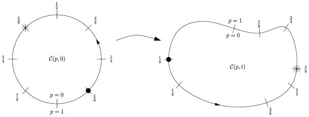
Parameterized curve evolution. The parametrization travels with a particle. In general, the parametrization will not stay uniformly spaced. The black disk and the asterisk indicate particles attached to the curve; their assigned value for p will stay the same throughout the evolution.

$$\mathbf{0}=\underset{\text{elasticity}\text{influence}}{\underbrace{-\frac{\partial }{\partial p}(w_1{\mathcal{C}}_p)}}+\underset{\text{rigidity}\text{influence}}{\underbrace{\frac{{\partial }^2}{\partial p^2}(w_2{\mathcal{C}}_{pp})}}+\underset{\text{image}\text{influence}}{\underbrace{\nabla g}}.$$ (2)

The right hand side of (2) can be interpreted as an infinite-dimensional gradient. Consequently, moving into the negative gradient direction results in the gradient descent solution scheme for (1)

$${\mathcal{C}}_{\theta }=\frac{\partial }{\partial p}(w_1{\mathcal{C}}_p)-\frac{{\partial }^2}{\partial p^2}(w_2{\mathcal{C}}_{pp})-\nabla g.$$ (3)

The solution of (1) is a tradeoff between the elasticity term (trying to shrink the curve length), the rigidity term (favoring straight curve segments), and the image influence term (trying to attract the curve for example to an intensity edge). The tradeoff implies that sharp corners are usually not represented well (unless they are coded explicitly into the method). Problematic with the original snake formulation is that it is not geometric, i.e., the derivatives do not represent clear geometric quantities (e.g., normals and curvature) and the solution depends on the somewhat arbitrary parameterization p. On the other hand, the geodesic active contour [48], [30], another curve-based segmentation method, is completely geometric. To understand the motivation behind the geodesic active contour it is instructive to look at the length minimizing flow first, i.e., the curve evolution that minimizes

$$L({\mathcal{C}}_p)={\int }_0^{l}ds={\int }_0^1\left|\right|{\mathcal{C}}_p\left|\right|dp$$

where s denotes arclength and l the length of the curve . The gradient descent scheme that minimizes curve length is

$${\mathcal{C}}_{\theta }=\kappa \mathcal{N}$$ (4)

where denotes the unit-inward normal to and κ = · is the signed curvature. Equation (4) is known as the geometric heat equation or the Euclidean curve shortening flow. Gage and Hamilton [50] proved that a planar embedded convex curve converges to a round point when evolving according to (4). (A round point is a point that, when the curve is normalized in order to enclose an area equal to π, is equal to the unit disk.) Grayson [51] proved that a planar embedded nonconvex curve converges to a convex one, and from there to a round point from Gage and Hamilton result. Note that in spite of the local character of the evolution, global properties are obtained, which is a very interesting feature of this evolution. For other results related to the Euclidean shortening flow, see [50]–[55]. The Euclidean curve shortening flow only depends on the curve shape. There is no image influence term. The idea of geodesic active contours is to introduce a conformal factor g( ) (in analogy to the potential function introduced above) into the energy functional, to minimize the weighted length⁴

$$L(\mathcal{C},{\mathcal{C}}_p)={\int }_0^{l}g(\mathcal{C})ds={\int }_0^{1}g(\mathcal{C})\left|\right|{\mathcal{C}}_p\left|\right|dp.$$ (5)

The gradient flow corresponding to (5) is

$${\mathcal{C}}_{\theta }=(g\kappa -(\nabla g·\mathcal{N}))\mathcal{N}.$$ (6)

Equation (6) only involves geometric terms, the curvature κ and the normal and is completely independent of parameterization. The term gκ is the geometric analog to the elasticity term (∂/∂p)(w₁ ) of (3) and the gradient term ∇g gets replaced by its projection onto . There is no correspondence to the rigidity term of the parametric snake, however this term is frequently discarded due to its fourth-order derivative. See [56] and [57] for more details. Many extensions to and variations of the active contour exist (e.g, adding an inflationary term). For more information, see [57] and the references therein.

Neither the snake (3) nor the geodesic active contour (6) are truly dynamic curve evolutions. In both cases only the steady state solution on a static image is sought. In visual tracking, objects move over time. Consequently tracking with closed curves implies estimating closed curves moving in space and time. This is not readily described by the snake or the geodesic active contour. Section V describes a dynamic extension to the parametric snake. However, the objective of this paper is the dynamic extension of the geodesic active contour which will be discussed in Section VI.

V. Parametrized Dynamic Curve Evolution

In this section, we review parameterized dynamic curve evolution [33]. We also introduce the mathematical setup required to derive the geometric dynamic curve evolution equations of Section VI.

We consider the evolution of closed curves of the form : S¹ × [0, τ) ↦ ℝ² in the plane, where = (p, t) and (0, t) = (1, t) [51], with t being the time, and p ∈ [0, 1] the curve’s parametrization (see Fig. 1 for an illustration). The classical formulation for dynamic curve evolution proposed by Terzopoulos and Szeliski [33] is derived by means of minimization of the action integral

$$\mathcal{L}={\int }_{t=t_0}^{t_1}L(t,\mathcal{C},{\mathcal{C}}_t)dt$$ (7)

where the subscripts denote partial derivatives (e.g., is the curve’s velocity). The Lagrangian, L = T − U, is the difference between the kinetic and the potential energy. The potential energy of the curve is the energy of the snake (1)

$$U={\int }_0^1\frac{1}{2}{w}_1{\left|\right|{\mathcal{C}}_p\left|\right|}^2+\frac{1}{2}{w}_2{\left|\right|{\mathcal{C}}_{pp}\left|\right|}^2+g(\mathcal{C})dp.$$

The kinetic energy is

$$T={\int }_0^1\frac{1}{2}\mu {\left|\right|{\mathcal{C}}_t\left|\right|}^{2}dp$$

where μ corresponds to mass per unit length. The Lagrangian is then

$$L={\int }_0^1\frac{1}{2}\mu {\left|\right|{\mathcal{C}}_t\left|\right|}^2-\frac{1}{2}{w}_1{\left|\right|{\mathcal{C}}_p\left|\right|}^2-\frac{1}{2}{w}_2{\left|\right|{\mathcal{C}}_{pp}\left|\right|}^2-g(\mathcal{C})dp.$$ (8)

Computing the first variation δ of the action integral (7) and setting it to zero yields the Euler–Lagrange equations for the candidate minimizer [58] in force balance form

$$\mu {\mathcal{C}}_{tt}=\frac{\partial }{\partial p}(w_1{\mathcal{C}}_p)-\frac{{\partial }^2}{\partial p^2}(w_2{\mathcal{C}}_{pp})-\nabla g.$$ (9)

Equation (9) depends on the parametrization p and is therefore not geometric (see Xu et al. [56] for a discussion on the relationship between parametric and geometric active contours). Our proposed methodology (see Section VI) will be completely independent of parametrization. It will be geometric.

VI. Geometric Dynamic Curve Evolution

In this section, we will present the geometric dynamic curve evolution equations, which evolve according to physically motivated time. These evolution equations constitute a geometric formulation of the parameterized dynamic approach reviewed in Section V in analogy with the connection between parameterized and geometric curve evolution described in Section IV. Minimizing (7) using the potential energy of the geodesic active contour (5)

$$U={\int }_0^{1}g(\mathcal{C})\left|\right|{\mathcal{C}}_p\left|\right|dp$$

and the kinetic energy

$$T={\int }_0^1\frac{1}{2}\mu {\left|\right|{\mathcal{C}}_t\left|\right|}^2\left|\right|{\mathcal{C}}_p\left|\right|dp$$

results in the Lagrangian

$$L={\int }_0^1\left(\frac{1}{2}\mu {\left|\right|{\mathcal{C}}_t\left|\right|}^2-g\right)\left|\right|{\mathcal{C}}_p\left|\right|dp.$$ (10)

Computing the first variation δL of the action integral (10) yields

$$\mu {\mathcal{C}}_{tt}=-\mu (\mathcal{T}·{\mathcal{C}}_{ts}){\mathcal{C}}_t-\mu ({\mathcal{C}}_t·{\mathcal{C}}_{ts})\mathcal{T}-\left(\frac{1}{2}\mu {\left|\right|{\mathcal{C}}_t\left|\right|}^2-g\right)\kappa \mathcal{N}-(\nabla g·\mathcal{N})\mathcal{N}$$ (11)

which is geometric and a natural extension of the geodesic active contour approach [29], [30] (see Appendix I for a derivation). Here is the unit inward normal, = ∂ /∂s the unit tangent vector to the curve, κ = · denotes curvature and s is the arclength parameter [59].

We can consider the term (gκ − ∇g · ) in (11) as a force exerted by the image potential g on the curve . Compare this to the evolution equation for geodesic active contours as given in [57] and [60] ( = (gκ − ∇g · ) ). From a controls perspective, this can be interpreted as a control law, based on g and its spatial gradient ∇g, which is designed to move the curve closer to the bottom of the potential well formed by g.

Equation (11) describes a curve evolution that is only influenced by inertia terms and information on the curve itself. To increase robustness the potential energy U can include region-based terms (see, for example, [61]–[63]). This would change the evolution (11), but such changes pose no problem to our proposed level set approach.

The state–space form of (11) is

$${\overline{\mathit{x}}}_t(s,t)={(\begin{array}{cccc}{x}_3(s,t)& x_4(s,t)& f_1(\mathit{x})& f_2(\mathit{x})\end{array})}^T$$ (12)

where x̄^T = [x₁, x₂, x₃, x₄]^T, x₁ = x(s, t), x₂ = y(s, t), x₃ = x_t(s, t), x₄ = y_t(s, t), and f_i are scalar functions in and x̄ its derivatives. The evolution describes the movement of a curve in ℝ⁴, where the geometrical shape can be recovered by the simple projection

$$\mathrm{\Pi }(\mathit{x})=\left(\begin{array}{c}{x}_1(s,t)\\ x_2(s,t)\end{array}\right).$$

A. Interpretation of the Evolution Terms for the Geometric Dynamic Curve Evolution

To get an understanding of (11) it is fruitful to look at the effect of its individual terms. The term

$$-(\nabla g·\mathcal{N})\mathcal{N}$$

accelerates the curve toward the potential well formed by g. Note that −∇g points toward the potential well. The term

$$-a(g,{\mathcal{C}}_t)\kappa \mathcal{N}=-\left(\frac{1}{2}\mu {\left|\right|{\mathcal{C}}_t\left|\right|}^2-g\right)\kappa \mathcal{N}$$

accelerates the curve based on its smoothness properties and

$$-\mu (\mathcal{T}·{\mathcal{C}}_{ts}){\mathcal{C}}_t$$ (13)

represents a smoothing term for the tangential velocity. We can decompose the velocity change at every point on the curve into its tangential and normal components as

$${\mathcal{C}}_{ts}=({\mathcal{C}}_{ts}·\mathcal{N})\mathcal{N}+({\mathcal{C}}_{ts}·\mathcal{T})\mathcal{T}.$$

We assume that the tangential and the normal components change approximately linearly close to the point of interest. A Taylor series expansion (at arclength s₀) yields

$$\begin{array}{l}({\mathcal{C}}_{ts}·\mathcal{N})(s)=({\mathcal{C}}_{ts}·\mathcal{N})(s_0)+{\frac{\partial ({\mathcal{C}}_{ts}·\mathcal{N})}{\partial s}|}_{s_0}(s-s_0)+\mathcal{O}(s^2)\\ =n_0+n_1(s-s_0)+\mathcal{O}(s^2)\\ ({\mathcal{C}}_{ts}·\mathcal{T})(s)=({\mathcal{C}}_{ts}·\mathcal{T})(s_0)+{\frac{\partial ({\mathcal{C}}_{ts}·\mathcal{T})}{\partial s}|}_{s_0}(s-s_0)+\mathcal{O}(s^2)\\ =t_0+t_1(s-s_0)+\mathcal{O}(s^2).\end{array}$$

In order to appreciate the effect of the term (13), it is sufficient to consider the two fundamental cases depicted in Figs. 2 and 3. The normal component (depicted in Fig. 2) is irrelevant for the evolution, since · = 0 in this case. The tangential component (depicted in Fig. 3) will counteract tangential gradients of . The two cases correspond to a linearly and a parabolically increasing velocity in the tangential direction. In both cases, the term −μ( · ) will counteract this tendency of tangentially diverging particles on the curve, ideally smoothing out the tangential velocities over the curve .

Fig. 2.

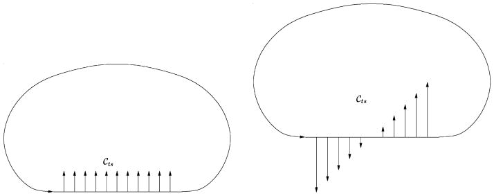
Normal direction, constant and linearly increasing.

Fig. 3.

Tangential direction, constant and linearly increasing.

The term

$$-\mu ({\mathcal{C}}_t·{\mathcal{C}}_{ts})\mathcal{T}$$

governs the transport of particles along the tangential direction. To understand what is occurring locally, we assume we are looking at a locally linear piece of the curve and decompose the velocity into

$${\mathcal{C}}_t=({\mathcal{C}}_t·\mathcal{T})\mathcal{T}+({\mathcal{C}}_t·\mathcal{N})\mathcal{N}.$$

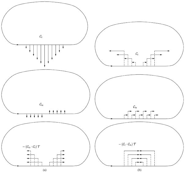
It is instructive to look at a triangular velocity shape in the normal direction [as shown in Fig. 4(a)] and in the tangential direction [as shown in Fig. 4(b)]. The triangular velocity shape in the normal direction induces a tangential movement of particles on the curve. This can be interpreted as a rubberband effect. Assume that the rubberband gets pulled at one point. This will elongate the rubberband. Since the point at which it is pulled stays fixed (no movement except for the displacement due to the pulling) particles next to it flow away from it. The triangular velocity shape in the tangential direction also induces tangential motion of the particles. However, this motion will counteract the initial tangential direction and will thus also lead to a smoothing effect on the change of tangential velocity vector over arclength.

Fig. 4.

Behavior of the term −μ( · ) . (a) Normal. (b) Tangential.

B. Normal Geometric Dynamic Curve Evolution

To get a quantitative interpretation of the behavior of the curve evolution (11), it is instructive to derive the corresponding evolution equations for the tangential and normal velocity components of the curve.

We can write

$${\mathcal{C}}_t=\alpha (p,t)\mathcal{T}+\beta (p,t)\mathcal{N}$$ (14)

where the parametrization p is independent of time and travels with its particle (i.e., every particle corresponds to a specific value p for all times), and α and β correspond to the tangential and the normal speed functions, respectively. By substituting (14) into (11) and using results from [64] (see Appendix II) we obtain the two coupled partial differential equations

$$\begin{array}{l}{\alpha }_t=-{({\alpha }^2)}_s+2\kappa \alpha \beta \\ {\beta }_t=-{(\alpha \beta )}_s+\left[\left(\frac{1}{2}{\beta }^2-\frac{3}{2}{\alpha }^2\right)+\frac{1}{\mu }g\right]\kappa -\frac{1}{\mu }\nabla g·\mathcal{N}.\end{array}$$ (15)

Here, −(α²)_s and −(αβ)_s are the transport terms for the tangential and the normal velocity along the contour, and gκ − ∇g · is the well known geodesic active contour image influence term [30], [29]. In contrast to the static geodesic active contour, this term influences the curve’s normal velocity rather than directly the curve’s position. It can be interpreted as a force. Finally, the terms 2καβ and ((1/2)β² − (3/2)α²)κ incorporate the dynamic elasticity effects of the curve. If we envision a rotating circle, we can interpret the term ((1/2)β² − (3/2)α²)κ as a rubberband (i.e., if we rotate the circle faster it will try to expand, but at the same time it will try to contract due to its then increasing normal velocity; oscillations can occur). If we restrict the movement of the curve to its normal direction (i.e., if we set α = 0) we obtain

$${\beta }_t=\frac{1}{2}{\beta }^2\kappa +\frac{1}{\mu }g\kappa -\frac{1}{\mu }\nabla g·\mathcal{N}.$$ (16)

This is a much simpler evolution equation. In our case it is identical to the full evolution (15) if the initial tangential velocity is zero. The image term g only influences the normal velocity evolution β. It does not create any additional tangential velocity. Thus, if α = 0 ∀s, then α = 0 ∀s, t; the flow with α = 0 is contained in (11) as an invariant subsystem. The restriction to curve movement in the normal direction is a design choice to simplify the approach. See Section VI-C for an illustration of the influence of a tangential velocity component.

If there is an initial tangential velocity, and/or if the image influence g contributes to the normal velocity β and to the tangential velocity α, the normal evolution equation will not necessarily be equivalent to the full evolution (15). We can always parametrize a curve such that the tangential velocity term vanishes. Specifically, if we consider a reparameterization

$$\overline{\mathcal{C}}(q,t)=\mathcal{C}(\phi (q,t),t)$$

where φ: ℝ × [0, T) ↦ ℝ, p = φ(q, t), φ_q > 0 then

$$\frac{\partial \overline{\mathcal{C}}}{\partial t}=\frac{\partial \mathcal{C}}{\partial t}+\frac{\partial \mathcal{C}}{\partial p}\frac{\partial \phi }{\partial t}.$$

The time evolution for C̄ can then be decomposed into

$${\overline{\mathcal{C}}}_t=\overline{\alpha }\mathcal{T}+\overline{\beta }\mathcal{N}=(\alpha (\phi (q,t),t)+||{\mathcal{C}}_p(\phi (q,t),t)||{\phi }_t)\mathcal{T}+\overline{\beta }\mathcal{N}$$

where

$$\begin{array}{l}\overline{\alpha }=\alpha (\phi (q,t),t)+\left|\right|{\mathcal{C}}_p(\phi (q,t),t)\left|\right|{\phi }_t\\ \overline{\beta }=\beta (\phi (q,t),t).\end{array}$$

If we choose φ as

$$\phi {(q,t)}_t=-\frac{\alpha (\phi (q,t),t)}{\left|\right|{\mathcal{C}}_p(\phi (q,t),t)\left|\right|}$$

we obtain

$${\overline{\mathcal{C}}}_t=\overline{\beta }\mathcal{N}$$

which is a curve evolution equation without a tangential component. For all times, t, the curve will move along its normal direction. However, the tangential velocity is still present in the update equation for β̄. After some algebraic manipulations, we arrive at

$$\mu ({\beta }_p{\phi }_t+{\beta }_t)=\left(\frac{1}{2}\mu {\beta }^2+g\right)\kappa -\nabla g·\mathcal{N}$$ (17)

which depends on the time derivative of the reparameterization function φ, which in turn depends on the tangential component α. The left-hand side of (17) represents a transport term along the curve, the speed of which depends on the time derivative of the reparameterization function φ.

C. Special Solutions

To illustrate the behavior of (15) and (16), we study a simple circular example. Assume g = μ = 1. Then ∇g = 0. Furthermore, assume that we evolve a circle with radius R and constant initial velocities

$$\alpha (s,0)={\alpha }_0\beta (s,0)={\beta }_0.$$

Then the normal evolution reduces to

$$\begin{array}{l}{\beta }_t=\left(\frac{1}{2}{\beta }^2+1\right)\frac{1}{R}-{\gamma }_{\beta }\beta \\ R_t=-\beta \end{array}$$ (18)

and the full evolution becomes

$$\begin{array}{l}{\alpha }_t=2\alpha \beta \frac{1}{R}-{\gamma }_{\alpha }\alpha \\ {\beta }_t=\left[\left(\frac{1}{2}{\beta }^2-\frac{3}{2}{\alpha }^2\right)+1\right]\frac{1}{R}-{\gamma }_{\beta }\beta \\ R_t=-\beta \end{array}$$ (19)

where we made use of the facts that (given the initial conditions for the circle)

$$\begin{array}{l}{\alpha }_s={\beta }_s=0\forall t\\ \kappa =\frac{1}{R}\end{array}$$

and added an artificial friction term, with γ_α and γ_β being the friction coefficients for the tangential and the normal velocity, respectively. Since we are dealing with a circle with constant initial velocity conditions, evolving on a uniform potential field g, we know that the solution will be rotationally invariant (with respect to the origin of the circle). Thus we can evolve R in (19) by using only its normal velocity.

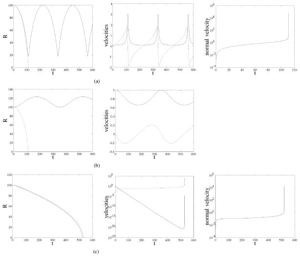
Fig. 5 shows the evolution of the radius, R, the tangential velocity α (if applicable), the normal velocity β for a small initial value of α, a larger initial value of α, and with added friction, respectively.

Fig. 5.

Left column: Evolution of the radius for the normal velocity evolution (dashed line) and the full velocity evolution (solid line). Middle column: Evolution of normal velocity (dashed line) and tangential velocity (solid line) for the full velocity approach. Right column: Evolution of normal velocity for the normal velocity evolution. (a) α₀ = 0.1, β₀ = 0, R₀ = 100, γ_α = 0, γ_β = 0. (b) α₀ = 1, β₀ = 0, R₀ = 100, γ_α = 0, γ_β = 0. (c) α₀ = 1, β₀ = 0, R₀ = 100, γ_α = 0.1, γ_β = 0.1.

Fig. 5(a) shows the results for α₀ = 0.1, β₀ = 0, R₀ = 100, γ_α = 0, γ_β = 0. We see that while in the normal evolution case the circle accelerates rapidly and disappears in finite time, this is not the case when we do not neglect the tangential velocity: Then the circle oscillates. It rotates faster if it becomes smaller and slower if it becomes larger. Due to the small initial tangential velocity the radius evolution is initially similar in both cases. The oscillation effect is more drastic with increased initial tangential velocity (α₀ = 1). This can be seen in Fig. 5(b). Fig. 5(c) shows the results with added friction (γ_α = γ_β = 0.1). Both circles disappear in finite time. The evolutions of the radius look similar in both cases. Due to the large friction coefficients a large amount of energy gets dissipated; oscillations no longer occur.

Equations (18) and (19) do not exhibit the same behavior. Depending on the initial value for α, they will have fundamentally different solutions. For $\alpha =\pm \sqrt{2/3}$, and β₀ = 0 in (19), the solution is (geometrically) stationary, and the circle will keep its shape and rotate with velocity α for all times. Also if α₀ = 0, in this example case, both evolutions will be identical.

VII. Level Set Formulation

There are different ways to implement the derived curve evolution equations (see, for example, [38]); many numerical schemes exist. In this paper, we will restrict ourselves to level set based curve representations. In contrast to the classical level set approach [65], where the curve evolution speed is usually based on geometric properties of the curve or induced by some external process, the level set approach developed in this paper attaches a velocity field to the curve and evolves it dynamically. We distinguish between full and partial level set implementations. In the full case, curves evolve in a space consistent with the dimensionality of the problem. Geometric dynamic curve evolution would thus be performed in ℝ⁴ in the simplest case (since we are looking at planar curves). The codimensionality will increase if additional information is to be attached to the curve. Normal geometric dynamic curve evolution would be at least a problem in ℝ³. If n is the dimensionality of the problem the curve can for example be implicitly described by the zero level set of an n-dimensional vector distance function or the intersection of n − 1 hypersurfaces [66]. Full level set approaches of this form are computationally expensive, since the evolutions are performed in high dimensional spaces. Furthermore, it is not obvious how to devise a methodology comparable to a narrow band scheme [67] in the case of a representation based on intersecting hypersurfaces.

A partial level set approach uses a level set formulation for the propagation of an implicit description of the curve itself (thus allowing for topological changes), but explicitly propagates the velocity information associated with every point on the contour by means of possibly multiple transport equations. This method has the advantage of computational efficiency (a narrow band implementation is possible in this case, and the evolution is performed in a low dimensional space) but sacrifices object separation: Tracked objects that collide will be merged.

In what follows, we will restrict ourselves to a partial level set implementation of the normal geometric dynamic curve evolution (i.e., α = 0 ∀s, t). We will investigate the full level set implementation, including tangential velocities, in our future work.

A. Partial Level Set Approach for the Normal Geometric Curve Evolution

The curve is represented as the zero level set of the function

$$\mathrm{\Phi }(\mathit{x}(t),t):{\mathbb{R}}^2\times {\mathbb{R}}^{+}\mapsto \mathbb{R}$$

where x(t) = (x(t), y(t))^T is a point in the image plane. We choose Φ to be a signed distance function, i.e., ||∇Φ|| = 1, a.e., such that Φ > 0 outside the curve and Φ < 0 inside the curve . Since the evolution of the curve’s shape is independent of the tangential velocity, we can write the level set evolution equation for an arbitrary velocity x_t as

$${\mathrm{\Phi }}_t-\left|\right|\nabla \mathrm{\Phi }\left|\right|\mathcal{N}·{\mathit{x}}_t=0$$ (20)

where

$$\mathcal{N}=-\frac{\nabla \mathrm{\Phi }}{\left|\right|\nabla \mathrm{\Phi }\left|\right|}.$$

In our case x_t = β̃ , where

$$\stackrel{\sim }{\beta }(\mathit{x},t)=\beta (p,t)$$ (21)

is the spatial normal velocity at the point x. This simplifies (20) to

$${\mathrm{\Phi }}_t-\stackrel{\sim }{\beta }\left|\right|\nabla \mathrm{\Phi }\left|\right|=0.$$ (22)

Substituting (21) into (16) and using the relation

$$\kappa =\nabla ·\left(\frac{\nabla \mathrm{\Phi }}{\left|\right|\nabla \mathrm{\Phi }\left|\right|}\right)$$

yields

$${\stackrel{\sim }{\beta }}_t=\stackrel{\sim }{\beta }\nabla \stackrel{\sim }{\beta }\frac{\nabla \mathrm{\Phi }}{\left|\right|\nabla \mathrm{\Phi }\left|\right|}=\left(\frac{1}{2}{\stackrel{\sim }{\beta }}^2+\frac{1}{\mu }g\right)\kappa +\frac{1}{\mu }\nabla g·\frac{\nabla \mathrm{\Phi }}{\left|\right|\nabla \mathrm{\Phi }\left|\right|}.$$ (23)

The left-hand side of (23) is the material derivative for the normal velocity. If we use extension velocities, (23) simplifies to

$${\stackrel{\sim }{\beta }}_t=\left(\frac{1}{2}{\stackrel{\sim }{\beta }}^2+\frac{1}{\mu }g\right)\kappa +\frac{1}{\mu }\nabla g·\frac{\nabla \mathrm{\Phi }}{\left|\right|\nabla \mathrm{\Phi }\left|\right|}.$$

Since the extensions are normal to the contours, normal propagation of the level set function will guarantee a constant velocity value along the propagation direction (up to numerical errors). Specifically ∇β̃⊥∇Φ in this case and thus

$$\nabla \mathrm{\Phi }·\nabla \stackrel{\sim }{\beta }=0.$$

For an alternative derivation,⁵ we change our Lagrangian, and extend it over a range of level sets. For each time t and 0 ≤ r ≤ 1, let

$${\mathcal{C}}^{(r)}(t):=\{(x,y)\in {\mathbb{R}}^2:\mathrm{\Phi }(x,y,t)=r\}.$$

Using the Lagrangian

$$L={\int }_0^1{\int }_{{\mathcal{C}}^{(r)}(t)}\left(\frac{1}{2}\mu {\stackrel{\sim }{\beta }}^2-g\right)dsdr$$

we obtain the action integral

$$\mathcal{L}={\int }_t{\int }_0^1{\int }_{{\mathcal{C}}^{(r)}(t)}\left(\frac{1}{2}\mu {\stackrel{\sim }{\beta }}^2-g\right)dsdrdt$$

which is

$$\begin{array}{l}\mathcal{L}={\int }_0^1{\int }_0^T{\int }_{{\mathcal{C}}^{(r)}(t)}\left(\frac{1}{2}\mu {\stackrel{\sim }{\beta }}^2-g\right)dsdtdr\\ ={\int }_0^T\left({\int }_0^1{\int }_{{\mathcal{C}}^{(r)}(t)}\left(\frac{1}{2}\mu {\stackrel{\sim }{\beta }}^2-g\right)d{\mathcal{H}}^1\lfloor {\mathcal{C}}^{(r)}(t)\rfloor dr\right)dt\\ ={\int }_0^T{\int }_{\mathrm{\Omega }}\left(\frac{1}{2}\mu {\stackrel{\sim }{\beta }}^2-g\right)\left|\right|\nabla \mathrm{\Phi }\left|\right|dxdydt\end{array}$$ (24)

where is the one-dimensional Hausdorff measure and we applied the coarea formula [68]. This casts the minimization problem into minimization over an interval of level sets in a fixed coordinate frame (x and y are time independent coordinates in the image plane). Using (22), we express β̃ as

$$\stackrel{\sim }{\beta }=\frac{{\mathrm{\Phi }}_t}{\left|\right|\nabla \mathrm{\Phi }\left|\right|}.$$ (25)

Substituting (25) into (24) yields

$$\mathcal{L}[\mathrm{\Phi }]:={\int }_0^T{\int }_{\mathrm{\Omega }}\left(\mu \frac{{\mathrm{\Phi }}_t^2}{2\left|\right|\nabla \mathrm{\Phi }\left|\right|}-g\left|\right|\nabla \mathrm{\Phi }\left|\right|\right)dxdydt$$

which is the new Φ-dependent action integral to be minimized. Then, δ = 0 if and only if

$$\frac{\partial }{\partial t}\left(\frac{{\mathrm{\Phi }}_t}{\left|\right|\nabla \mathrm{\Phi }\left|\right|}\right)=\nabla ·\left(\left(\frac{g}{\mu }+\frac{{\mathrm{\Phi }}_t^2}{{\left|\right|\nabla \mathrm{\Phi }\left|\right|}^2}\right)\frac{\nabla \mathrm{\Phi }}{\left|\right|\nabla \mathrm{\Phi }\left|\right|}\right).$$

The curve evolution is thus governed by the equation system

$$\begin{array}{l}{\stackrel{\sim }{\beta }}_t=\nabla ·\left(\frac{\nabla \mathrm{\Phi }}{\left|\right|\nabla \mathrm{\Phi }\left|\right|}\left(\frac{g}{\mu }+\frac{1}{2}{\stackrel{\sim }{\beta }}^2\right)\right)\\ {\mathrm{\Phi }}_t=\stackrel{\sim }{\beta }\left|\right|\nabla \mathrm{\Phi }\left|\right|.\end{array}$$ (26)

Expanding (26) yields again

$${\stackrel{\sim }{\beta }}_t=\left(\frac{1}{2}{\stackrel{\sim }{\beta }}^2+\frac{1}{\mu }g\right)\kappa +\frac{1}{\mu }\nabla g·\frac{\nabla \mathrm{\Phi }}{\left|\right|\nabla \mathrm{\Phi }\left|\right|}+\stackrel{\sim }{\beta }\nabla \stackrel{\sim }{\beta }·\frac{\nabla \mathrm{\Phi }}{\left|\right|\nabla \mathrm{\Phi }\left|\right|}.$$

The equation system (26) constitutes a conservation law for the normal velocity β̃. The propagation of the level set function Φ is described (as usual) by a Hamilton-Jacobi equation.

VIII. Error Injection

A system governed by a time-independent Lagrangian (i.e., L_t ≡ 0) will preserve energy [58], but this is not necessarily desirable. Indeed, envision a curve evolving on a static image with an initial condition of zero normal velocity everywhere and with an initial position of nonminimal potential energy. The curve will oscillate in its potential well indefinitely. One solution to this problem is to dissipate energy [33], which can be accomplished by simply adding a friction term to (26). However, to increase robustness it is desirable to be able to dissipate and to add energy to the system in a directed way. A principled way to do this would be to use an observer to drive the system state of the evolving curve to the object(s) to be tracked. In our case this is not straightforward, since we are dealing with an infinite dimensional nonlinear system. In order for the curve to approximate the dynamic behavior of the tracked objects we use error injection. This guarantees convergence of the curve to the desired object(s) if the curve is initially in the appropriate basin of attraction.

To perform error injection, we need an estimated position and velocity vector for every point on the curve . Define the line through the point x(s) on the current curve as

$$l(s,p):=\mathit{x}(s)-p\mathcal{N}$$

and the set of points in an interval (a, b) on the line as

$$L(a,b,s):=\{l(s,p),a<p<b)\}.$$

Define

$$\begin{array}{l}f(s):=inf\{p:p<0,\mathrm{\Phi }(\mathit{x})\le 0\forall \mathit{x}\in L(p,0,s)\}\\ t(s):=sup\{p:p>0,\mathrm{\Phi }(\mathit{x})\ge 0\forall \mathit{x}\in L(0,p,s)\}.\end{array}$$

Our set of estimated contour point candidates Z is the set of potential edge points in L(f, t, s)

$$\begin{array}{l}Z(L(f,t,s)):=\{\mathit{x}:\mathit{x}\in L(f,t,s),\exists \epsilon >0:\\ \left|\right|\nabla (G\ast I(\mathit{x}))\left|\right|>\left|\right|\nabla (G\ast I(\mathit{y}))\left|\right|\forall \mathit{y}\in L(f,t,s)\cap B_{\epsilon }(\mathit{x}),\mathit{y}\ne \mathit{x}\}\end{array}$$

where G is a Gaussian, B_ε(x) is the disk around x with radius ε, and I is the current image intensity. Given some problem specific likelihood function m(z) the selected contour point is the likelihood maximum

$${\mathit{x}}_c(s)=\underset{\mathit{z}\in Z(L(f,t,s))}{argmax}m(\mathit{z})$$

at position

$$p_c=d(\mathit{x},s)={(\mathit{x}(s)-{\mathit{x}}_c(s))}^T\mathcal{N}.$$

It is sufficient to estimate normal velocity, since the curve evolution equation does not take tangential velocity components into account. The estimation then can be performed (assuming we have brightness constancy from image frame to image frame for a moving image point) by means of the optical flow constraint without the need for regularization. Note that we compute this estimate only on a few chosen points in Z. The optical flow constraint is given as

$$I_t+{uI}_x+{vI}_y=0$$

where u = x_t and v = y_t are the velocities in the x and the y direction, respectively. We restrict the velocities to the normal direction by setting

$$\left(\begin{array}{c}u\\ v\end{array}\right)=\gamma \frac{\nabla I}{\left|\right|\nabla I\left|\right|}.$$

This yields

$$\gamma =-\frac{I_t}{\left|\right|\nabla I\left|\right|}$$

and thus the desired velocity estimate

$$\left(\begin{array}{c}u\\ v\end{array}\right)=-I_t\frac{\nabla I}{{\left|\right|\nabla I\left|\right|}^2}.$$

We define

$$\begin{array}{l}\overline{\beta }:=-\gamma \frac{\nabla I}{\left|\right|\nabla I\left|\right|}·\frac{\nabla \widehat{\mathrm{\Phi }}}{\left|\right|\nabla \widehat{\mathrm{\Phi }}\left|\right|}\\ \overline{\mathrm{\Phi }}:=-\left|\right|{\mathit{x}}_c-\mathit{x}\left|\right|\text{sign}\left(\widehat{\mathrm{\Phi }}({\mathit{x}}_c)\right).\end{array}$$

We propose using the following observer-like dynamical system:

$$\begin{array}{l}{\widehat{\mathrm{\Phi }}}_t=\left(m({\mathit{x}}_c)K_{\mathrm{\Phi }}(\overline{\mathrm{\Phi }}-\widehat{\mathrm{\Phi }})+\widehat{\beta }+\gamma \kappa \right)\left|\right|\nabla \widehat{\mathrm{\Phi }}\left|\right|\\ {\widehat{\beta }}_t=m({\mathit{x}}_c)K_{\beta }(\overline{\beta }-\widehat{\beta })+\left(\frac{1}{2}{\widehat{\beta }}^2+\frac{g}{\mu }\right)\kappa +\frac{1}{\mu }\nabla g·\frac{\nabla \widehat{\mathrm{\Phi }}}{\left|\right|\nabla \widehat{\mathrm{\Phi }}\left|\right|}+\delta {\widehat{\beta }}_{ss}\end{array}$$ (27)

to dynamically blend the current curve into the desired curve (see Fig. 7). Here, K_Φ and K_β are the error injection gains for Φ̂ and β̂, respectively. Any terms related to image features are computed at the current location x of the contour. The error injection gains are weighted by the likelihood m(x_c) of the correspondence points as a measure of prediction quality. The additional terms κγ and δβ̂_ss with tunable weighting factors γ and δ are introduced to allow for curve and velocity regularization if necessary, where

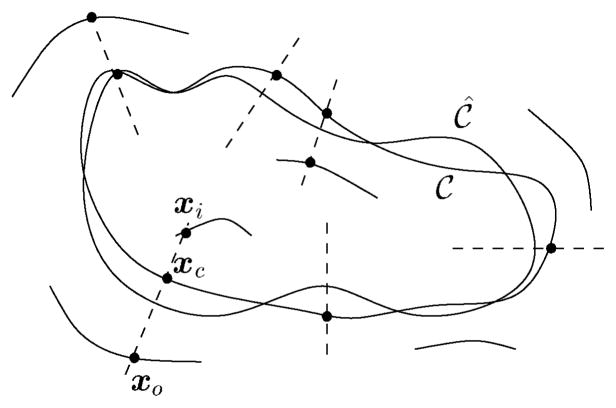
Fig. 7.

Correspondence point x_c, inside correspondence point x_i, and outside correspondence point x_o of the curve . represents the contour of the object to be tracked.

$$\begin{array}{l}\kappa =\nabla ·\left(\frac{\nabla \widehat{\mathrm{\Phi }}}{\left|\right|\nabla \widehat{\mathrm{\Phi }}\left|\right|}\right)\\ \text{and}{\widehat{\beta }}_{ss}={\mathcal{N}}^T\left(\begin{array}{cc}{\widehat{\beta }}_{yy}& -{\widehat{\beta }}_{xy}\\ -{\widehat{\beta }}_{xy}& {\widehat{\beta }}_{xx}\end{array}\right)\mathcal{N}+\kappa \nabla \widehat{\beta }·\mathcal{N}.\end{array}$$

In case no correspondence point for a point on the zero level set of Φ̂ is found, the evolution equation system (27) is replaced by

$$\begin{array}{l}{\widehat{\mathrm{\Phi }}}_t=(\beta +\gamma \kappa )\left|\right|\nabla \widehat{\mathrm{\Phi }}\left|\right|\\ {\widehat{\beta }}_t=\delta {\widehat{\beta }}_{ss}\end{array}$$ (28)

for this point.

IX. Computational Complexity of the Algorithm

Level set methods increase the computational complexity of curve evolution approaches. In the planar case, a one-dimensional curve is represented as the zero level set of a function defined on the two-dimensional image plane, Ω. Level set methods are of interest numerically (e.g., there is no fixed number of particles to represent a curve and topological changes are handled naturally), however, the evolution of the level set function far away from the zero level set is in general irrelevant and increases the computational complexity without providing additional benefits. Thus, instead of updating a level set evolution equation over all of Ω (which incurs an update cost of (n²), if Ω is represented on a square domain with n² discrete gridpoints) the computational domain Ω_c is chosen to be a band surrounding the zero level set up to a certain distance. This is the idea of the narrowband method [69]. If the narrowband consists of N points, the computational complexity consequently reduces from (n²) to (N). Frequently, the speed function β̂ is only defined or sensible on or very close to the zero level set and needs to be extended to the whole computational domain. This may be accomplished for example by the fast marching method [70], [65], [71] with a computational complexity of (N log N) or with a fast sweeping method [72] with a computational complexity of (N). The latter is extremely efficient for many “simple” flow fields (i.e., flow fields that are spatially regular and do not change direction frequently) that are encountered in practice (e.g., normal extensions as employed in this paper), but may require a relatively large number of iterations for flow fields that (for an individual particle stream line) fluctuate in direction.

For a narrowband implementation (with N points) of the tracking algorithm proposed in Section VIII the computational complexity is thus (N) for every evolution step of

$${\widehat{\mathrm{\Phi }}}_t=\left(m({\mathit{x}}_c)K_{\mathrm{\Phi }}(\overline{\mathrm{\Phi }}-\widehat{\mathrm{\Phi }})+\widehat{\beta }+\gamma \kappa \right)\left|\right|\nabla \mathrm{\Phi }\left|\right|$$

which includes the search for the feature points to determine Φ̄. Reinitialization of Φ̂ (which has to be performed relatively infrequently if extension velocities for β̂ are used) is of (N) or (N log N) (for a fast sweeping scheme and fast marching, respectively). The evolution of

$${\widehat{\beta }}_t=m({\mathit{x}}_c)K_{\beta }(\overline{\beta }-\widehat{\beta })+\left(\frac{1}{2}{\widehat{\beta }}^2+\frac{g}{\mu }\right)\kappa +\frac{1}{\mu }\nabla g·\frac{\nabla \widehat{\mathrm{\Phi }}}{\left|\right|\nabla \widehat{\mathrm{\Phi }}\left|\right|}+\delta {\widehat{\beta }}_{ss}$$

is again of complexity (N) for every evolution step, (N) or (N log N) for the velocity extension, and (N) to find the feature points β̄;. The computational complexity to find the values for a feature point Φ̄ and β̄ is constant, scales with the length of the line segment the search is performed over, but gets multiplied by the number of points in the narrowband N. The overall computational complexity of the algorithm is thus (N) when using a fast sweeping method or (N log N) for the fast marching method. Only the redistancing and the computation of the extension velocities cannot be easily parallelized. The proposed algorithm is in principle of the same order of computational complexity as the standard geodesic active contour (though admittedly with a larger computational cost per point, especially if the feature point search is not parallelized) for which real time implementations at standard camera frame rates exist.

X. Occlusion Detection

An occlusion in the context of this paper is any image change that renders the object to be tracked partially (partial occlusion) or completely (full occlusion) unobservable, e.g., when an object moves in between the camera and the object to be tracked and thus covers up parts or all of the latter. Tracking algorithms need to utilize shape information and/or (at least for short-time partial occlusions) make use of the time history of the object being tracked (i.e., its dynamics) to be able to tolerate occlusions. Static segmentation methods that do not use shape information will in general not be able to handle occlusions.

This section introduces a simple occlusion detection algorithm⁶ based on ideas in [73] to be used in conjunction with the dynamic tracking algorithm proposed in Section VIII to handle short-time partial occlusions.

The inside and the outside correspondence points are defined as (see Fig. 7)

$${\mathit{x}}_i(s)=\underset{\mathit{z}\in Z(L(f,p_c,s))}{argmax}m(\mathit{z}),{\mathit{x}}_o(s)=\underset{\mathit{z}\in Z(L(p_c,t,s)).}{argmax}m(\mathit{z}).$$

The occlusion detection strategy is split into the following six subcases for every point on the contour.

1. There is no correspondence point.

2. Only the correspondence point is present.

3. The point is moving outward, the correspondence point is present, but not its outside correspondence point.

4. The point is moving inward, the correspondence point is present, but not its inside correspondence point.

5. The point is moving outward, both the correspondence point and its outside correspondence point are present.

6. The point is moving inward, both the correspondence point and its inside correspondence point are present.

We define the following Gaussian conditional probabilities:

$$\begin{array}{c}Pr(t_{\mathit{occ}}\mid \mathit{occ})=\frac{1}{\sqrt{2\pi }{\sigma }_t}{e}^{-{(t_{\mathit{occ}}-{\mu }_t)}^2/2{\sigma }_t^2}\\ Pr(v_a\mid \mathit{occ})=\frac{1}{\sqrt{2\pi }{\sigma }_v}{e}^{-{(v_a-{\mu }_v)}^2/2{\sigma }_v^2}\\ Pr(t_{\mathit{occ}}\mid \overline{\mathit{occ}})=\frac{1}{\sqrt{2\pi }{\sigma }_{\overline{t}}}{e}^{-{(t_{\mathit{occ}}-{\mu }_{\overline{t}})}^2/2{\sigma }_{\overline{t}}^2}\\ Pr(v_a\mid \overline{\mathit{occ}})=\frac{1}{\sqrt{2\pi }{\sigma }_{\overline{v}}}{e}^{-{(v_a-{\mu }_{\overline{v}})}^2/2\sigma \frac{2}{v}}\end{array}$$

where t_occ is the estimated time to occlusion, v_a is the velocity of the point ahead, overlined symbols denote negated values (i.e., $\overline{\mathit{occ}}$ means not occluded), Pr(t_occ|occ), Pr(v_a|occ) are the probabilities of t_occ and v_a given an occlusion, and $Pr(t_{\mathit{occ}}\mid \overline{\mathit{occ}})$ and $Pr(v_a\mid \overline{\mathit{occ}})$ given there is no occlusion, respectively. The corresponding standard deviations are σ_t, σ_v, σ_t̄, and σ_v̄; the means are μ_t, μ_v, μ_t̄, μ_v̄. To compute the values of t_occ and v_a we make use of the currently detected correspondence point x_c, and its interior x_i and exterior x_o correspondence points.

The probability for an occlusion is given by Bayes’ formula as

$$Pr(\mathit{occ}\mid v_a,t_{\mathit{occ}})=\frac{Pr(v_a,t_{\mathit{occ}}\mid \mathit{occ})Pr(\mathit{occ})}{Pr(v_a,t_{\mathit{occ}}\mid \mathit{occ})Pr(\mathit{occ})+Pr(v_a,t_{\mathit{occ}}\mid \overline{\mathit{occ}})Pr(\overline{\mathit{occ}})}.$$

We initialize Pr(occ) = 0 and $Pr(\overline{\mathit{occ}})=1$ everywhere. The priors at time step n +1 are the smoothed posteriors of time step n. In case 0), Pr(occ|v_a, t_occ) = Pr(occ) (i.e., the probability is left unchanged), in all other cases

$$\begin{array}{l}Pr(\mathit{occ}\mid v_a\mid t_{\mathit{occ}})=\frac{{Pr}_{\mathit{occ}}^{i}Pr(\mathit{occ})}{{Pr}_{\mathit{occ}}^{i}Pr(\mathit{occ})+{Pr}_{\overline{\mathit{occ}}}^{i}Pr(\overline{\mathit{occ}})}\\ \text{where}{Pr}_{\mathit{occ}}^1=Pr(v_a=v_c\mid \mathit{occ})\\ {Pr}_{\overline{\mathit{occ}}}^1=Pr(v_a=v_c\mid \overline{\mathit{occ}})\\ {Pr}_{\mathit{occ}}^2=\{\begin{array}{ll}Pr(v_a=v_c\mid \mathit{occ}),\hfill & \text{if}{\mathit{x}}_c\text{outside}of\mathcal{C}\hfill \\ 0,\hfill & \text{otherwise}\hfill \end{array}\\ {Pr}_{\overline{\mathit{occ}}}^2=\{\begin{array}{ll}Pr(v_a=v_c\mid \overline{\mathit{occ}}),\hfill & \text{if}{\mathit{x}}_c\text{outside}of\mathcal{C}\hfill \\ 0,\hfill & \text{otherwise}\hfill \end{array}\\ {Pr}_{\mathit{occ}}^3=\{\begin{array}{ll}Pr(v_a=v_c\mid \mathit{occ}),\hfill & \text{if}{\mathit{x}}_c\text{inside}of\mathcal{C}\hfill \\ 0,\hfill & \text{otherwise}\hfill \end{array}\\ {Pr}_{\overline{\mathit{occ}}}^3=\{\begin{array}{ll}Pr(v_a=v_c\mid \overline{\mathit{occ}}),\hfill & \text{if}{\mathit{x}}_c\text{inside}of\mathcal{C}\hfill \\ 0,\hfill & \text{otherwise}\hfill \end{array}\\ {Pr}_{\mathit{occ}}^4=Pr(v_a=v_o\mid \mathit{occ})Pr(t_{\mathit{occ}}=t_{\mathit{occ}}^o\mid \mathit{occ})\\ {Pr}_{\overline{\mathit{occ}}}^4=Pr(v_a=v_o\mid \overline{\mathit{occ}}Pr(t_{\mathit{occ}}=t_{\mathit{occ}}^o\mid \overline{\mathit{occ}})\\ {Pr}_{\mathit{occ}}^5=Pr(v_a=v_i\mid \mathit{occ})Pr(t_{\mathit{occ}}=t_{\mathit{occ}}^i\mid \mathit{occ})\\ {Pr}_{\overline{\mathit{occ}}}^5=Pr(v_a=v_i\mid \overline{\mathit{occ}})Pr(t_{\mathit{occ}}=t_{\mathit{occ}}^i\mid \overline{\mathit{occ}})\\ \text{and}{v}_c=\overline{\beta }({\mathit{x}}_c)v_o=\overline{\beta }({\mathit{x}}_o)\\ v_i=\overline{\beta }({\mathit{x}}_i)v=\overline{\beta }(\mathit{x})\\ t_{\mathit{occ}}^i=\frac{\left|\right|\mathit{x}-x_i\left|\right|}{\mid v-v_i\mid }{t}_{\mathit{occ}}^o=\frac{\left|\right|\mathit{x}-{\mathit{x}}_o\left|\right|}{\mid v-v_o\mid }.\end{array}$$

To estimate the current rigid body motion, the following system:

$$\begin{array}{l}{(u_r,v_r)}^T{\int }_{\mathcal{C}}{n}^1\mathcal{N}ds=-{\int }_{\mathcal{C}}{n}^1\beta ds\\ {(u_r,v_r)}^T{\int }_{\mathcal{C}}{n}^2\mathcal{N}ds=-{\int }_{\mathcal{C}}{n}^2\beta ds\end{array}$$

is solved, where = (n¹, n²)^T. We set μ_v̄ = −(u_r, v_r)^T and μ_v = 0.

The evolution equation is changed to

$$\begin{array}{l}{\widehat{\mathrm{\Phi }}}_t=\left(Pr(\overline{\mathit{occ}})\left(m({\mathit{x}}_c)K_{\mathrm{\Phi }}(\overline{\mathrm{\Phi }}-\widehat{\mathrm{\Phi }})\right)+\widehat{\beta }+\gamma \kappa \right)\left|\right|\nabla \widehat{\mathrm{\Phi }}\left|\right|\\ {\widehat{\beta }}_t=Pr(\overline{\mathit{occ}})\left(m({\mathit{x}}_c)K_{\beta }(\overline{\beta }-\widehat{\beta })+\left(\frac{1}{2}{\widehat{\beta }}^2+\frac{g}{\mu }\right)\kappa \right)+Pr(\overline{\mathit{occ}})\frac{1}{\mu }\nabla g\kappa +\delta {\widehat{\beta }}_{ss}.\end{array}$$

This is an interpolation between (27) and (28) based on the occlusion probability.

XI. Simulation Results

The proposed tracking algorithm is tested on two real video sequences. Fig. 9 shows three frames of a fish sequence and Fig. 10 shows three frames of a car sequence. In both cases occlusions occur. For the fish sequence no occlusion detection is performed, to demonstrate the behavior of the normal geometric curve evolution algorithm alone, on an image sequence with a short-time partial occlusion. Define⁷

Fig. 9.

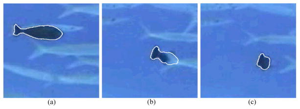
Three frames of a fish sequence. This is a color image. (a) Frame 0. (b) Frame 80. (c) Frame 90. (Color version available online at http://ieeexplore.ieee.org.)

Fig. 10.

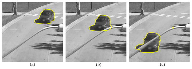
Three frames of a car sequence. This is a color image. (a) Frame 0. (b) Frame 14. (c) Frame 55. (Color version available online at http://ieeexplore.ieee.org.)

$$\begin{array}{l}q(x):=\frac{1}{1+e^{-(p_1+x)}}r:=q(0)+\frac{e^{-p_1}}{q{(0)}^2}{p}_2\\ w(\mathit{x}):=\{\begin{array}{ll}q(d(\mathit{x})),\hfill & \text{if}d(\mathit{x})\le 0\hfill \\ q(0)+\frac{e^{-p_1}}{q{(0)}^2}d(\mathit{x}),\hfill & \text{if}0<d(\mathit{x})\le p_2\hfill \\ r-\frac{r}{p_3-p_2}(d(\mathit{x})-p_2),\hfill & \text{if}{p}_2<d(\mathit{x})\le p_3\hfill \\ 0,\hfill & \text{otherwise}.\hfill \end{array}\end{array}$$

The used likelihood function for the fish sequence is

$$m(\mathit{z})=e^{-\left({(g(\mathit{z})-{\mu }_g)}^2/2{\sigma }_g^2+{(I(\mathit{z})-{\mu }_I)}^2/2{\sigma }_I^2\right)}w(\mathit{z}).$$

The function depends on the image intensity I, the potential function g, and the distance d to the contour.

For the car sequence, we define

$$\begin{array}{l}a(\mathit{x}):=arccos\left(\frac{\nabla (G\ast I)}{\left|\right|\nabla (G\ast I)\left|\right|}·\mathcal{N}\right)\\ a_n(\mathit{x}):=min(\mid a(\mathit{x})\mid ,\pi -\mid a(\mathit{x})\mid ).\end{array}$$

This is a measure of angle difference between edge orientation at correspondence points and the normal of the curve. Ideally, both should be aligned. The likelihood for a contour point candidate z ∈ Z is then computed as

$$m(\mathit{z})=e^{-\left({(\mid d(\mathit{z})\mid -{\mu }_d)}^2/2{\sigma }_d^2+{(g(\mathit{z})-{\mu }_g)}^2/2{\sigma }_g^2+{(a_n(\mathit{z})-{\mu }_a)}^2/2{\sigma }_a^2\right)}$$

and the occlusion detection of Section X is performed.

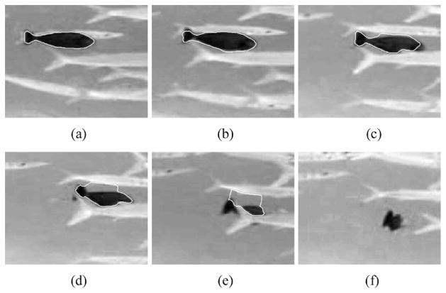
In both cases occlusions are handled. For the fish sequence the occlusion is dealt with implicitly. The occluding fish moves over the tracked fish quickly, so that the inertia effects keep the fish at a reasonable location. For comparison Fig. 11 shows the tracking of the fish in six frames of the same fish sequence by means of a geodesic active contour. Here, the motion model is static (i.e., the converged to location at frame n is the initial condition for the curve evolution at frame n+1) and the tracking result at every frame represents the steady state of the geodesic active contour evolution (6). While the fish is tracked initially, the tracking contour subsequently adheres to a second fish and finally looses track completely.

Fig. 11.

Six frames of a fish sequence. Tracking using the geodesic active contour. (a) Frame 0. (b) Frame 30. (c) Frame 45. (d) Frame 60. (e) Frame 75. (f) Frame 90.

For the car example the occlusion (the lamp post) is treated explicitly by means of the proposed occlusion detection algorithm. In both cases the likelihood functions do not incorporate any type of prior movement information. Doing so would increase robustness, but limit flexibility. Finally, since this active contour model is edge-based, the dynamic active contour captures the sharp edge of the shadow in the car sequence. Presumably this could be handled by including more global area-based terms or shape information in the model.

XII. Conclusion and Future Work

In this paper, we proposed a new approach for visual tracking based on dynamic geodesic active contours. This methodology incorporates state information (here, normal velocity, but any other kind of state information can be treated in a similar way) with every particle on a contour described by means of a level set function. It has the potential to deal with partial occlusions.

Edge-based approaches trade off robustness for versatility. If strong, clear edge information exists they are a very useful class of algorithms; however, in many cases more robust techniques are required. Methods that incorporate area-based influence terms have proven to be very efficient for certain applications. To add more robustness to our methodology, we are currently working on a dynamic area based approach based on elasticity theory.

Our proposed algorithm searches for image features (i.e., likelihood maxima) along normal lines of an evolving contour. Thus, the algorithm lies between purely edge-based and purely area-based approaches. This ties in very well with the proposed occlusion detection algorithm, but it places much importance in finding the “correct” correspondence points. The main disadvantage of the occlusion detection algorithm is the large number of tunable parameters it requires. Devising a less parametric occlusion algorithm would be beneficial.

We also do not claim that our algorithm is optimal for the specific image sequences presented. Indeed, whenever possible, additional information should be introduced. If we know we want to track a car, we should make use of the shape information we have. Not all deformations will make sense in this case. Our main contribution lies in putting dynamic curve evolution into a geometric framework and in demonstrating that we can transport any kind of information along with a curve (e.g., marker particles, enabling us to follow the movement of specific curve parts over time). This gives us increased flexibility and enables fundamentally different curve behaviors than in the static (non-informed) case often used in the computer vision community. Furthermore, applications for dynamic geodesic active contours need not be restricted to tracking, e.g., applications in computer graphics are conceivable (where the curve movement would then be physically motivated), not necessarily involving an underlying real image (e.g., we could design artificial potential fields enforcing a desired type of movement).

As geodesic active contours extend to geodesic active surfaces, dynamic geodesic active contours can be extended to dynamic geodesic surfaces. Our main focus for future research will be an extension toward area based dynamic evolutions.

Fig. 6.

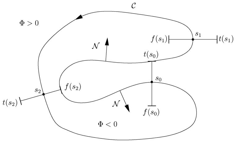
Feature search is performed in the normal direction to the curve. The search region is only allowed to intersect the curve at its origin of search (i.e., s₀, s₁, s₂, …).

Fig. 8.

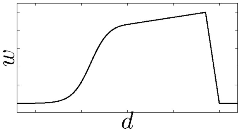
Illustration of the shape of the weighting function w(x) for the fish sequence.

Biographies

Marc Niethammer received the Dipl.-Ing. in engineering cybernetics from the Universität Stuttgart, Stuttgart, Germany, in 2000, and the M.S. degree in engineering science and mechanics, the M.S. degree in applied mathematics, and the Ph.D. degree in electrical and computer engineering, all from the Georgia Institute of Technology, Atlanta, in 1999, 2002, and 2004, respectively.

He is currently a Research Fellow at the Psychiatry Neuroimaging Lab, Brigham and Women’s Hospital, Harvard Medical School, Cambridge, MA.

Allen Tannenbaum received the Ph.D. degree in mathematics from Harvard University, Cambridge, MA, in 1976.

He is a faculty member at the Georgia Institute of Technology, Atlanta. His research interests are in control theory, image processing, and computer vision.

Sigurd B. Angenent received the Ph.D. degree in mathematics from the University of Leiden, Leiden, The Netherlands, in 1986.

He spent one year at the California Institute of Technology, Pasadena, on a NATO fellowship. He is currently a Professor of mathematics at the University of Wisconsin, Madison. His interests center on nonlinear partial differential equations in differential geometry. He is also interested in exploring the vast interface between pure mathematics, engineering, and the sciences.

Appendix I. Geometric Dynamic Curve Evolution

Equation (11) is derived as follows: assume the curve gets perturbed by ε yielding the curve

$${\mathcal{C}}^p=\mathcal{C}+\epsilon \mathcal{V}.$$

The action integral (7) becomes

$$\mathcal{L}(\mathcal{C}+\epsilon \mathcal{V})={\int }_{t=t_0}^{t_1}{\int }_{p=0}^1\left(\frac{1}{2}\mu {\left|\right|{\mathcal{C}}_t+\epsilon {\mathcal{V}}_t\left|\right|}^2-g(\mathcal{C}+\epsilon \mathcal{V})\right)\left|\right|{\mathcal{C}}_p+\epsilon {\mathcal{V}}_p\left|\right|dpdt.$$

$$\delta \mathcal{L}(\mathcal{C};\mathcal{V})={\frac{\partial \mathcal{L}}{\partial \epsilon }|}_{\epsilon =0}={\int }_{t=t_0}^{t_1}{\int }_{p=0}^1(\mu {\mathcal{C}}_t·{\mathcal{V}}_t-\nabla g·\mathcal{V})\left|\right|C_p\left|\right|+\left(\frac{1}{2}\mu {\left|\right|{\mathcal{C}}_t\left|\right|}^2-g\right)\frac{1}{\left|\right|{\mathcal{C}}_p\left|\right|}{\mathcal{C}}_p·{\mathcal{V}}_{p}dpdt.$$

$$\delta \mathcal{L}(\mathcal{C};\mathcal{V})={\int }_{t=t_0}^{t_1}{\int }_{p=0}^1-\frac{\partial }{\partial p}\left(\left(\frac{1}{2}\mu {\left|\right|{\mathcal{C}}_t\left|\right|}^2-g\right)\mathcal{T}\right)·\mathcal{V}\frac{1}{\left|\right|{\mathcal{C}}_p\left|\right|}\left|\right|{\mathcal{C}}_p\left|\right|-\nabla g·\mathcal{V}\left|\right|{\mathcal{C}}_p\left|\right|-\frac{\partial }{\partial t}(|\left|{\mathcal{C}}_p\right||\mu {\mathcal{C}}_t)·\mathcal{V}\frac{1}{\left|\right|{\mathcal{C}}_p\left|\right|}\left|\right|{\mathcal{C}}_p\left|\right|dpdt$$ (29)

We compute the Gâteaux variation by taking the derivative with respect to ε for ε = 0; see the first equation shown at the bottom of the page. Assuming μ to be constant integration by parts yields (29), as shown at the bottom of the page. The boundary terms occurring from the integrations by parts drop out for closed curves. Then, (since (29) has to be fulfilled for any )

$$\frac{\partial }{\partial s}\left(\left(\frac{1}{2}\mu {\left|\right|{\mathcal{C}}_t\left|\right|}^2-g\right)\mathcal{T}\right)+\nabla g+\frac{\partial }{\partial t}(|\left|{\mathcal{C}}_p\right||\mu {\mathcal{C}}_t)\frac{1}{\left|\right|{\mathcal{C}}_p\left|\right|}=0$$ (30)

where

$$\frac{\partial }{\partial s}=\frac{1}{\left|\right|{\mathcal{C}}_p\left|\right|}\frac{\partial }{\partial p}.$$

To simplify (30), we use the following correspondences:

$$\begin{array}{l}{\mathcal{C}}_{pt}={\mathcal{C}}_{tp}\\ \frac{1}{\left|\right|{\mathcal{C}}_p\left|\right|}\frac{\partial }{\partial t}\left|\right|{\mathcal{C}}_p\left|\right|=\frac{1}{2{\left|\right|{\mathcal{C}}_p\left|\right|}^2}2{\mathcal{C}}_p·{\mathcal{C}}_{pt}={\mathcal{C}}_s·{\mathcal{C}}_{ts}=\mathcal{T}·{\mathcal{C}}_{ts}\\ \frac{\partial }{\partial s}\mathcal{T}=\kappa \mathcal{N}\\ \frac{\partial }{\partial s}{\left|\right|{\mathcal{C}}_t\left|\right|}^2=\frac{1}{\left|\right|{\mathcal{C}}_p\left|\right|}\frac{\partial }{\partial p}({\left|\right|{\mathcal{C}}_t\left|\right|}^2)=\frac{1}{\left|\right|{\mathcal{C}}_p\left|\right|}2{\mathcal{C}}_t·{\mathcal{C}}_{tp}=2{\mathcal{C}}_t·{\mathcal{C}}_{ts}\\ \frac{\partial }{\partial s}g=\nabla g·\mathcal{T}\\ \frac{\partial }{\partial t}{\mathcal{C}}_t={\mathcal{C}}_{tt}.\end{array}$$

Specifically, it follows that

$$\begin{array}{l}\frac{\partial }{\partial s}\left(\frac{1}{2}\mu {\left|\right|{\mathcal{C}}_t\left|\right|}^2-g\right)=\mu {\mathcal{C}}_t·{\mathcal{C}}_{ts}-\nabla g·\mathcal{T}\\ \frac{1}{\left|\right|{\mathcal{C}}_p\left|\right|}\frac{\partial }{\partial t}(|\left|{\mathcal{C}}_p\right||\mu {\mathcal{C}}_t)=\mu {\mathcal{C}}_{tt}+\mu (\mathcal{T}·{\mathcal{C}}_{ts}){\mathcal{C}}_t.\end{array}$$

Plugging everything in (30) results in

$$\mu {\mathcal{C}}_{tt}+\left(\frac{1}{2}\mu {\left|\right|{\mathcal{C}}_t\left|\right|}^2-g\right)\kappa \mathcal{N}+\frac{\partial }{\partial s}\left(\frac{1}{2}\mu {\left|\right|{\mathcal{C}}_t\left|\right|}^2-g\right)\mathcal{T}+\mu (\mathcal{T}·{\mathcal{C}}_{ts}){\mathcal{C}}_t+\nabla g=0$$ (31)

which is (11).

Appendix II. Coupled Normal and Tangential Evolution

The general version of the geometric dynamic curve evolution equation is given in (31) where is the unit inward normal and

$${\mathcal{T}}_s=\kappa \mathcal{N}{\mathcal{N}}_s=-\kappa \mathcal{T}.$$

We can always write

$${\mathcal{C}}_t=\alpha (p,t)\mathcal{T}+\beta (p,t)\mathcal{N}.$$

We choose the parameterization p such that it is independent of time. The parameterization thus travels with its particle.

Let us derive the general (without prespecified special reparameterization φ) evolution equations for α and β (see [64] for details on some of the equations used). Using an arbitrary curve parameterization p (with (p, 0) = (p, 1), = (p, t), and p ∈ [0, 1]) define

$$G(p,t):=\left|\right|{\mathcal{C}}_p\left|\right|={(x_p^2+y_p^2)}^{1/2}.$$

Arclength is then given by

$$s(p,t):={\int }_0^{p}G(\xi ,t)d\xi .$$

Then

$$\frac{\partial }{\partial t}\frac{\partial }{\partial s}=-\frac{1}{G}({\alpha }_p-\beta \kappa G)\frac{\partial }{\partial s}+\frac{\partial }{\partial s}\frac{\partial }{\partial t}.$$

We can also compute

$$G_t={\alpha }_p-\beta \kappa G.$$

From the previous expressions follows:

$${\mathcal{N}}_t=-({\beta }_s+\alpha \kappa )\mathcal{T}\text{and}{\mathcal{T}}_t=({\beta }_s+\alpha \kappa )\mathcal{N}.$$

This yields

$$\begin{array}{l}{\mathcal{C}}_{tt}={({\mathcal{C}}_t)}_t={(\alpha \mathcal{T}+\beta \mathcal{N})}_t\\ ={\alpha }_t\mathcal{T}+\alpha ({\beta }_s+\alpha \kappa )\mathcal{N}+{\beta }_t\mathcal{N}-\beta ({\beta }_s+\alpha \kappa )\mathcal{T}\\ =({\alpha }_t-\beta {\beta }_s-\alpha \beta \kappa )\mathcal{T}+(\alpha {\beta }_s+{\alpha }^2\kappa +{\beta }_t)\mathcal{N}\\ \text{and}{\mathcal{C}}_{ts}={(\alpha \mathcal{T}+\beta \mathcal{N})}_s\\ ={\alpha }_s\mathcal{T}+\alpha \kappa \mathcal{N}+{\beta }_s\mathcal{N}-\beta \kappa \mathcal{T}\\ =({\alpha }_s-\beta \kappa )\mathcal{T}+(\alpha \kappa +{\beta }_s)\mathcal{N}.\end{array}$$

Some simple algebra results in

$$\mu \left[({\alpha }_t-2\alpha \beta \kappa +2\alpha {\alpha }_s)\mathcal{T}+\left(\frac{3}{2}\kappa {\alpha }^2-\frac{1}{2}\kappa {\beta }^2+{\alpha }_s\beta +\alpha {\beta }_s+{\beta }_t\right)\mathcal{N}\right]=g\kappa \mathcal{N}-(\nabla g·\mathcal{N})\mathcal{N}$$

from (31), which can be written as

$$\mu [({\alpha }_t+2\alpha {\alpha }_s)\mathcal{T}+({\alpha }_s\beta +\alpha {\beta }_s+{\beta }_t)\mathcal{N}]=\left(2\alpha \beta \mu \mathcal{T}+\left(\frac{1}{2}{\beta }^2-\frac{3}{2}{\alpha }^2\right)\mu \mathcal{N}+g\mathcal{N}\right)\kappa -(\nabla g·\mathcal{N})\mathcal{N}.$$

With

$$\mathcal{T}=\left(\begin{array}{cc}0& -1\\ 1& 0\end{array}\right)\mathcal{N}$$

it follows that

$$\mu \left(\begin{array}{cc}{\alpha }_s\beta +\alpha {\beta }_s+{\beta }_t& -{\alpha }_t-2\alpha {\alpha }_s\\ {\alpha }_t+2\alpha {\alpha }_s& {\alpha }_s\beta +\alpha {\beta }_s+{\beta }_t\end{array}\right)\mathcal{N}=\mu \kappa \left(\begin{array}{cc}\left(\frac{1}{2}{\beta }^2-\frac{3}{2}{\alpha }^2\right)+\frac{1}{\mu }g& -2\alpha \beta \\ 2\alpha \beta & \left(\frac{1}{2}{\beta }^2-\frac{3}{2}{\alpha }^2\right)+\frac{1}{\mu }g\end{array}\right)\mathcal{N}-\mu \left(\begin{array}{cc}\frac{1}{\mu }\nabla g·\mathcal{N}& 0\\ 0& \frac{1}{\mu }\nabla g·\mathcal{N}\end{array}\right)\mathcal{N}.$$ (32)

This must be true for all . Equation (32) reduces to the following two coupled partial differential equations:

$$\begin{array}{l}{\alpha }_t=-{({\alpha }^2)}_s+2\kappa \alpha \beta \\ {\beta }_t=-{(\alpha \beta )}_s+\left[\left(\frac{1}{2}{\beta }^2-\frac{3}{2}{\alpha }^2\right)+\frac{1}{\mu }g\right]\kappa -\frac{1}{\mu }\nabla g·\mathcal{N}.\end{array}$$ (33)

References

- 1.Welch G, Foxlin E. Motion tracking: No silver bullet, but a respectable arsenal. IEEE Comput Graph Appl. 2002;22(6):24–38. [Google Scholar]
- 2.Julier S, Bishop G. Tracking: How hard can it be? IEEE Comput Graph Appl. 2002;22(6):22–23. [Google Scholar]
- 3.Allen BD, Bishop G, Welch G. Course Notes, Annu Conf Computer Graphics and Interactive Techniques (Siggraph 2001) 2001. Tracking: Beyond 15 minutes of thought: Siggraph 2001 course 11. [Google Scholar]
- 4.Ulmer B. VITA II – Active collision avoidance in real traffic. Proc Intelligent Vehicles Symp. 1994:1–6. [Google Scholar]
- 5.Malik J, Russell S. Tech Rep UCB-ITS-PRR-95-6. Univ. California; Berkeley: 1995. A machine vision based surveillance system for California Roads. [Google Scholar]
- 6.Beymer D, McLauchlan P, Coifman B, Malik J. A real-time computer vision system for measuring traffic parameters. Proc Conf Computer Vision and Pattern Recognition. 1997:495–501. [Google Scholar]
- 7.Franke U, Gavrila D, Görzig S, Lindner F, Paetzold F, Wöhler C. Autonomous driving goes downtown. IEEE Intell Syst. 1999;13(6):40–48. [Google Scholar]
- 8.Dickmanns ED. The 4D-approach to dynamic machine vision. Proc 33rd Conf Decision and Control. 1994:3770–3775. [Google Scholar]
- 9.McLauchlan PF, Malik J. Vision for longitudinal vehicle control. Proc Conf Intelligent Transportation Systems. 1997:918–923. [Google Scholar]
- 10.Sinopoli B, Micheli M, Donato G, Koo TJ. Vision based navigation for an unmanned aerial vehicle. Proc Int Conf Robotics and Automation. 2001:1757–1764. [Google Scholar]
- 11.Sharp CS, Shakernia O, Sastry SS. A vision system for landing an unmanned aerial vehicle. Proc Int Conf Robotics and Automation. 2001:1720–1727. [Google Scholar]
- 12.Remagnino P, Jones GA, Paragios N, Regazzoni CS, editors. Video-Based Surveillance Systems. Kluwer Academic; Norwell, MA: 2001. [Google Scholar]
- 13.Tanawongsuwan R, Bobick A. Gait recognition from time-normalized joint-angle trajectories in the walking plane. Proc Conf Computer Vision and Pattern Recognition. 2001;2:726–731. [Google Scholar]
- 14.Bhanu B, Dudgeon DE, Zelnio EG, Rosenfeld A, Casasent D, Reed IS. Introduction to the special issue on automatic target detection and recognition. IEEE Trans Image Process. 1997 Jan;6(1):1–6. [Google Scholar]
- 15.Corke P. Visual Servoing. Vol. 7. Singapore: World Scientific; Robotics and Automated Systems; 1993. Visual control of robotic manipulators – A review; pp. 1–31. [Google Scholar]
- 16.Hutchinson S, Hager GD, Corke PI. A tutorial on visual servo control. IEEE Trans Robot Automat. 1996 Oct;12(5):651–670. [Google Scholar]
- 17.Oka K, Sato Y, Koike H. Real-time fingertip tracking and gesture recognition. IEEE Comput Graph Appl. 2002;22(6):64–71. [Google Scholar]
- 18.Kansy K, Berlage T, Schmitgen G, Wiskirchen P. Real-time integration of synthetic computer graphics into live video scenes. Proc Conf Interface of Real and Virtual Worlds. 1995:93–101. [Google Scholar]
- 19.Hotraphinyo LF, Riviere CN. Precision measurement for microsurgical instrument evaluation. Proc 23rd Annu EMBS Int Conf. 2001:3454–3457. [Google Scholar]
- 20.Ayache N, Cohen I, Herlin I. Active Vision. Cambridge, MA: MIT Press; 1992. Medical image tracking; pp. 3–20. [Google Scholar]
- 21.Blake A, Yuille A, editors. Active Vision. MIT Press; Cambridge, MA: 1992. [Google Scholar]
- 22.Blake A, Isard M. Active Contours. Springer Verlag; 1998. [Google Scholar]
- 23.Kriegman DJ, Hager GD, Morse AS, editors. The Confluence of Vision and Control. Vol. 237. New York: Springer-Verlag; 1998. Lecture Notes in Control and Information Sciences. [Google Scholar]
- 24.Cox IJ. A review of statistical data association techniques for motion correspondence. Int J Comput Vision. 1993;10(1):53–66. [Google Scholar]
- 25.Mitiche A, Bouthemy P. Computation and analysis of image motion: A synopsis of current problems and methods. Int J Comput Vision. 1996;19(1):29–55. [Google Scholar]
- 26.Swain MJ, Stricker MA. Promising directions in active vision. Int J Comput Vision. 1993;12(2):109–126. [Google Scholar]
- 27.Kass M, Witkin A, Terzopoulos D. Snakes: Active contour models. Int J Computer Vision. 1988:321–331. [Google Scholar]
- 28.Caselles V, Catte F, Coll T, Dibos F. A geometric model for active contours in image processing. Numerische Mathematik. 1993;66:1–31. [Google Scholar]
- 29.Caselles V, Kimmel R, Sapiro G. Geodesic active contours. Int J Comput Vision. 1997;22(1):61–79. [Google Scholar]
- 30.Kichenassamy S, Kumar A, Olver P, Tannenbaum A, Yezzi A. Conformal curvature flows: From phase transitions to active vision. Arch Rational Mech Anal. 1996;134(3):275–301. [Google Scholar]
- 31.Shah J. A common framework for curve evolution, segmentation, and anisotropic diffusion. Proc Conf Computer Vision and Pattern Recognition. 1996:136–142. [Google Scholar]
- 32.Malladi R, Sethian JA, Vemuri BC. Shape modeling with front propagation: A level set approach. IEEE Trans Pattern Anal Mach Intell. 1995 Apr;17(2):158–175. [Google Scholar]
- 33.Terzopoulos D, Szeliski R. Active Vision. Cambridge, MA: MIT Press; 1992. Tracking with Kalman snakes; pp. 3–20. [Google Scholar]
- 34.Peterfreund N. Robust tracking of position and velocity with Kalman snakes. IEEE Trans Pattern Anal Mach Intell. 1999 Dec;21(6):564–569. [Google Scholar]
- 35.Osher S, Sethian J. Fronts propagating with curvature dependent speed: Algorithms based on Hamilton-Jacobi formulations. J Comput Phys. 1988;79:12–49. [Google Scholar]
- 36.Sethian JA. Level Set Methods and Fast Marching Methods. 2. Cambridge, MA: Cambridge Univ. Press; 1999. [Google Scholar]
- 37.Osher S, Fedkiw R. Level Set Methods and Dynamic Implicit Surfaces. New York: Springer-Verlag; 2003. [Google Scholar]
- 38.Niethammer M, Tannenbaum A. Dynamic level sets for visual tracking. Proc Conf Decision and Control. 2003;5:4883–4888. [Google Scholar]
- 39.Niethammer M, Tannenbaum A. Dynamic geodesic snakes for visual tracking. Proc Conf Computer Vision and Pattern Recognition. 2004;1:660–667. [Google Scholar]
- 40.Wouwer AV, Zeitz M. Control Systems, Robotics and Automation, Theme in Encyclopedia of Life Support Systems. Oxford, U.K: EOLSS Publishers; 2001. State estimation in distributed parameter systems. [Google Scholar]
- 41.Adalsteinsson D, Sethian JA. Transport and diffusion of material quantities on propagating interfaces via level set methods. J Comput Phys. 2003;185(1):271–288. [Google Scholar]
- 42.Isard M, Blake A. Condensation – Conditional density propagation for visual tracking. Int J Comput Vision. 1998;29(1):5–28. [Google Scholar]
- 43.Peterfreund N. The PDAF based active contour. Proc Int Conf Computer Vision. 1999:227–233. [Google Scholar]
- 44.Rathi Y, Vaswani N, Tannenbaum A, Yezzi A. Particle filtering for geometric active contours with application to tracking moving and deforming objects. Proc Conf Computer Vision and Pattern Recognition. 2005 Jun;2:2–9. [Google Scholar]
- 45.Yezzi A, Soatto S. Deformotion: Deforming motion, shape average and the joint registration and approximation of structures in images. Int J Comput Vision. 2003;53(2):153–167. [Google Scholar]
- 46.Paragios N, Deriche R. Geodesic active regions and level set methods for motion estimation and tracking. Comput Vision Image Understanding. 2005;97:259–282. [Google Scholar]
- 47.Jackson JD, Yezzi AJ, Soatto S. Tracking deformable moving objects under severe occlusions. Proc Conf Decision and Control. 2004;3:2990–2995. [Google Scholar]
- 48.Caselles V, Coll B. Snakes in movement. SIAM J Numer Anal. 1996;33(6):2445–2456. [Google Scholar]
- 49.Paragios N, Deriche R. Geodesic active contours and level sets for the detection and tracking of moving objects. IEEE Trans Pattern Anal Mach Intell. 2000 Jun;22(3):266–280. [Google Scholar]
- 50.Gage M, Hamilton RS. The heat equation shrinking convex plane curves. J Diff Geometry. 1986;23:69–96. [Google Scholar]
- 51.Grayson M. The heat equation shrinks embedded plane curves to round points. J Diff Geometry. 1987;26:285–314. [Google Scholar]
- 52.Angenent S. Parabolic equations for curves on surfaces, Part I. Curves with -integrable curvature. Ann Math. 1990;132:451–483. [Google Scholar]
- 53.Angenent S. Parabolic equations for curves on surfaces, Part II. Intersections, blow-up, and generalized solutions. Ann Math. 1991;13(3):171–215. [Google Scholar]
- 54.Grayson M. Shortening embedded curves. Ann Math. 1989;129:71–111. [Google Scholar]
- 55.White B. Some recent developments in differential geometry. Math Intell. 1989;11:41–47. [Google Scholar]
- 56.Xu C, Yezzi A, Prince JL. On the relationship between parametric and geometric active contours. Proc 34th Asilomar Conf Signals, Systems and Computers. 2000;1:483–489. [Google Scholar]
- 57.Sapiro G. Geometric Partial Differential Equations and Image Analysis. Cambridge, U.K: Cambridge Univ. Press; 2001. [Google Scholar]
- 58.Troutman JL. Variational Calculus and Optimal Control. 2. New York: Springer-Verlag; 1996. [Google Scholar]
- 59.do Carmo MP. Differential Geometry of Curves and Surfaces. Englewood Cliffs, NJ: Prentice-Hall; 1976. [Google Scholar]
- 60.Tannenbaum A. Three snippets of curve evolution theory in computer vision. Math Comput Model J. 1996;24:103–119. [Google Scholar]
- 61.Paragios N, Deriche R. Geodesic active regions: A new framework to deal with frame partition problems in computer vision. J Visual Commun Image Represent. 2002;13:249–268. [Google Scholar]
- 62.Yezzi A, Tsai A, Willsky A. A fully global approach to image segmentation via coupled curve evolution equations. J Visual Commun Image Represent. 2002;13:195–216. [Google Scholar]
- 63.Yezzi A, Tsai A, Willsky A. Medical image segmentation via coupled curve evolution equations with global constraints. Proc IEEE Workshop on Mathematical Methods in Biomedical Image Analysis. 2000:12–19. [Google Scholar]
- 64.Kimia BB, Tannenbaum A, Zucker SW. On the evolution of curves via a function of curvature. I. The classical case. J Math Anal Appl. 1992;163(2):438–458. [Google Scholar]
- 65.Sethian JA. A fast marching level set method for monotonically advecting fronts. Proc Natl Acad Sci. 1996;93(4):1591–1595. doi: 10.1073/pnas.93.4.1591. [DOI] [PMC free article] [PubMed] [Google Scholar]
- 66.Gomes J, Faugeras O, Kerckhove M. Scale-Space and Morphology in Computer Vision. Vol. 2106. New York: Springer-Verlag; 2001. Using the vector distance functions to evolve manifolds of arbitrary codimension; pp. 1–13. Lecture Notes in Computer Science. [Google Scholar]
- 67.Gomes J, Faugeras O. Shape representation as the intersection of n – k hypersurfaces. INRIA, Tech Rep. 2000;4011 [Google Scholar]
- 68.Bethuel F, Ghidaglia J-M. Geometry in Partial Differential Equations. ch 1. Singapore: World Scientific; 1994. pp. 1–17. [Google Scholar]
- 69.Adalsteinsson D, Sethian JA. A fast level set method for propagating interfaces. J Comput Phys. 1995;118:269–277. [Google Scholar]
- 70.Tsitsiklis JN. Efficient algorithms for globally optimal trajectories. IEEE Trans Autom Control. 1995 Sep;50(9):1528–1538. [Google Scholar]
- 71.Adalsteinsson D, Sethian JA. The fast construction of extension velocities in level set methods. J Comput Phys. 1999;148(1):2–22. [Google Scholar]
- 72.Kao CY, Osher S, Tsai Y-H. Tech Rep 03-75. UCLA; Los Angeles, CA: 2003. Fast sweeping methods for static Hamilton-Jacobi Equations. [Google Scholar]
- 73.Haker S, Sapiro G, Tannenbaum A. Knowledge-based segmentation of SAR data with learned priors. IEEE Trans Image Process. 2000 Feb;9(2):299–301. doi: 10.1109/83.821747. [DOI] [PubMed] [Google Scholar]