Patient-Specific Models of Cardiac Biomechanics

Abstract

Patient-specific models of cardiac function have the potential to improve diagnosis and management of heart disease by integrating medical images with heterogeneous clinical measurements subject to constraints imposed by physical first principles and prior experimental knowledge. We describe new methods for creating three-dimensional patient-specific models of ventricular biomechanics in the failing heart. Three-dimensional bi-ventricular geometry is segmented from cardiac CT images at end-diastole from patients with heart failure. Human myofiber and sheet architecture is modeled using eigenvectors computed from diffusion tensor MR images from an isolated, fixed human organ-donor heart and transformed to the patient-specific geometric model using large deformation diffeomorphic mapping. Semi-automated methods were developed for optimizing the passive material properties while simultaneously computing the unloaded reference geometry of the ventricles for stress analysis. Material properties of active cardiac muscle contraction were optimized to match ventricular pressures measured by cardiac catheterization, and parameters of a lumped-parameter closed-loop model of the circulation were estimated with a circulatory adaptation algorithm making use of information derived from echocardiography. These components were then integrated to create a multi-scale model of the patient-specific heart. These methods were tested in five heart failure patients from the San Diego Veteran’s Affairs Medical Center who gave informed consent. The simulation results showed good agreement with measured echocardiographic and global functional parameters such as ejection fraction and peak cavity pressures.

1. Introduction

With new advances in modeling and simulations, patient-specific medical images combined with clinical measurements from a variety of invasive and non-invasive modalities can be used to create patient-specific multi-scale models of ventricular biomechanics [43, 1, 31, 30, 28, 38]. However, developing reliable and predictive models still requires some challenges to be overcome in estimating model parameters from available patient data.

One requirement is to obtain the human myofiber anatomy. Since obtaining these data in-vivo is not yet clinically feasible, we use the measurements from an isolated, fixed human organ donor heart. Myofiber and sheet architecture were estimated using eigenvectors computed from diffusion-tensor MRI (DT-MRI) obtained in the donor heart and mapped to the patient-specific ventricular geometry using large deformation diffeomorphic mapping (LDDM).

A second requirement is to define the unloaded ventricular geometry. The in-vivo images obtained from patients correspond to a loaded state of the heart during the cardiac cycle. In order to perform biomechanics simulations, we require an unloaded reference geometry. We describe a new method to model the unloaded state from end-diastolic ventricular geometry making use of end-diastolic pressure measured by cardiac catheterization.

A third requirement, coupled to the first two, is to identify anisotropic resting material properties of the myocardium that are consistent with available human data. Since it is not feasible to measure the material properties on patients directly, we make use of constitutive models derived from multi-axial tests in isolated canine myocardium. We verified that these material properties are capable of reproducing human end-diastolic pressure volume relations. The resting material properties of the myocardium and the unloaded geometry were adjusted simultaneously to match empirical human pressure-volume relations reported in literature [24].

Another requirement is to model the active contractile properties of the myocardium. For this, parameters of a Hill-type contractile model were adjusted based on ventricular systolic pressure development measured by cardiac catheterization and end-systolic ventricular volumes obtained by echocardiography.

Finally, parameters of a lumped-parameter closed-loop circulation model that is coupled to the ventricular model were constrained by echocardiographic measurements of cardiac output, aortic and mitral annular dimensions, mitral valve regurgitation, and Doppler blood flows and estimated using a previously validated model of cardiovascular adaptation, CircAdapt [6].

Here we describe the different methods to address these requirements of patient-specific models, apply them to five heart-failure patients at the San Diego VA Medical Center, and tested the resulting models by comparing computed end-systolic regional myocardial wall motion with measures derived from echocardiographic recordings. The result of these methods is an integrated multi-scale patient-specific model of the heart that includes a geometric 3D finite-element bi-ventricular component, a material model of the myocardium that incorporates fiber architecture, an active contractile component, and a lumped-parameter hemodynamic component for the circulation.

2. Methods

2.1. Clinical Measurements

The present study considers five patients in their 60’s, with clinically diagnosed heart failure from the Veteran’s Affairs Medical Center in San Diego, California. The patients suffered from left ventricular dysfunction including mitral regurgitation that decreased their forward ejection fraction to at most 33%. See Table (1) for individual diagnoses.

Anatomical and hemodynamic measurements from each patient were obtained from clinical surveys following the patients’ informed consent to the study, and approval of the human subject protocol by the Institutional Review Board. Ventricular geometries at the end-diastolic state were measured from high-resolution computed tomography (CT) (Lightspeed VCT, GE Medical Systems, Milwaukee, WI) images with an in-plane resolution of 0.49 × 0.49 mm (512 × 512 voxels). There were 80 total slices, each with a thickness of 2.5 mm. Myocardial scar geometry and location were inferred from regions of low coronary perfusion as detected by ^99mTc-methoxyisobutylisonitrile-single photon emission CT (MIBI-SPECT) (ECAM-2, Siemens Medical Solutions USA, Inc., Hoffman Estates, IL) at rest. The scar is identified by a local reduction in detected gamma radiation relative to healthy, well-perfused myocardium; absence of a viable myocardium in the scar region prevents/diminishes the uptake of the radionuclide from the coronary arteries. The reconstructed images have a resolution of 6.59 × 6.59 × 1 mm (64 × 64 × 64 voxels). Finally, time courses over several beats of the left ventricle in two orthogonal long-axis views from transthoracic two-dimensional (2D) and continuous-wave Doppler echocardiography (Sonos, Philips Medical IE33, Bothell, WA) provided estimates of ventricular dimensions and blood flow velocities. End-diastolic and end-systolic pressures were also recorded by cardiac catheterization.

2.2. Non-clinical Measurements

The technical difficulties of obtaining patient-specific fiber architecture measurements from in-vivo DT-MRI necessitates the use of an explanted human heart for information on the gross fiber anatomy of the ventricles. The measurements from this explanted heart (the host) can be registered to the anatomies of subsequent subjects (the targets) by warping the fiber architecture according to the change in shape from the host heart to the target heart. A caveat of this approach is the rare availability of explanted hearts from healthy human organ donors; pristine specimens are typically reserved for transplantation rather than research. A single organ-donor heart (referred to as the host in this paper) was acquired for the present study. The heart was used in accordance with the requirements of the Institutional Review Board, one condition being the nondisclosure of the health state of the heart.

The explanted donor heart was subjected to a DT-MRI scan on a 3T GE MR750 Clinical Scanner (GE Medical Systems, Milwaukee, WI) which utilized a novel 6-dimensional fast spin echo pulse sequence with variable density spiral acquisition to efficiently reduce eddy current and motion artifacts [16]. The field of view was 12 cm with a resolution of 0.93 ×0.93 ×2 mm resolution (128 × 128 × 56 voxels). Diffusion gradients were applied in 32 noncollinear directions with a b value of 1000 s/mm². The scan took 60 minutes with a TR of 1000 ms. Image reconstruction (Figure (1)) requiring a special least squares algorithm to correctly invert the non-uniformly sampled data [16] was performed in parallel on a Linux cluster.

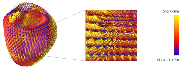
Figure 1.

A section of the reconstructed diffusion tensors in the LV lateral wall of the explanted donor heart. An individual tensor is represented by a glyph that is oriented in the principal directions (eigenvectors) of diffusion. The long axis of the glyph represents the fiber direction, and the glyph plane represents the fiber-sheet plane. The glyph axes are scaled by the normalized magnitude (eigenvalues) of diffusion along each principal axis. The glyph surfaces are colored based on the orientation of the fiber axis with respect to the circumferential axis.

2.3. Cardiovascular Model

The patient-specific cardiovascular model consists of four main components; an anatomic model of the ventricles, a passive constitutive model, an active contractile model, and a hemodynamic model (Figure (2)). The anatomic model of the ventricles in turn consists of the unloaded ventricular geometry, a volumetric scalar field that represents the scar region in the patient, and a fiber-sheet local material coordinate system that represent the myofiber and sheet architecture. The unloaded ventricular geometry is obtained by the unloading algorithm, which uses the ventricular geometry segmented and fitted from end-diastolic CT images and pressure measurements. The bi-ventricular geometry is a modeled as a 3D hexahedral cubic-Hermite finite-element mesh (128 elements, 209 nodes). The boundary conditions of the model were specified to prevent displacement and rotation of the base along the long axis. The scar region in the patient is modeled using a volumetric scalar field that directly corresponds to the perfusion density from MIBI-SPECT images; regions having a lower value than a predetermined perfusion density were considered scarred. The scarred region was modeled differently by changing the material parameters locally as explained in Section (2.4.3). Local fiber architecture was represented by a local myofiber-sheet material coordinate system calculated from the eigenvectors of the diffusion tensors interpolated in Log-Euclidian space. The diffusion-weighted images of the host donor-heart were registered to the corresponding ventricular model and the diffusion tensor was calculated at each node of the ventricle; it is then interpolated using Log-Euclidean metrics. This interpolated fiber architecture was then transformed to the patient-specific models using large deformation diffeomorphic maps from the host ventricular geometry to the target ventricular geometries.

Figure 2.

Different components of the patient-specific cardiovascular model and the various methods and data used in developing the model.

The second component of the patient-specific model consists of the constitutive law [20] for the resting myocardial material properties along with parameters that are adjusted to match the patient’s end-diastolic pressure-volume relations. The third component of the patient-specific model is the active-contractile law [29] that simulates muscle contraction. The parameters of this model were then adjusted to match the left and right-ventricular cavity pressures measured in the patient. The fourth component is the lumped-parameter closed-loop hemodynamic model [6] that generates the boundary condition for the ventricular finite-element model.

2.4. Patient-Specific Model Generation

This section presents the details of generating the patient-specific cardiac model based on the measured and empirical data available.

2.4.1. Bi-ventricular Geometry

Hexahedral cubic-Hermite finite element meshes of the ventricular geometries for each patient and the explanted host heart were constructed from the clinical and non-clinical image data. Endocardial and epicardial contours (left ventricle, right ventricle, septum, and epicardium) of the patient hearts at end-diastole were manually segmented from the CT images. The contours of the host heart were segmented from fractional anisotropy (FA) images of the DT-MRI scan to differentiate between myocardial and pericardial tissue such as fat; the two are otherwise indistinguishable in the null gradient images. Clear identification of myocardium is necessary to exclude the noise in the diffusion directions from non-myocardial regions.

An initial 2D cubic-Hermite template mesh (129 nodes, 108 elements) consisting of four nested surfaces representing the endocardial and epicardial surfaces was defined in prolate spheroidal coordinates. The geometry of the template mesh was pre-fitted to each patient by placing the nodes at common anatomical landmarks (left ventricular lateral wall, right ventricular lateral wall, base, apex, and the septum-right ventricular junctions) to preserve the structure of the mesh relative to each heart. Following Nielsen et al. [32], the pre-fitted meshes were fitted in the radial (λ) coordinate to the reconstructed data by a linear least squares minimization of the projection distance of the data to the interpolated mesh surfaces parameterized at the nodes.

The fitted surfaces were converted to hexahedral cubic-Hermite elements in rectangular Cartesian coordinates and re-fined transmurally to a final resolution of 209 nodes and 128 elements (5,016 geometric degrees of freedom) for both ventricles. The accuracy of the results was verified by ensuring that the RMS projection error was on the order of the spatial resolution of the image data (0.48 mm) and the LV cavity volume agreed to within 5% of the measured volume from the clinical data.

Infarct geometry and location was modeled by a volumetric scalar field representing perfusion density in the domain of the geometric model. The myocardial volume was segmented from the MIBI images, reconstructed in 3D space, and aligned with the previously constructed patient-specific ventricular mesh. The voxel intensities were mapped from their coordinates in the image stack to their locations within the ventricular mesh. The same linear least squares fit was performed to minimize the error between the measured perfusion density and the interpolated volumetric scalar field. The fitted perfusion map was thresholded to demarcate healthy and scarred regions of the myocardium. Heterogeneous passive and active material parameters characteristic of the mechanical properties of the two regions were assigned based on the map as explained in Section (2.4.3).

In addition, to compare the regional cardiac function between the model and measured data, ventricular geometry was also fitted to the echocardiographic images at end-diastole and end-systole [1]. The ventricular geometry was fitted to a low-resolution template mesh from two perpendicularly aligned echocardiographic images.

2.4.2. Ventricular Fiber Architecture

Diffusion tensor registration in the anatomical model

The diffusion tensor D is a 3 ×3 symmetric, positive-definite covariance matrix that represents the local voxel-averaged distribution of the diffusion of water molecules. Since the magnitude and principal directions of diffusion in tissue are physically constrained by the local micro-structure [7], one can infer the properties of this structure by decomposing D into its eigenvalues λ_i and eigenvectors v_i (i = 1, 2, 3), respectively.

Detailed histological studies [41, 25, 12] in isolated canine specimens have measured the anisotropic structure of the myocardium which consists of a mesh of myofibers embedded in laminar sheets separated by cleavage planes. Comparing histological measurements of the orientation of these fibers and sheets with results from DT-MRI measurements have confirmed that the fiber and sheet-normal directions coincide with the primary ([21], [19], [37]) and tertiary [17] eigenvectors. It is therefore feasible to represent the fiber-sheet directions in a model of the ventricle with a set of local orthogonal material coordinate axes calculated from the eigenvectors of interpolated diffusion tensors.

The problem of tensor interpolation is complicated by a number of factors. Tensor fields interpolated in normal Euclidean space may result in null or non-positive-definite interpolated tensors or artifacts such as swelling [14] that are not representative of real tissue structure [15]. Affine invariant Riemannian frameworks have been proposed which overcome these artifacts but are computationally expensive [34]. Tensor interpolation using a Log-Euclidian (LE) framework has the advantage of being much simpler to implement while preserving the positive definiteness, symmetry, and determinant of the diffusion tensor [5]. In the LE framework, the diffusion tensor D is transformed to L by the matrix logarithm: L = log(D); the symmetry and positive-definiteness of L is preserved. Computations in LE space such as interpolation of the components of L proceed in the same fashion as scalar quantities in Euclidian space.

The present fiber architecture model takes advantage of this implementation by directly interpolating the six independent components of L as separate 3D scalar fields fitted to the log-transformed components of the DT-MRI measurements in the domain of the cubic-Hermite mesh. The interpolated D is recovered by reassembling L from the interpolated fields and transforming it back to Euclidian space with the matrix exponential D = exp(L). D is finally decomposed into λ_i and v_i to obtain the fiber-sheet material axes.

The diffusion-tensor MRI measurements were registered into the anatomic mesh by first segmenting the myocardial area from the FA images described previously. In order to exactly align the segmented image volume with the anatomical model, overlapping voxels in the area and contour masks were used to compute the 4 ×4 affine transformation matrix T to rotate and translate the segmented volume. Since we are actually dealing with tensor images, the tensors themselves need to be reoriented to correct for the alignment to the anatomical model. A rotated tensor D′ is computed by applying the rotational component R of the affine transformation by D′ = R^T DR. The rotated tensor D′ was finally transformed to L′ in LE space, and their independent components were fitted by the same methods as the anatomical models.

Mapping the fiber architecture from the host to patient-specific models

A recent statistical analysis [26] of fiber architecture variation in a population of human hearts has revealed that fiber orientations are well preserved between individuals. This suggests that it is reasonable to model the fibers in a patient-specific anatomy with measurements from another human heart, after accounting for the variations in fiber orientation due to differences in ventricle size and shape. These geometric shape changes can be quantified between the anatomical models of the host and patient-specific hearts by large deformation diffeomorphic maps (LDDMs). Diffeomorphic transformations are smooth one-to-one mappings of one anatomical model domain to another that preserve geometric features [9]. Smoothness and bijectivity ensure that contours remain contours, surfaces remains surfaces, and volumes remain volumes through the transformation.

The present method employs high-order finite element 3D kinematic analysis to compute a parametrically represented large deformation diffeomorphic map between the host and target anatomical domains. A diffeomorphic map f transforms a material point Y in the host domain to point y (Y) in the target domain. The transformation f in a kinematic sense is equivalent to a field of deformation gradients F = ∂y_i/∂Y_j i, j = 1,2,3. Smoothness is satisfied if the Jacobian of F is nonsingular everywhere. The relative smoothness of f can be measured in terms of its harmonic energy [47] which is defined as the spatial averaging of the squared Frobenius norm of the Jacobian.

Application of the diffeomorphic transformation f on the fiber architecture requires a material coordinate reorientation strategy. The most suitable strategy is the so-called preservation of principal directions (PPD) [4]. Compared to the finite strain (FS) strategy, PPD reorients the fibers in a way that is more representative of the mechanical deformation in the reshaping of the host anatomy to the patient anatomy. In addition to the rotational component of F, PPD accounts for reorientation due to axial stretch and compression.

The fiber architecture transformation was implemented by calculating F between the host model and a patient model at the locations of the previously registered DT-MRI measurements. The interpolated material coordinate axes at these locations were reoriented according to the PPD strategy and recomposed into diffusion tensors D′ using the original λ_i; preservation of the eigenvalues is reasonable as it implies that tissue anisotropy is maintained during the deformation ([10]). The reoriented tensors were registered in the patient model and the local material coordinate system is computed in the same manner as the host heart (Figure (4)).

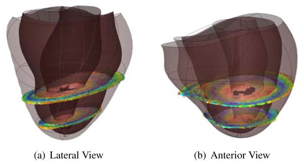
Figure 4.

Two views of the results of the large deformation diffeomorphic mapping and the tensor reorientation strategy from the host to a target patient (BiV4). The interpolated fiber architecture is shown in four transmural elements in the LV lateral wall. The fiber-sheets were reoriented using the PPD strategy by computing the deformation gradient F(Y) between corresponding material points in the host and the patient anatomical models.

2.4.3. Unloaded Bi-ventricular Geometry and Passive Material Properties

The in-vivo CT images are necessarily obtained in a loaded configuration of the heart; often end-diastole as defined by the peak of the R-wave. But, to compute stresses correctly, the unloaded reference state is required. This unloaded geometry, when loaded to the measured end-diastolic pressure, will deform to the measured end-diastolic geometry. This, in turn, depends on the material properties used for the myocardium. We have developed a method by which we can estimate the unloaded reference geometry given the end-diastolic geometry, pressure, and passive material properties. Previous studies have used some simplifying assumptions for the unloaded geometry; these include using the end-systolic [45] or mid-diastolic [39] geometry as the unloaded state. However, it was empirically observed that the unloaded volume is usually different than both these states [24]. Rajagopal et al. [35] developed a method to estimate the unloaded geometry of human breasts that has been applied to heart modeling by Nordsletten et al. [33]. They use a technique similar to 3-dimensional image registration to predict the unloaded state of the heart. However, their method does not guarantee the compatibility of the resulting unloaded geometry with the passive myocardial material properties. Recently, Alastrué et al. [2] have developed a method to find the unloaded geometry of vascular tissue based on the multiplicative decomposition of the deformation gradient tensor into an elastic and plastic component, typically applied in the modeling of growth [36].

In order to model the resting properties of the myocardium, we make use of the transversely-isotropic form of the constitutive model developed by Holzapfel and Ogden [20]. In this model, the anisotropy in the fiber and cross-fiber directions of the myocardium is modeled using a separate exponential term with different exponents. Equation (1) gives the equation for the strain energy.

$$\psi =\frac{a}{2b}{e}^{b(I_1-3)}+\frac{a_f}{2b_f}(e^{b_f{(I_{4f}-1)}^2}-1)$$ (1)

In Equation (1), I₁ corresponds to the first invariant of the right Cauchy-Green strain tensor, I_{4 f} corresponds to the components of the right Cauchy-Green strain tensor in the fiber direction. The parameters of the model were fitted to match the biaxial tests of Yin et al. [48] and the shear tests of Dokos et al. [13] of ex-vivo canine myocardial tissue. The default parameters of the transversely-isotropic model [20] resulted in too stiff stress-strain relations in the patient-specific models. Hence, the pressure scaling parameters (as) were scaled uniformly to fit the end-diastolic pressure volume relations in the patient-specific models. If the default parameters were still too non-linear for some patient-specific models, the exponential parameters were slightly altered (< 15%). The infarct region was also incorporated into the patient-specific ventricular models while generating the pressure-volume relations. The parameters in the infarct region were made stiffer by increasing the pressure scaling parameters (as) 10 times similar to Walker et al. [45].

Klotz et al. [24] reported an empirical relation for the unloaded left-ventricular cavity volume as a function of the end-diastolic pressure and cavity volume that was found to correlate well with measurements in human and animal hearts in health and under a wide variety of disease conditions (Equation (2)). We use this empirical relationship to scale the resting material parameters so that the left-ventricular cavity volume of the unloaded model matched the empirical value predicted by Klotz relation. Equation (2) gives the empirical relation for unloaded left-ventricular volume as a function of the measured end-diastolic pressure (in mm Hg) and the end-diastolic volume (in ml). In the current algorithm, if the computed unloaded volume is smaller than the empirical volume, the material stiffness is increased, and vice-versa.

$$V_0=(0.6-0.006P_m)V_m$$ (2)

Thus, given a set of material parameters, we find the unloaded geometry that when inflated to end-diastolic pressure, results in a loaded geometry that is the same as the mesh fitted to the end-diastolic state to within acceptable error limits. As shown in Figure (5), an initial guess for the unloaded state, X₀, is assumed to be the end-diastolic fitted mesh. This geometry was then inflated to the end-diastolic pressure to obtain the geometry Y₀. The inverse of the deformation gradient, F_YY0, between Y₀ and the fitted end-diastolic geometry, Y is then applied to the initial guess, X₀, to obtain a new estimate of the un-loaded geometry X₁ = [F_YY0]⁻¹ X₀. For each guess geometry, we also perform tensor reorientation to correctly transform the muscle fibers to the unloaded state. This process is iterated until the loaded geometry and the fitted end-diastolic geometries matched to within the measurement accuracy of the diastolic geometry.

Figure 5.

Algorithm to find the unloaded geometry. The initial geometry, X₀, is first inflated to the measured end-diastolic pressure. The deformation gradient between the inflated mesh (Y₀) and the fitted end-diastolic (Y) is then computed. This deformation gradient is then applied inversely to the initial estimate to get a new unloaded geometry estimate. This process is iterated until the projection error between the surfaces of the measured and loaded geometries is lower than the fitting error.

The key step of the algorithm is to apply the deformation gradient tensor inversely to get a new estimate of the unloaded geometry that is consistent with respect to the nodal positions of the initial geometry. However, it is not possible to perform this operation in a single step since the changes in the nodal positions are large. Therefore, the deformation gradient tensor is linearly decomposed and applied in steps to the estimated geometry to obtain the unloaded geometry.

$${[{\mathbf{F}}_{\mathbf{Y}{\mathbf{Y}}_{\mathbf{i}}}]}_k^{-1}=k{[{\mathbf{F}}_{\mathbf{Y}{\mathbf{Y}}_{\mathbf{i}}}]}^{-1}+(1-k)\mathbf{I}$$ (3)

Starting with our estimated geometry X_i, we apply [F_YYi]⁻¹ to obtain the new estimated geometry X_i+1. This operation is performed step-wise by decomposing [F_YYi]⁻¹ linearly with [I], starting with ${[{\mathbf{F}}_{\mathbf{Y}{\mathbf{Y}}_{\mathbf{i}}}]}_k^{-1}$, given by Equation (3) and k = 0. k is then incremented to a small value and the resulting deformation gradient is used to compute the stress in the geometry. The equilibrium solution for the position of the nodes that will reduce this stress to zero is then obtained. This new estimated geometry is also consistent with the resting material model. The value of k is then incremented and the process is repeated until the final unloaded geometry is obtained at k = 1.

Klotz et al. [24] also suggested a standardized volume normalization of the end-diastolic pressure-volume relation (ED-PVR) that eliminates most of the variation between individuals (including heart disease patients) and across species. They showed that the volume-normalized EDPVR can be approximated by power law expression (Equation (4)) for normal subjects and a wide range of pathologies including dilated car-diomyopathy. This relationship was used to validate the patient-specific unloaded geometry and the resting material properties.

$$\begin{array}{l}\mathit{EDP}=A_n{(\mathit{EDV})}^{B_n}\\ A_n=28.2mmHg\\ B_n=2.79\end{array}$$ (4)

2.4.4. Active Material Parameters and Hemodynamics

After the passive material parameters and unloaded geometry were obtained, the contractile parameters and the hemodynamic parameters were determined to match the measured peak left ventricular pressures and end-systolic volumes.

To adjust the active contraction parameters of the Lumens et al. [29] model, the finite element model was contracted iso-volumically by activating the fibers. The resulting pressure trace was compared with the measured catheter pressures in the patient and the parameters active stress scaling coefficient (SfAct), activation rise time (tR), and activation decay time (tD), were adjusted to match the peak systolic pressure, (dP/dt)_max, and (dP/dt)_min respectively.

The parameters of the circulation model are obtained independently using adaptation rules (CircAdapt [6]). The parameters can be separated into four categories (Figure (6)). The first category of parameters, such as mitral and aortic valve dimensions, are measured from echocardiographic data and input directly. Certain parameters such as atrial dimensions are predetermined from normal healthy human cardiac dimensions and are built-in as predetermined parameters in the model. These human cardiac measurements were supplemented with empirical data whenever direct measurements were not available. The third category of parameters, such as aortic length and pulmonary arterial length, are adjusted manually inside the CircAdapt algorithm to match the pressure measurements in the patient. Once these parameters are manually adjusted, the CircAdapt model uses its built-in simplified cardiac ventricular geometry model to adjust the remaining parameters to achieve the prescribed cardiac output and mean arterial pressure (Table (2)). The built-in cardiac ventricular geometry is then adjusted to match the ventricular cavity volumes from the finite-element model. The algorithm runs several cardiac cycles until a steady state that satisfies the prescribed conditions is reached. These new adapted parameters are then input to the closed-loop circulation model that is coupled to a patient-specific finite-element ventricular geometry model [22].

Figure 6.

Interaction between the circulation model and the finite-element ventricular model. Some of the circulation parameters that were measured in the patient are used directly. Then certain parameters are adjusted manually to match parameters such as end-diastolic and end-systolic pressures. The CircAdapt algorithm is used to estimate the remaining circulation parameters subject to constraints of cardiac output and mean aortic pressure. Finally, the adapted parameters are used in the circulation model coupled to finite element model. This process is iterated until the simulation results match the measured values.

3. Results

3.1. Patient-Specific Ventricular Anatomy

The DT-MRI measurements D(Y) of the donor heart were fitted to a corresponding anatomic model, and material axes were computed from the eigenvectors of the interpolated tensor D_i(Y) (Figure (7)).

Figure 7.

Lateral view of modeled fiber architecture fitted from DT-MRI measurements in a bi-ventricular model of the host heart. The diffusion tensors are represented as scaled glyphs depicting the orientation of the myofiber-sheet structure. The glyphs are colored according to their z-axis component. A close-up of lateral wall of the left ventricle reveals the well-established characteristic organization of the fibers through the thickness of the wall.

Tensor error metrics ([8], [3], [47]) were computed between D(Y) and D_i(Y) to evaluate the quality of the fiber fit. Let the eigenvalues and eigenvectors of a measured D be λ₁, λ₂, λ₃ (λ₁ > λ₂ > λ₃) and v₁, v₂ and v₃, respectively. The eigen-values and eigenvectors of an interpolated D_i are similarly ${\lambda }_1^{\prime },{\lambda }_2^{\prime },{\lambda }_3^{\prime }$ and $v_1^{\prime },v_2^{\prime }$ and $v_3^{\prime }$. Metrics on the diffusion tensor were computed as the norm of the absolute error in Euclidean and log Euclidian space. Metrics on tensor shape, which are functions of the eigenvalues, include absolute errors in fractional anisotropy, logarithmic fractional anisotropy, apparent diffusion coefficient, volume, linear anisotropic diffusion coefficient, planar anisotropic diffusion coefficient, spherical anisotropic diffusion coefficient, relative anisotropy, volume ratio, dispersion, and the eigenvalues themselves. Since the local fiber transformation relies on the eigenvectors of D_i(Y), the most relevant error metric is the overlap error between $v_i^{\prime }$ and v_i (Equation (5)).

$$1-\frac{{\sum }_{i=1}^3{\lambda }_i{\lambda }_i^{\prime }{(v_i·v_i^{\prime })}^2}{{\sum }_{i=1}^3{\lambda }_i{\lambda }_i^{\prime }}.$$ (5)

A histogram of the overlap error is shown in Figure (8). Histograms of the remaining error metrics are displayed in the Appendix Figure (A.16). Linear interpolation of the log-Euclidean components of D_i in the cubic-Hermite domain of the donor model registered 112,419 of 152,651 DT measurements (74%) with an overlap error less than 0.3; the highest agreement occurred in the LV, septum, and apex (Figure (9)) where the quality of measurements was high. Linear basis functions were sufficient to capture the characteristic variation of fiber and sheet orientation where the quality of measurements is high. Areas of poor overlap occurred in the right ventricle where measurements were less reliable. The base of the anterior right ventricle in particular had a very thin wall that had been folded over during the DT-MRI scan.

Figure 8.

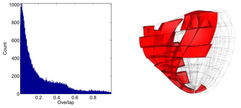
Distribution of the overlap error tensor metric between the measured and modeled material axes at corresponding locations in the model. Regions with poor overlap are marked in the bi-ventricular host mesh on the right.

Figure 9.

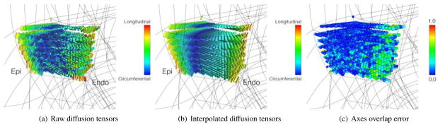
(a) Raw diffusion tensor data in four transmural elements located in the LV lateral wall. (b) Interpolated diffusion tensors from the fit of the log-Euclidean components. (c) Degree of overlap between (a) and (b). Points of high overlap are colored blue; points of lower overlap are colored green. Note the fit smoothing achieved by linear interpolation of the DT components.

MIBI scans of patients BiV2 and BiV4 were registered to their anatomical models (Figure (10)), and the scar locations were confirmed by clinical experts. The scar location for BiV5 was not available from MIBI data and was instead identified on the anatomical model by a clinical expert.

Figure 10.

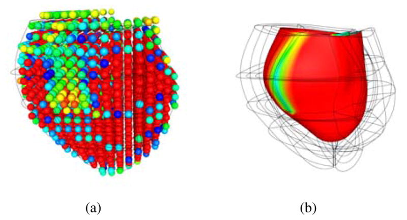
(a) The voxel intensities of the MIBI scan were reconstructed in 3D space and aligned to the anatomical model of the ventricles. (b) A scalar field was fitted to the voxel intensities to define the region of the scar on the posterior left ventricular lateral wall running from base to mid-ventricle in BiV4.

3.2. Unloaded Geometry and Passive Parameters

The unloading algorithm was used to estimate the patient-specific unloaded ventricular geometry. In order to test the convergence of the method to a valid geometry, the error between the inflated geometry obtained from the unloaded geometry and the fitted end-diastolic geometry was computed. A dense set of points on the surfaces of inflated geometry (LV endocardium, RV endocardium, septum, and the epicardium) was first computed and then projected to the closest point on the corresponding surfaces of the fitted geometry. The projection error is then computed by finding the average projection length. Figure (11) shows the average projection error as a function of the number of iterations of the algorithm. It can be seen that the error is lower than the fitting error within 6 iterations. The inset figure shows the regional distribution of the projection error. It can be seen that the projection error is maximum in the septal wall region. This might be because of a poor fit in that region of the end-diastolic geometry that leads to the septal wall being fitted at unrealistic angles with respect to the LV and RV.

Figure 11.

The error in the unloading algorithm is measured using the average projection distance between the points on the surface of the fitted end-diastolic mesh and the loaded mesh. This error reaches a value lower than the fitting error within a few iterations. The inset figure shows the regional distribution of the error.

The patient-specific parameters of the constitutive model were also estimated together with the unloaded geometry. The estimated parameters are given in Table (3). It can be seen that the parameters for all the five patients are very similar, but softer than the canine properties reported in [20]. This might be either due to the softening of tissue associated with matrix metallo-proteinase activity in heart failure [40], or due to the hardening of the originally tested canine tissue samples due to the effects of rigor, edema and cutting injury.

Figure (12) shows the end-diastolic pressure-volume relationships of the five patient-specific models. It can be seen that the anisotropic characteristics of the patient-specific model is similar to the one predicted empirically by Klotz et al. [24].

Figure 12.

End-diastolic pressure-volume relationships for five different patient specific models. The dotted lines represent the shape of the curve using Klotz’s empirical relationship. The chosen model and material parameters were able to reproduce the fitted curves.

3.3. Closed-Loop Ventricular Simulations

The patient-specific models were used to simulate several cardiac cycles and the global measures such as ejection fraction and mitral regurgitation volume were compared with echocardiographic and Doppler measurements (Table (4)). Figure (13) compares the LV and RV cavity pressures of the model with pressure measurements from cardiac catheterization. It can be seen that the parameters such as peak-pressure, (dP/dt)_max, and (dP/dt)_min are captured by the patient-specific model. Figure (13(b)) shows the corresponding LV and RV pressure-volume loops for the cardiac cycle for patient BiV2. The difference in the total stroke volume of the two cavities can be used as a measure of the mitral valve regurgitation volume, since it was assumed that there was no tricuspid valve regurgitation.

Figure 13.

Comparison of the measured and simulated LV and RV cavity pressures and pressure-volume loops for one of the patients. Individual plots are included in the Appendix.

The ventricular geometries fitted to echocardiographic images at end-diastole and end-systole were used to compare regional geometry changes such as the radial displacement. Since these echocardiographic images were not used for the modeling, they serve as an independent validation of the model. Figure (14) shows the radial displacement at the different regions of the left-ventricle between end-diastole and end-systole. The standard left-ventricular segmentation nomenclature [11] was used to compare the results. It can be seen that the average values are consistent between the model and Echocardiographic measurements and the average error is less than 0.4 cm for all patients. In addition, the error is relatively high near the base of the ventricles. This might be due to the difficulty in correctly identifying the base plane while segmenting the 2D echocardiographic data for some patients.

Figure 14.

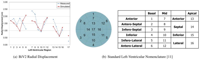
Radial displacement between end-diastole and end-systole from the measured and simulated geometries at different locations of the left-ventricle for one of the patients. The radial displacement in the simulated model closely matches the values obtained from models fitted to echocardiographic images.

Figure (15) directly compares the results of one of the patient specific models (BiV2) by overlaying the images of the simulated heart (brown) over the echocardiographic images. It can be seen that the model accurately matches the measured images at end-diastolic and end-systolic states.

Figure 15.

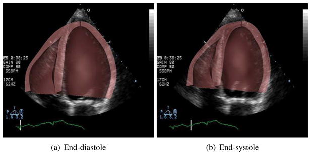
Comparison of ventricular geometry of the simulated heart (brown), overlaid on the clinical echocardiographic images of the same heart at end-diastole and end-systole.

4. Discussion

In this paper, we present new semi-automated methods that can be integrated to develop bi-ventricular models of patient-specific biomechanics in the failing heart. The modeling pipeline described here integrates many clinical and non-clinical measurements –including CT imaging, echocardiography, cardiac catheterization, MIBI-SPECT, and DT-MRI– to develop a detailed patient-specific model. A model of human ventricular and sheet architecture was reconstructed from DT-MR images of a human organ-donor heart and mapped to the patient-specific ventricular model. Resting myocardial material properties and the unloaded reference ventricular geometry for stress analysis were determined simultaneously to match empirical relations that have been reported previously to be well conserved between normal and diseased individuals [24]. Systolic contractile material parameters were determined to match left ventricular pressure measurements and end-systolic volumes. Circulation parameters were estimated using adaptation rules (CircAdapt) constrained by measured cardiac output, mean arterial pressure, and aortic and mitral valve dimensions. The closed-loop circulation model was then coupled to the finite-element ventricular model to simulate complete cardiac cycles. We tested these methods in five patients with heart failure that was also complicated by myocardial infarction, mitral valve regurgitation, and electrical dyssynchrony. In the present study, we made use of available data on mitral valve regurgitation and myocardial infarct size and location, but we did not attempt to model the electrical dyssynchrony.

Other workers have also developed methods for developing patient-specific models of the failing heart [38, 31]. The utility of such models is that they can be used to predict global parameters as well as regional function of the heart, some of which cannot be directly measured in the patient. However, none of those previous studies made use of human ventricular myofiber orientations, nor did they solve a boundary value problem to determine the unloaded ventricular geometry. While these earlier studies did couple the finite element model of the ventricle to a lumped parameter model of the circulation, they did not use a closed-loop circulatory model. Some previous researchers Nordsletten et al. [33] have made use of the empirical observations by Klotz et al. [24] that we used, but here we formalized this information to estimate the myocardial material parameters and solve for the unloaded reference geometry simultaneously.

Here we used human DT-MRI measurements in an ex-vivo heart to reconstruct a model of the fiber-sheet anatomy that was mapped to the patient models to define local material coordinate axes. It has been shown that the fiber architecture is usually conserved over a wide range of conditions between individuals [46]. However, we did not take into account the diseased state of the patients’ hearts. It has been shown that fiber directions are more dispersed in abnormal hearts [27]. Recently, in-vivo DT-MRI measurements [42] were used to reconstruct myocardial fiber architecture. Those workers used a diffeomorphic demons algorithm to map DT-MRI measurements to a prolate-spheroidal model of the left ventricle and an anisotropic kernel estimator to interpolate regions of sparse measurements from the mid ventricle to the apex. However, reliable measurements were restricted by the image quality to the region between the base and mid-ventricle where cardiac motion was least. Nevertheless, there is the promise to reconstruct patient-specific models of in-vivo fiber architecture, with improved in-vivo imaging. The techniques used here should be useful for registering and interpolating in-vivo DT-MR images.

We were unable to quantitatively validate the reconstructed fiber anatomy with histological measurements, though others have reported good agreement between fiber and sheet-normal directions with the principal directions (primary and tertiary, respectively) of water diffusion measured using DT-MRI [37, 17, 18]. We also cannot validate the registration of the ex-vivo data to the patient-specific cardiac model, however other workers [44] have validated the use of diffeomorphic maps and similar tensor reorientation strategies to transfer the myofiber architecture between anatomical models.

The unloading algorithm makes use of a linear decomposition of the deformation gradient tensor that was applied in steps. However, this means that the unloading curve that the material follows is different from the loading curve. An equally valid method is to compute the residual forces that can keep the geometry in equilibrium after applying the deformation gradient and then gradually reduce these forces to zero. This method was also implemented in one of the patient-specific ventricular geometries and it was found that both the methods gave very similar unloaded geometries. This suggests that the method is independent of the decomposition of the deformation gradient tensor.

In reality a heart - under normal conditions - will always contain residual stresses. However, the numerical method employed (finite elasticity) requires a reference state that is unstressed and unloaded, even in the case when residual stresses would have been included. In the current study, we did not include residual stresses, because these are unknown and can be introduced in multiple ways ([23]). However, it would be an interesting study where residual stresses are included in some way in determining an unloaded (but not unstressed) geometry for the purpose of patient-specific cardiac mechanics.

Since multiple sources provide the same data (such as CT, Echocardiography etc. for anatomic data), there might be some inconsistency in the measured data. We made use of data obtained at a higher resolution in such cases. For example, we rely on CT images to reconstruct the geometry over 2D echocardiographic images. The cases where data is not available due to poor quality of measurements (such as valve dimensions) we rely on empirical measurements. This is a limitation of the current method; however, one that cannot be avoided since perfect high-resolution clinical data is not always available. Finally, conflicted data sources were resolved with the help of a clinical specialist. A possible future study would be to identify the subset of the data that is sufficient to model the function in patient-specific hearts without loss of detail.

While most of the measured clinical data were used to formulate the patient-specific models, independent measurements of regional wall displacements from the clinical echocardiographic recordings were available for comparison with the model results. Regional variations in wall motion computed in the models followed a similar pattern to the measurements, though there appeared to be a consistent error in displacements near the base. It is possible that the echocardiographic reconstruction and the CT-derived derived patient model were not properly registered. Another source of inconsistency between the model results and measurements is the presence of dyssynchrony in the five patients. Dyssynchrony might also account for some of the regional variations between simulations and measurements. However, one of the patients in our previous study [1], is the same as the patient BiV2 in the current study. We had previously modeled the dyssynchrony, but the biomechanics did not include high-resolution ventricular geometry from CT images, human fiber architecture, or mitral valve regurgitation. However, we found that on including the dyssynchrony to our current model, global parameters such as the peak left-ventricular cavity pressure decreased by at most 10%. This indicates that new material parameters estimated by taking into account the dyssynchrony will not differ by a large value. In addition, the methodology that we have presented in this study to build patient-specific models will still be the same with suitable additions to the cardiovascular model to account for the dyssynchrony.

Instead of performing a sensitivity analysis on parameter values, we have estimated the error at each step and adjusted the parameters to reduce them. The geometry is reconstructed from high-resolution CT images. The parameters of the passive material properties (2 independent parameters) were adjusted while simultaneously obtaining the unloaded geometry. The error in this step is reduced by matching the empirical end-diastolic pressure-volume relations. Finally, the active material properties (4 independent parameters) and hemodynamic properties were adjusted to match ventricular pressures and end-systolic volumes. Again, the parameters were adjusted to reduce the error between the model and measured pressures with the error in the peak pressure being less than 5% for all patients. In addition, for the hemodynamic parameters, we make use of adaptation rules (CircAdapt) that reduce the total number of parameters. The input parameters for the CircAdapt algorithm have been subject to a sensitivity analysis before ([6]). Finally, considering that we have pressure measurements at each point in the cardiac cycle coupled with empirical end-diastolic pressure-volume relations, we can be sure of getting a fit for all the model parameters.

Some of the methods such as segmentation are still performed manually that can lead to some systematic errors. Automated methods such as deformable registration could be used to automate this process. In addition, some of the methods such as determination of the hemodynamic parameters are performed independently that might lead to some variation between the estimated and actual parameters. This can be better solved with the help of an optimization algorithm that can find the parameters that match the model output with measurements.

In conclusion, we have demonstrated the viability of creating detailed patient-specific models to perform biomechanics simulations. The models are capable of replicating patient-specific global cardiac functions. The main goal of this paper is to define the requirements of a patient-specific model, and to develop the model. However, once such a model that simulates function in the normal heart is developed, it can be modified and the effects of different interventions could be studied with the goal of predicting treatments for heart disease with a computational model.

Figure 3.

Two views of the fitted anatomic model of the host heart with 2 reconstructed slices from the DT-MRI scan aligned to it before fitting the tensor component fields. The slices were precisely aligned with the anatomic model of the host heart and the tensors were rotated to account for the alignment.

Table 1.

Summary of each patient’s clinical assessment.

Data	BiV2	BiV3	BiV4	BiV5	BiV6
Forward Ejection Fraction (%)	25	26	24	22	33
Mitral Regurgitant Volume (ml)	16	-	36	14	-
Heart Rate (bpm)	70	70	70	60	70
Infarct Location	Inferior, Septal	-	Anterior, Lateral, Basal	Inferior, Septal, Apical	-

Table 2.

Geometric and functional data used as input to the CircAdapt algorithm before adaptation. This data was obtained from Doppler and echocardiographic measurements.

Data	BiV2	BiV3	BiV4	BiV5	BiV6
Cardiac cycle length (ms)	860	860	860	1000	860
Cardiac output (ml/sec)	51.0	64.0	84.0	52.0	55.0
Mean aortic pressure (kPa)	13.2	13.0	17.0	11.0	10.0
Mitral valve diameter (cm)	1.61	2.16	2.30	4.21	2.50
Aortic valve diameter (cm)	1.84	2.04	2.38	2.21	2.50
Aortic diameter (cm)	3.37	-	-	-	-

Table 3.

Passive parameters of the Ogden-Holzapfel models optimized for the patient-specific models. The ratios of the parameters were not changed to maintain the anisotropy. The a parameters are very similar between the patients.

Data	BiV2	BiV3	BiV4	BiV5	BiV6
a (kPa)	0.684	0.912	0.730	0.912	0.684
b (−)	9.726	8.267	9.726	8.267	9.726
af (kPa)	0.510	0.674	0.539	0.674	0.510
bf (−)	15.779	13.412	15.779	13.412	15.779

Table 4.

Comparison of global parameters for the patient-specific models with echocardiographic measurements.

Parameter	BiV2		BiV3		BiV4		BiV5		BiV6
	Meas.	Sim.	Meas.	Sim.	Meas.	Sim.	Meas.	Sim.	Meas.	Sim.
Forward Ejection Fraction (%)	25	22	23	26	24	21	22	25	33	31
Mitral Regurgitation Volume (ml)	16	10	-	-	36	30	14	10	-	-

Appendix A. Diffusion Tensor Error Metrics

Tensor error metrics were computed between the DT-MRI measurements D(Y) of the donor heart and the eigenvectors of the interpolated tensor D_i(Y) to evaluate the quality of the fiber fit. The eigenvalues and eigenvectors of measured D are λ₁, λ₂, λ₃ (λ₁ > λ₂ > λ₃) and v₁, v₂ and v₃, respectively. The eigen-values and eigenvectors of the interpolated D_i are similarly ${\lambda }_1^{\prime },{\lambda }_2^{\prime },{\lambda }_3^{\prime }$ and $v_1^{\prime },v_2^{\prime }$ and $v_3^{\prime }$. Metrics on the diffusion tensor were computed as the norm of the absolute error in Euclidean and log Euclidian space. Metrics computed include absolute errors in fractional anisotropy (FA), logarithmic fractional anisotropy (LFA), apparent diffusion coefficient (ADC), volume (Vol), linear anisotropic diffusion (C_L), planar anisotropic diffusion (C_P), spherical anisotropic diffusion (C_S), relative anisotropy (RA), volume ratio (VR), dispersion, and the eigenvalues themselves [47]. These metrics are reported in Figure (A.16).

Figure A.16.

Diffusion tensor error metrics to assess the quality of the fitted diffusion tensor field compared to original measurements.

Appendix B. Simulation Results

Here we present all the simulation results for the five patients. Figure (B.17) gives the simulated and measured, left and right ventricular pressures for all the patients. Figure (B.18) shows their corresponding pressure-volume loops. Finally, Figure (B.19) shows the radial displacement between end-diastole and end-systole at different left-ventricular regions using the standard nomenclature [11].

Figure B.17.

Comparison of the measured and simulated LV and RV cavity pressures in the five patients. The RV measurement in patient BiV5 was not reliable due to fluctuations in the measurements.

Figure B.18.

Pressure-volume loops for the five patient-specific models.

Figure B.19.

Radial displacement between end-diastole and end-systole from the measured and simulated geometries at different locations of the left-ventricle.

References

- 1.Aguado-Sierra J, Krishnamurthy A, Villongco C, Chuang J, Howard E, Gonzales M, Omens J, Krummen D, Narayan S, Kerckhoffs R, et al. Patient-specific modeling of dyssynchronous heart failure: A case study. Progress in Biophysics and Molecular Biology. 2011 doi: 10.1016/j.pbiomolbio.2011.06.014. [DOI] [PMC free article] [PubMed] [Google Scholar]
- 2.Alastrue V, Garía A, Peña E, Rodríguez J, Martínez M, Doblaré M. Numerical framework for patient-specific computational modelling of vascular tissue. International Journal for Numerical Methods in Biomedical Engineering. 2010;26 (1):35–51. [Google Scholar]
- 3.Alexander A, Hasan K, Kindlmann G, Parker D, Tsuruda J. A geometric analysis of diffusion tensor measurements of the human brain. Magnetic Resonance in Medicine. 2000;44 (2):283–291. doi: 10.1002/1522-2594(200008)44:2<283::aid-mrm16>3.0.co;2-v. [DOI] [PubMed] [Google Scholar]
- 4.Alexander D, Pierpaoli C, Basser P, Gee J. Spatial transformations of diffusion tensor magnetic resonance images. Medical Imaging, IEEE Transactions on. 2001;20 (11):1131–1139. doi: 10.1109/42.963816. [DOI] [PubMed] [Google Scholar]
- 5.Arsigny V, Fillard P, Pennec X, Ayache N. Fast and simple calculus on tensors in the log-euclidean framework. Medical Image Computing and Computer-Assisted Intervention–MICCAI. 2005;2005:115–122. doi: 10.1007/11566465_15. [DOI] [PubMed] [Google Scholar]
- 6.Arts T, Delhaas T, Bovendeerd P, Verbeek X, Prinzen F. Adaptation to mechanical load determines shape and properties of heart and circulation: the CircAdapt model. American Journal of Physiology-Heart and Circulatory Physiology. 2005;288 (4):H1943. doi: 10.1152/ajpheart.00444.2004. [DOI] [PubMed] [Google Scholar]
- 7.Basser P. Inferring microstructural features and the physiological state of tissues from diffusion-weighted images. NMR in Biomedicine. 1995;8 (7):333–344. doi: 10.1002/nbm.1940080707. [DOI] [PubMed] [Google Scholar]
- 8.Basser P, Pajevic S. Statistical artifacts in diffusion tensor mri (dt-mri) caused by background noise. Magnetic Resonance in Medicine. 2000;44 (1):41–50. doi: 10.1002/1522-2594(200007)44:1<41::aid-mrm8>3.0.co;2-o. [DOI] [PubMed] [Google Scholar]
- 9.Cao Y, Miller M, Winslow R, Younes L. Large deformation diffeomorphic metric mapping of vector fields. Medical Imaging, IEEE Transactions on. 2005;24 (9):1216–1230. doi: 10.1109/tmi.2005.853923. [DOI] [PubMed] [Google Scholar]
- 10.Cao Y, Miller MI, Mori S, Winslow RL, Younes L. Diffeomorphic matching of diffusion tensor images. Computer Vision and Pattern Recognition Workshop. 2006:67. doi: 10.1109/CVPRW.2006.65. [DOI] [PMC free article] [PubMed] [Google Scholar]
- 11.Cerqueira M, Weissman N, Dilsizian V, Jacobs A, Kaul S, Laskey W, Pennell D, Rumberger J, Ryan T, Verani M. Standardized myocardial segmentation and nomenclature for tomographic imaging of the heart. Circulation. 2002;105 (4):539–542. doi: 10.1161/hc0402.102975. [DOI] [PubMed] [Google Scholar]
- 12.Costa K, Takayama Y, McCulloch A, Covell J. Laminar fiber architecture and three-dimensional systolic mechanics in canine ventricular myocardium. American Journal of Physiology-Heart and Circulatory Physiology. 1999;276 (2):H595. doi: 10.1152/ajpheart.1999.276.2.H595. [DOI] [PubMed] [Google Scholar]
- 13.Dokos S, Smaill B, Young A, LeGrice I. Shear properties of passive ventricular myocardium. American Journal of Physiology-Heart and Circulatory Physiology. 2002;283 (6):H2650. doi: 10.1152/ajpheart.00111.2002. [DOI] [PubMed] [Google Scholar]
- 14.Fillard P, Arsigny V, Pennec X, Ayache N. Joint estimation and smoothing of clinical DT-MRI with a Log-Euclidean metric. 2006. [DOI] [PubMed] [Google Scholar]
- 15.Fillard P, Pennec X, Arsigny V, Ayache N. Clinical DT-MRI estimation, smoothing, and fiber tracking with Log-Euclidean metrics. IEEE Trans Med Imaging. 2007;26 (11):1472–82. doi: 10.1109/TMI.2007.899173. [DOI] [PubMed] [Google Scholar]
- 16.Frank L, Jung Y, Inati S, Tyszka J, Wong E. High efficiency, low distortion 3D diffusion tensor imaging with variable density spiral fast spin echoes 3D DW VDS RARE. Neuroimage. 2010;49 (2):1510–1523. doi: 10.1016/j.neuroimage.2009.09.010. [DOI] [PMC free article] [PubMed] [Google Scholar]
- 17.Helm P, Beg M, Miller M, Winslow R. Measuring and mapping cardiac fiber and laminar architecture using diffusion tensor MR imaging. Annals - New York Academy of Sciences. 2005;1047:296. doi: 10.1196/annals.1341.026. [DOI] [PubMed] [Google Scholar]
- 18.Helm P, Tseng H, Younes L, McVeigh E, Winslow R. Ex vivo 3d diffusion tensor imaging and quantification of cardiac laminar structure. Magnetic resonance in medicine. 2005;54 (4):850–859. doi: 10.1002/mrm.20622. [DOI] [PMC free article] [PubMed] [Google Scholar]
- 19.Holmes A, Scollan D, Winslow R. Direct histological validation of diffusion tensor MRI in formaldehyde-fixed myocardium. Magnetic resonance in medicine. 2000;44 (1):157–161. doi: 10.1002/1522-2594(200007)44:1<157::aid-mrm22>3.0.co;2-f. [DOI] [PubMed] [Google Scholar]
- 20.Holzapfel G, Ogden R. Constitutive modelling of passive myocardium: a structurally based framework for material characterization. Philosophical Transactions A. 2009;367 (1902):3445. doi: 10.1098/rsta.2009.0091. [DOI] [PubMed] [Google Scholar]
- 21.Hsu E, Muzikant A, Matulevicius S, Penland R, Henriquez C. Magnetic resonance myocardial fiber-orientation mapping with direct histological correlation. American Journal of Physiology-Heart and Circulatory Physiology. 1998;274 (5):H1627. doi: 10.1152/ajpheart.1998.274.5.H1627. [DOI] [PubMed] [Google Scholar]
- 22.Kerckhoffs R, Neal M, Gu Q, Bassingthwaighte J, Omens J, Mc-Culloch A. Coupling of a 3D finite element model of cardiac ventricular mechanics to lumped systems models of the systemic and pulmonic circulation. Annals of Biomedical Engineering. 2007;35 (1):1–18. doi: 10.1007/s10439-006-9212-7. [DOI] [PMC free article] [PubMed] [Google Scholar]
- 23.Kerckhoffs RC. Computational modeling of cardiac growth in the post-natal rat with a strain-based growth law. Journal of Biomechanics. 2012;45 (5):865– 871. doi: 10.1016/j.jbiomech.2011.11.028. [DOI] [PMC free article] [PubMed] [Google Scholar]
- 24.Klotz S, Hay I, Dickstein ML, Yi GH, Wang J, Maurer MS, Kass DA, Burkhoff D. Single-beat estimation of end-diastolic pressure-volume relationship: a novel method with potential for noninvasive application. American Journal of Physiology - Heart and Circulatory Physiology. 2006;291 (1):H403–H412. doi: 10.1152/ajpheart.01240.2005. [DOI] [PubMed] [Google Scholar]
- 25.LeGrice I, Smaill B, Chai L, Edgar S, Gavin J, Hunter P. Laminar structure of the heart: ventricular myocyte arrangement and connective tissue architecture in the dog. American Journal of Physiology-Heart and Circulatory Physiology. 1995;269 (2):H571. doi: 10.1152/ajpheart.1995.269.2.H571. [DOI] [PubMed] [Google Scholar]
- 26.Lombaert H, Peyrat J, Croisille P, Rapacchi S, Fanton L, Clarysse P, Delingette H, Ayache N. Statistical analysis of the human cardiac fiber architecture from DT-MRI. Functional Imaging and Modeling of the Heart. 2011:171–179. [Google Scholar]
- 27.Lombaert H, Peyrat J-M, Fanton L, Cheriet F, Delingette H, Ayache N, Clarysse P, Magnin I, Croisille P. Statistical atlas of human cardiac fibers: comparison with abnormal hearts. Proceedings of the Second international conference on Statistical Atlases and Computational Models of the Heart: imaging and modelling challenges; Springer-Verlag. 2012. pp. 207–213. [Google Scholar]
- 28.Lumens J, Blanchard D, Arts T, Mahmud E, Delhaas T. Left ventricular underfilling and not septal bulging dominates abnormal left ventricular filling hemodynamics in chronic thromboembolic pulmonary hypertension. American Journal of Physiology-Heart and Circulatory Physiology. 2010;299 (4):H1083. doi: 10.1152/ajpheart.00607.2010. [DOI] [PubMed] [Google Scholar]
- 29.Lumens J, Delhaas T, Kirn B, Arts T. Three-wall segment (TriSeg) model describing mechanics and hemodynamics of ventricular interaction. Annals of Biomedical Engineering. 2009;37 (11):2234–2255. doi: 10.1007/s10439-009-9774-2. [DOI] [PMC free article] [PubMed] [Google Scholar]
- 30.Neal M, Kerckhoffs R. Current progress in patient-specific modeling. Briefings in bioinformatics. 2010;11 (1):111. doi: 10.1093/bib/bbp049. [DOI] [PMC free article] [PubMed] [Google Scholar]
- 31.Niederer SA, Plank G, Chinchapatnam P, Ginks M, Lamata P, Rhode KS, Rinaldi CA, Razavi R, Smith NP. Length-dependent tension in the failing heart and the efficacy of cardiac resynchronization therapy. Cardiovascular Research. 2011;89 (2):336–43. doi: 10.1093/cvr/cvq318. [DOI] [PubMed] [Google Scholar]
- 32.Nielsen P, LeGrice I, Smaill B, Hunter P. Mathematical model of geometry and fibrous structure of the heart. American Journal of Physiology- Heart and Circulatory Physiology. 1991;260 (4):H1365. doi: 10.1152/ajpheart.1991.260.4.H1365. [DOI] [PubMed] [Google Scholar]
- 33.Nordsletten DA, Niederer SA, Nash MP, Hunter PJ, Smith NP. Coupling multi-physics models to cardiac mechanics. Progress in Biophysics and Molecular Biology. 2011;104 (1–3):77–88. doi: 10.1016/j.pbiomolbio.2009.11.001. [DOI] [PubMed] [Google Scholar]
- 34.Pennec X, Fillard P, Ayache N. A riemannian framework for tensor computing. Int’l Journal of Computer Vision. 2006;66 (1):41–66. [Google Scholar]
- 35.Rajagopal V, Chung J, Nielsen P, Nash M. Finite element modelling of breast biomechanics: directly calculating the reference state. Engineering in Medicine and Biology Society, 2006. EMBS’06. 28th Annual International Conference of the IEEE; IEEE. 2006. pp. 420–423. [DOI] [PubMed] [Google Scholar]
- 36.Rodriguez E, Hoger A, McCulloch A. Stress-dependent finite growth in soft elastic tissues. Journal of biomechanics. 1994;27 (4):455–467. doi: 10.1016/0021-9290(94)90021-3. [DOI] [PubMed] [Google Scholar]
- 37.Scollan D, Holmes A, Zhang J, Winslow R. Reconstruction of cardiac ventricular geometry and fiber orientation using magnetic resonance imaging. Annals of Biomedical Engineering. 2000;28 (8):934–944. doi: 10.1114/1.1312188. [DOI] [PMC free article] [PubMed] [Google Scholar]
- 38.Sermesant M, Peyrat J, Chinchapatnam P, Billet F, Mansi T, Rhode K, Delingette H, Razavi R, Ayache N. Toward patient-specific myocardial models of the heart. Heart Failure Clinics. 2008;4 (3):289–301. doi: 10.1016/j.hfc.2008.02.014. [DOI] [PubMed] [Google Scholar]
- 39.Sermesant M, Razavi R. Personalized computational models of the heart for cardiac resynchronization therapy. Patient-Specific Modeling of the Cardiovascular System. 2010:167–182. [Google Scholar]
- 40.Spinale F, Coker M, Bond B, Zellner J. Myocardial matrix degradation and metalloproteinase activation in the failing heart: a potential therapeutic target. Cardiovascular research. 2000;46 (2):225. doi: 10.1016/s0008-6363(99)00431-9. [DOI] [PubMed] [Google Scholar]
- 41.Streeter D, Jr, Spotnitz H, Patel D, Ross J, Jr, Sonnenblick E. Fiber orientation in the canine left ventricle during diastole and systole. Circulation research. 1969;24 (3):339. doi: 10.1161/01.res.24.3.339. [DOI] [PubMed] [Google Scholar]
- 42.Toussaint N, Sermesant M, Stoeck CT, Kozerke S, Batchelor PG. In vivo human 3D cardiac fibre architecture: reconstruction using curvilinear interpolation of diffusion tensor images. Med Image Comput Comput Assist Interv. 2010;13 (Pt 1):418–25. doi: 10.1007/978-3-642-15705-9_51. [DOI] [PubMed] [Google Scholar]
- 43.Trayanova N. Whole heart modeling. Circulation Research. 2011;108 (1):113–128. doi: 10.1161/CIRCRESAHA.110.223610. [DOI] [PMC free article] [PubMed] [Google Scholar]
- 44.Vadakkumpadan F, Gurev V, Constantino J, Arevalo H, Trayanova N. Modeling of whole-heart electrophysiology and mechanics: Toward patient-specific simulations. Patient-Specific Modeling of the Cardiovascular System. 2010:145–165. [Google Scholar]
- 45.Walker J, Ratcliffe M, Zhang P, Wallace A, Fata B, Hsu E, Saloner D, Guccione J. MRI-based finite-element analysis of left ventricular aneurysm. American Journal of Physiology-Heart and Circulatory Physiology. 2005;289 (2):H692. doi: 10.1152/ajpheart.01226.2004. [DOI] [PubMed] [Google Scholar]
- 46.Weis S, Emery J, Becker K, McBride D, Jr, Omens J, McCulloch A. Myocardial mechanics and collagen structure in the osteogenesis imperfecta murine (oim) Circulation Research. 2000;87 (8):663–669. doi: 10.1161/01.res.87.8.663. [DOI] [PubMed] [Google Scholar]
- 47.Yeo B, Vercauteren T, Fillard P, Peyrat J, Pennec X, Golland P, Ayache N, Clatz O. DT-REFinD: Diffusion tensor registration with exact finite-strain differential. Medical Imaging, IEEE Transactions on. 2009;28 (12):1914–1928. doi: 10.1109/TMI.2009.2025654. [DOI] [PMC free article] [PubMed] [Google Scholar]
- 48.Yin F, Strumpf R, Chew P, Zeger S. Quantification of the mechanical properties of noncontracting canine myocardium under simultaneous biaxial loading. Journal of biomechanics. 1987;20 (6):577–589. doi: 10.1016/0021-9290(87)90279-x. [DOI] [PubMed] [Google Scholar]