A linear optimal transportation framework for quantifying and visualizing variations in sets of images

Abstract

Transportation-based metrics for comparing images have long been applied to analyze images, especially where one can interpret the pixel intensities (or derived quantities) as a distribution of ‘mass’ that can be transported without strict geometric constraints. Here we describe a new transportation-based framework for analyzing sets of images. More specifically, we describe a new transportation-related distance between pairs of images, which we denote as linear optimal transportation (LOT). The LOT can be used directly on pixel intensities, and is based on a linearized version of the Kantorovich-Wasserstein metric (an optimal transportation distance, as is the earth mover’s distance). The new framework is especially well suited for computing all pairwise distances for a large database of images efficiently, and thus it can be used for pattern recognition in sets of images. In addition, the new LOT framework also allows for an isometric linear embedding, greatly facilitating the ability to visualize discriminant information in different classes of images. We demonstrate the application of the framework to several tasks such as discriminating nuclear chromatin patterns in cancer cells, decoding differences in facial expressions, galaxy morphologies, as well as sub cellular protein distributions.

1 Introduction

1.1 Background and motivation

Automated image analysis methods are often used for extracting important information from image databases. Common applications include mining information in sets of microscopy images [22], understanding mass distribution in celestial objects from telescopic images [34], as well as analysis of facial expressions [36], for example. We note that the prevalent technique for quantifying information in such large datasets has been to reduce the entire information (described by pixel intensity values) contained in each image in the database to a numerical feature vector (e.g. size, form factor, etc.). Presently, this approach (coupled with clustering, classification, and other machine learning techniques) remains the prevalent method through which researchers extract quantitative information about image databases and cluster important image subgroups [6,44,19].

In addition to feature-based methods, several techniques for analyzing image databases based on explicit modeling approaches have recently emerged. Examples include contour-based models [29], medial axis models [8], as well as model-based deconvolution methods [15]. Moreover, when analyzing images within a particular type (e.g. brain images) researchers have often used a more geometric approach. Here the entire morphological exemplar as depicted in an image is viewed as a point in a suitably constructed metric space (see for example [4]), often facilitating visualization. These approaches have been used to characterize the statistical variation of a particular object in a given population (or set of populations) [4,24]. The main idea in these is to understand the variation of similar objects through analysis of the deformation fields required to warp one object (as depicted in its image) onto another.

Alternatively, transportation-based metrics have also been used to analyze image data in problems when pixel intensities (or derived quantities) can be interpreted as ‘mass’ free to move without strict geometric constraints [32,18,11,16,43]. They are interesting alternatives to other methods since when applied directly to pixel intensities, they have the potential to quantify both texture and, to some extent, shape information combined (see for example [18,43]). In particular, there has been continuing effort to develop fast and reliable methods for computing transportation related distances [26,20, 35,28,2,3,5,12,17]. While the computational complexity of these methods ranges from quadratic to linear with respect to image size (for smooth enough images), the computations are still expensive (time wise), in particular for rough images (with large gradients), and there are issues with convergence (e.g. due to local minima in PDE-based variational implementations).

1.2 Overview of our approach and contributions

Our contribution is to develop a linear framework closely related to the optimal transportation metric (OT) [43] for analyzing sets of images. This framework, which we call the linear optimal transportation (LOT), not only provides a fast way for computing a metric (and geodesics) between all pairs in a dataset, permitting one to use pixel intensities directly, but it also provides an isometric embedding for a set of images. Therefore our method takes as input a potentially large set of images and outputs an isometric embedding of the dataset (endowed with the LOT metric) onto the standard Euclidean space. Our approach achieves this task by utilizing the following series of steps:

• Step 1: compute a template image that will serve as a reference point for analyzing the given image dataset.

• Step 2: for each image in the input dataset, as well as the estimated template, compute a particle approximation that will enable a linear programming-based computation of the OT distance between it and the template computed in STEP 1.

• Step 3: normalize each particle approximation with respect to translation, rotation, and coordinate inversions.

• Step 4: compute a quadratic-based OT distance between the particle approximation of each image and the template.

• Step 5: from the output of STEP 4, compute the LOT distances and embedding.

As compared to previous works that make use of transportation-related metrics in image analysis, we highlight the following innovations of our approach. The first is that, given a database of M images, the number of transportation related optimizations required for computing the distance between all pairs of images is M when utilizing our approach (versus M(M − 1)/2 when utilizing other approaches). This provides a substantial increase in speed especially when performing pattern recognition tasks (e.g. classification) in large databases. Secondly, as mentioned above, our LOT framework also provides an isometric linear embedding that has a couple of convenient properties. One being that the embedding of an image newly added to the database can be computed exactly and with one transportation optimization only. Another being that any point in the embedded space can be visualized as an image. This includes measured points (existing images in the database) but also any other point in this space. Below we show how this embedding greatly facilitates the use of standard geometric data analysis techniques such as principal component analysis (PCA) and linear discriminant analysis (LDA) for visualizing interesting variations in a set of images.

1.3 Paper organization

In section 2 we begin by reviewing the mathematical underpinnings of the traditional optimal transportation framework and then describe its linearized version and some of its properties. Equation (1) gives the definition of the traditional OT metric, and formulas (2) and (3) the linearized version of the metric. Then in section 3 we describe our computational approach in the discrete setting. This includes an algorithm for ‘estimating’ the content of a relatively sparse image with particles (full details of this algorithm are provided in appendix A). The definition of the OT distance in the discrete setting is provided in equation (5), while our approximation of its linearized version in the discrete setting is given in formula (9). Equations (10) and (11) provide the isometric linear embedding for a given particle approximation according to a reference point. Section 4 describes how one can utilize the linear embedding provided in the LOT framework to extract useful information from sets of images using principal component analysis and linear discriminant analysis. The applications of LOT towards decoding subcellular protein patterns and organelle morphology, galaxy morphology as well as facial expression differences are presented in section 5.

2 Optimal transportation framework

Transportation-based metrics are especially suited for quantifying differences between structures (depicted in quantitative images) that can be interpreted as a distribution of mass with few strict geometric constraints. More precisely, we utilize the optimal transportation (Kantorovich-Wasserstein) framework to quantify how much mass, in relative terms, is distributed in different regions of the images. We begin by describing the mathematics of the traditional OT framework, and in particular the geometry behind it, which is crucial to our subsequent introduction of the linearized OT distance.

2.1 Optimal transportation metric

Let Ω represent the domain (the unit square [0, 1]², for example) over which images are defined. To describe images we use the mathematical notion of a measure. While this is somewhat abstract, it enables us to treat simultaneously the situation when we consider the image to be a continuous function and when we deal with actual computations and consider the image as a discrete array of pixels. It is important for us to do so, because many notions related to optimal transportation are simpler in the continuous setting, and in particular we can give an intuitive explanation for the LOT distance we introduce. On the other hand the discrete approximation necessitates considering a more general setting because the mass (proportional to intensity) from one pixel during transport often needs to be redistributed over several pixels.

We note that, in the current version of the technique, we normalize all images in a given dataset so that the intensity of all pixels in each image sums to one. Thus we may interpret images as probability measures. The assumption is adequate for the purpose of analyzing shape and texture in the datasets analyzed in this paper. We note that OT-related distances can be used when masses are not the same [32,27].

Recall that probability measures are nonnegative and that the measure of the whole set Ω is 1: μ(Ω) = ν(Ω) = 1. Let c: Ω × Ω → [0, ∞) be the cost function. That is c(x, y) is the ‘cost’ of transporting unit mass located at x to the location y. The optimal transportation distance measures the least possible total cost of transporting all of the mass from μ to ν. To make this precise, consider Π(μ, ν), the set of all couplings between μ and ν. That is consider the set of all probability measures on Ω × Ω with the first marginal μ and the second marginal ν. More precisely, if π ∈ Π(μ, ν) then for any measurable set A ⊂ Ω we have π(A × Ω) = μ(A) and π(O×A) = ν(A). Each coupling describes a transportation plan, that is π(A₀ × A₁) is telling one how much ‘mass’ originally in the set A₀ is being transported into the set A₁.

We consider optimal transportation with quadratic cost c(x, y) = |x−y|². The optimal transportation (OT) distance, also known as the Kantorovich-Wasserstein distance, is then defined by

$$d_W(\mu ,\nu )={\left(\underset{\pi \in \mathrm{\Pi }(\mu ,\nu )}{inf}{\int }_{\mathrm{\Omega }\times \mathrm{\Omega }}{\mid x-y\mid }^{2}d\pi \right)}^{\frac{1}{2}}.$$ (1)

It is well known that the above infimum is attained and that the distance defined is indeed a metric (satisfying the positivity, the symmetry, and the triangle inequality requirements), see [39]. We denote the set of minimizers π above by Π_OT(μ, ν).

2.2 Geometry of optimal transportation in continuous setting

The construction of the LOT metric which we introduce below, can be best motivated in the continuous setting. Consider measures μ and ν which have densities α and β, that is

$$d\mu =\alpha (x)dx\text{and}d\nu =\beta (x)dx.$$

Then the following mathematical facts, available in [39], hold. The OT plan between μ and ν is unique and furthermore the mass from each point x, is sent to a single location, given as the value of the function ϕ(x) called the optimal transportation map (see Figure 1). The relation between ϕ and the optimal transportation plan Π introduced above is that Π(A₀ × A₁) = μ({x ∈ A₀ : ϕ(x) ∈ A₁}). That is Π is concentrated on the graph of ϕ. We note that ϕ is a measure preserving map from μ to ν, that is that for any A, ∫_ϕ⁻¹(A)α(x)dx = ∫_A β(y)dy. The Kantorovich-Wasserstein distance is then d_W(μ, ν) = ∫_ω|ϕ(x) − x|²α(x)dx.

Fig. 1.

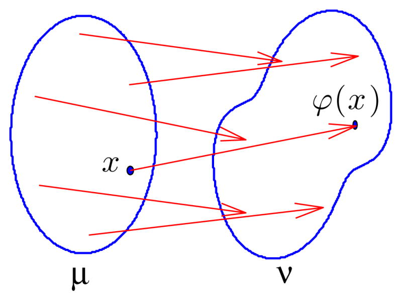
Optimal transport map ϕ between measures μ and ν whose supports are outlined.

In addition to being a metric space the set of measures is formally a Riemannian manifold [10], that is at any point there is a tangent space endowed with an inner product. In particular the tangent space at the measure σ with density γ (i.e. dσ = γ(x)dx) is the set of the following vector fields T_σ = {v : Ω → ℝ^d such that ∫_Ω|v(x)|²γ(x)dx < ∞} and the inner product is the weighted L²:

$${\langle v_1,v_2\rangle }_{\sigma }={\int }_{\mathrm{\Omega }}{v}_1(x)·v_2(x)\gamma (x)dx.$$

The OT distance is just the length of the shortest curve (geodesic) connecting two measures [5].

A very useful fact is the geodesics have a form that is simple to understand. Namely if μ_t, 0 ≤ t ≤ 1 is the geodesic connecting μ to ν. Then μ_t is the measure obtained when mass from μ is transported by the transportation map x → (1−t)x+tϕ(x). Then ${\mu }_t(A)={\int }_{{\varphi }_t^{-1}(A)}\alpha (x)dx$.

2.3 Linear optimal transportation metric

Computing a pairwise OT distance matrix is expensive for large datasets. In particular let T_OT be the time it takes to compute the OT distance and T₂ the time it takes to compute the Euclidean distance between two moderately complex images. Using the method described below, T_OT is typically on the order of tens of seconds, while T₂ is on the order of miliseconds. For a dataset with M images, computing the pairwise distances takes time on the order of M(M − 1)T_OT/2. Here we introduce a version of the OT distance that is much faster to compute. In particular computing the distance matrix takes approximately MT_OT + M (M − 1)T₂/2. For a large set of images, in which the number of pixels in each image is fixed, as the number of images in the set tends to infinity, the dominant term is M²T₂.

The distance we compute is motivated by the geometric nature of the OT distance. Heuristically, instead of computing the geodesic distance on the manifold we compute a ‘projection’ of the manifold to the tangent plane at a fixed point and then compute the distances on the tangent plane. This is the main reason we use the term linear when naming the distance. To consider the projection one needs to fix a reference image σ (where the tangent plane is set). Computing the projection for each image requires computing the OT plan between the reference image σ and the given image. Once computed, the projection provides a natural linear embedding of the dataset, which we describe in section 3.5.

We first describe the LOT distance in the continuous setting. Let σ be a probability measure with density γ. We introduce the identification (‘projection’), P, of the manifold with the tangent space at σ. Given a measure μ, consider the optimal transportation map ψ between σ and μ. Then

$$P(\mu )=v\text{where}v(x)=\psi (x)-x.$$

Note that v ∈ T_σ and that P is a mapping from the manifold to the tangent space. See Figure 2 for a visualization. Also P(σ) = 0 and $d_W{(\sigma ,\mu )}^2={\int }_{\mathrm{\Omega }}{\mid \psi (x)-x\mid }^2\gamma (x)dx={\int }_{\mathrm{\Omega }}{\mid v(x)\mid }^2\gamma (x)dx={\langle v,v\rangle }_{\sigma }={\left|\right|P(\mu )-P(\sigma )\left|\right|}_{\sigma }^2$, were ${\left|\right|v\left|\right|}_{\sigma }^2$ is defined to be 〈v, v〉_σ. So the mapping preserves distances to σ. Let us mention that in cartography such projection is known as the equidistant azimuthal projection. In differential geometry this would be the inverse of the exponential map. We define the LOT as:

$$d_{\mathit{LOT}}(\mu ,\nu )={\left|\right|P(\mu )-P(\nu )\left|\right|}_{\sigma }.$$ (2)

Fig. 2.

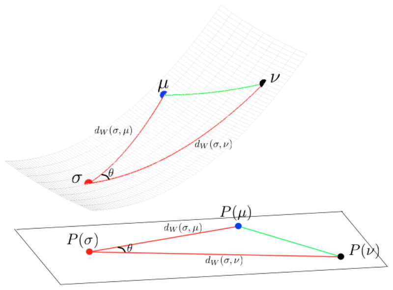
The identification of the manifold with the tangent plane. Distances to σ as well as angles at σ are preserved.

When σ is not absolutely continuous with respect to the Labesgue measure the situation is more complicated. The purely discrete setting (when the measures are made of particles) is the one relevant for computations and we discuss it in detail in section 3.3. In the general setting, the proper extension of the LOT distance above is the shortest generalized geodesic (as defined in [1]) connecting μ and ν. More precisely, given a reference measure σ, and measures μ and ν, with transportation plans π_μ ∈ Π_OT(σ, μ) and π_ν ∈ Π_OT(σ, ν), let Π(σ, μ, ν) be the set of all measures on the product Ω × Ω × Ω such that the projection to first two co-ordinates is π_μ and the projection to the first and the third is π_ν. The linearized version of the OT distance between μ and ν is given by:

$$d_{\mathit{LOT},\sigma }{(\mu ,\nu )}^2=\underset{\pi \in \mathrm{\Pi }(\sigma ,\mu ,\nu )}{inf}{\int }_{\mathrm{\Omega }\times \mathrm{\Omega }\times \mathrm{\Omega }}{\mid x-y\mid }^{2}d\pi .$$ (3)

2.4 Translation and Rotation normalization

It is important to note that the OT metric defined in equation (1) is not invariant under translations or rotations. It can be rendered translation invariant by simply aligning all measures in a dataset μ₁, ···, μ_N by setting their center of mass to a common coordinate. This is based on the fact that if μ is a measure on Ω with center of mass

$$x_{\mu }=\frac{1}{\mu (\mathrm{\Omega })}{\int }_{\mathrm{\Omega }}xd\mu$$

and ν a measure of the same mass, then among all translates of the measure ν, ν_x(A) = ν(A − x), the one that minimizes the distance to μ is the one with the center of mass x_μ.

From now on, we will always assume that the measures are centered at the origin (the implementation of this normalization step is given below). The Euclidean-transformation invariant Kantorovich-Wasserstein distance is then defined in the following way. Given a measure μ and an orthogonal matrix T, define μ_T by μ_T(A) = μ(T⁻¹ A). Then the invariant distance is defined by d(μ, ν) = min_T∈O(n) d_W(μ_T, ν). In two dimensions we have developed an algorithm for finding the minimum above. However we know of no reasonable algorithm for computing the rotation invariant linearized OT distance (d_LOT). Below we present an algorithm that greatly reduces the effect of rotation, but does not eliminate it completely.

3 Computing LOT distances from image data

To compute the LOT distance for a set of images we need to first compute the OT distance from a template image to each of the images. There exist several approaches for computing OT distances. Perhaps the most direct idea is to discretize the problem defined in (1). This results in a linear programming problem (see (5) below). While this approach is very robust and leads to the global minimizer, it is computationally expensive (the fastest strongly polynomial algorithm for this case is the Hungrian algorithm with time complexity of O(n³) with n the number of pixels in an image). Other approaches are based on continuum ideas, where PDEs and variational techniques are often used [2,3,5,12,17]. Some of them achieve close to linear scaling with the number of pixels. On the other hand, their performance can deteriorate as one considers images that lack regularity (are not smooth, have large gradients). A particular difficulty with some of the approaches that are not based on linear programing is that they may not converge to the global solution if they arrive at a local minimum first.

Our approach is based on combining linear programming with a particle approximation of the images. It is a refinement of the algorithm we used in [43]. That is, each image is first carefully approximated by a particle measure (a convex combination of delta masses) that has much fewer particles than there are pixels in the image. This significantly reduces the complexity of the problem. Furthermore it takes advantage of the fact that many images we consider are relatively sparse. Then one needs fewer particles for accurate approximation of the image which accelerates the computation. In addition, as the number of particles approaches the number of pixels in the image, the approximation error tends to zero. We now present the details of the algorithm. In particular, we give a description of the particle approximation, and detailed algorithms for translation and rotation normalization, and the computation of the LOT distance. The full details pertaining to the particle approximation algorithm, which is more involved, are presented in Appendix A.

3.1 Particle approximation

The first step in our computational approach is to represent each image as a weighted combination of ‘particles’ each with mass (intensity) m_i and location x_i:

$$\mu =\sum _{i=1}^{N_{\mu }}{m}_i{\delta }_{x_i}.$$ (4)

with N_μ being the number of masses used to represent the measure (image) μ. Since the images are digital, each image could be represented exactly using the model above by selecting m_i to be the pixel intensity values and δ_xi the pixel coordinate grid. Given that images can contain a potentially large number of pixels, and that the cost of a linear programing solution for computing the OT is generally $O(N_{\mu }^3)$, we do not represent each image exactly and instead choose to approximate them.

The goal of the algorithm is to use at most, approximately, N particles to approximate each image, while maintaining a similar approximation error (by approximation error we mean the OT distance between the image and the particle approximation) for all images of a given dataset. For a dataset of M images, our algorithm requires the user to specify a number N for the approximate number of particles that could be used to approximate any image, and consists of these four steps:

• Step 1: use a weighted K-means algorithm [21] to approximate each image, with the number of clusters set to the chosen N. As we describe in the appendix, the weighted K-means is an optimal local step for reducing the OT error between a given particle approximation and an image.

• Step 2: improve the approximation of each image by investigating regions where each image is not approximated well, and add particles to those regions to improve the approximation locally. Details are provided in Appendix A.

• Step 3: compute the OT distance between each digital image and the approximation of each image. For images not well approximated by the current algorithm (details provided in Appendix A), add particles to improve the approximation.

• Step 4: For images where the approximation error is significantly smaller than the average error (for the entire dataset) remove (merge) particles until the error between the digital image and its approximation is more similar to the other images. (This reduces the time to compute the distances, while it does not increase the typical error.)

The algorithm above was chosen based on mathematical observations pertaining to the OT metric. These observations, including a careful description of each of the steps above, are provided in Appendix A. We have experimented with several variations of the steps above, and through this experience we have converged on the algorithm presented. A few of the details of the algorithm could be improved further, though we view further improvements to be beyond the scope of this paper. We emphasize that this particle approximation algorithm works particularly well for relatively sparse images, and less so for non-sparse (e.g. flat) images. Bellow we demonstrate, however, that the algorithm can nonetheless be used to extract meaningful quantitative information for datasets of images which are not sparse.

Translation and rotation normalization

In two dimensions, it suffices to consider translation, rotation, and mirror symmetry. To achieve that we simply align the center of mass of each particle approximation to a fixed coordinate, and rotate each particle approximation to a standard reference frame according to a principal axis (Hotteling) transform. Each particle approximation is then flipped left to right, and up and down, simply by reversing their coordinates, until the skewness (the third standardized moment) of the coordinates of each sample have the same sign.

3.2 OT distance in particle setting

We start by explaining how the general framework of section 2 applies to particle measures (such as particle approximations obtained above). A particle probability measure, μ, which approximates the image is given as $\mu ={\sum }_{i=1}^N{m}_i{\delta }_{x_i}$ where x_i ∈ Ω, m_i ∈ (0, 1], ${\sum }_{i=1}^N{m}_i=1$.

We note that for A ⊂ Ω, μ(A) = Σ_{i:xi ∈ A}m_i. An integral with respect to measure μ is ∫_A f(x)dμ(x) = Σ_{i:xi ∈ A} f(x_i)m_i.

Now we turn to our main goal of the section: obtaining the OT distance. For $\mu ={\sum }_{i=1}^{N_{\mu }}{m}_i{\delta }_{x_i}$ and $\nu ={\sum }_{j=1}^{N_{\nu }}{p}_j{\delta }_{y_j}$ the set of couplings Π(μ, ν) is given by a set of N_μ × N_ν matrices, as follows:

$$\mathrm{\Pi }(\mu ,\nu )=\{\sum _{i=1}^{N_{\mu }}\sum _{j=1}^{N_{\nu }}{f}_{i,j}{\delta }_{x_i,y_j}:f_{i,j}\ge 0\text{for}i=1,\dots ,N_{\mu },j=1,\dots ,N_{\nu }\sum _{j=1}^{N_{\nu }}{f}_{i,j}=m_i\text{for}i=1,\dots ,N_{\mu }\sum _{i=1}^{N_{\mu }}{f}_{i,j}=p_j\text{for}j=1,\dots ,N_{\nu }\}.$$

Since it is clear from the context we will make no distinction between measures in Π(μ, ν) and matrices f = [f_i,j] that satisfy the conditions above.

The optimal transportation distance between μ and ν defined in (1) is the solution to the following linear programing problem:

$$d_W^2(\mu ,\nu )=\underset{f\in \mathrm{\Pi }(\mu ,\nu )}{min}\sum _{i=1}^{N_{\mu }}\sum _{j=1}^{N_{\nu }}{\mid x_i-y_j\mid }^2{f}_{i,j}.$$ (5)

See Figure 3 for a visualization. For convenience, we utilize Matlab’s implementation of a variation of Mehrotras dual interior point method [23] to solve the linear program. We note however that better suited alternatives, which take advantage of the special structure of the linear programming problem, exist and could be used [26,32] to increase the computational efficiency of the method even further. The solution of the linear program above is relatively expensive [43], with typical computation times being around 30 seconds (with 500 particles per image) on an Apple laptop with a 2.2GHz intel dual core processor and 2GB of RAM.

Fig. 3.

When measures are discrete as in (4), then finding the transportation plan which minimizes the transportation cost, (5), necessitates splitting the particles. The arrows are drawn only for positive f_i,j.

For datasets containing tens of thousands of images this is practical only if we need to compute a single OT distance per image (the one to the reference image), and is prohibitive if we need the pairwise distance between all images. This is the reason we introduce the linear optimal transportation framework to compute a related distance between μ and ν.

3.3 LOT distance in particle setting

Computing the linear optimal transportation (LOT) distance requires setting a reference template σ, which we also choose to be a particle measure $\sigma ={\sum }_{k=1}^{N_{\sigma }}{q}_k{\delta }_{z_k}$ (how the reference template is computed is described in section 3.4). The distance between μ and ν given by (3) in a discrete setting becomes:

$$d_{\mathit{LOT},\sigma }{(\mu ,\nu )}^2=\underset{f\in {\mathrm{\Pi }}_{OT}(\sigma ,\mu ),g\in {\mathrm{\Pi }}_{OT}(\sigma ,\nu )}{min}\underset{h}{min}\{\sum _{i=1}^{N_{\mu }}\sum _{j=1}^{N_{\nu }}\sum _{k=1}^{N_{\sigma }}{h}_{k,i,j}{\mid x_i-y_j\mid }^2:\text{where}{h}_{k,i,j}\ge 0,\sum _{i=1}^{N_{\mu }}{h}_{k,i,j}=g_{k,j}\text{and}\sum _{j=1}^{N_{\nu }}{h}_{k,i,j}=f_{k,i}\}$$ (6)

We remark that the sets of optimal transportation plans, Π_OT(σ, μ) and Π_OT(σ, ν), typically have only one element, so there is only one possibility for f, and g. See Figure 4 for a visualization. Usually there is more than one possibility for h, in the case of particle measures.

Fig. 4.

Given f and g in (6), for each k fixed, h_k,i,j gives the optimal transportation plan between the ‘f-image’ and the ‘g-image’ of the particle at z_k. Arrows are drawn only for positive coefficients, and only for the particle at z_k.

We now introduce the ‘distance’ which is an approximation of the one above (hence we denote it as d_aLOT) and which is used in most computations in this paper. Namely, given OT plans f and g, as indicated in Figure 5, we replace the f-image of the particle at z_k, namely the measure Σ_i f_k,iδ_xi, by one particle at the center of mass, namely the measure q_kδ_x̂k. We recall from Section 2.2 that if σ, μ and ν were measures which had a density function (and hence no particles) then there exists an optimal transportation map and the image of any z is just a single x. On the discrete level we have an approximation of that situation and typically the f-image of the particle at z_k is spread over a few nearby particles. Thus the error made by replacing the f image by a single particle at the images center of mass is typically small.

Fig. 5.

For the LOT distance we replace the full f-image and the g-image of the particle at z_k by their centers of mass x̂_k and ŷ_k, (7). When there are many particles the images of particle at z_k tend to be concentrated on a few nearby particles. Thus the error introduced by replacing them by their center of mass is small.

To precisely define the new distance, let f be an optimal transportation plan between $\sigma ={\sum }_{k=1}^{N_{\sigma }}{q}_k{\delta }_{z_k}$ and $\mu ={\sum }_{i=1}^{N_{\mu }}{m}_i{\delta }_{x_i}$ obtained in (5), and g is an optimal transportation plan between $\sigma ={\sum }_{k=1}^{N_{\sigma }}{q}_k{\delta }_{z_k}$ and $\nu ={\sum }_{j=1}^{N_{\nu }}{p}_j{\delta }_{x_j}$. Then

$${\overline{x}}_k=\frac{1}{q_k}\sum _{i=1}^{N_{\mu }}{f}_{k,i}{x}_i\text{and}{\overline{y}}_k=\frac{1}{q_k}\sum _{j=1}^{N_{\nu }}{g}_{k,j}{y}_j$$ (7)

are the centroids of the forward image of the particle q_kδ_zk by the transportation plans f and g respectively (see Figure 5). We define

$$d_{\mathit{aLOT},\sigma }{(\mu ,\nu )}^2=\underset{\begin{array}{l}f\in {\mathrm{\Pi }}_{OT}(\sigma ,\mu )\\ g\in {\mathrm{\Pi }}_{OT}(\sigma ,\nu )\end{array}}{min}\sum _{k=1}^{N_{\sigma }}{q}_k{\mid {\overline{x}}_k-{\overline{y}}_k\mid }^2$$ (8)

We clarify that computing (8) in practice does not require a minimization over f and g, since f and g are unique with probability one. The reason for that is that in the discrete case the condition for optimality of transportation plans can be formulated in terms of cyclic monotonicity (see [40]). The nonuniuqueness of the OT plan can only happen if the inequalities in some cyclic monotonicity conditions become equalities, which means that the coordinates of particles satisfy an algebraic equation. And this can only happen with probability zero. For example, if both measures have exactly two particles of the same mass then the condition for nonuniqueness is that |x₁ − y₁|² + |x₂ − y₂|² = |x₂ − y₁|² + |x₁ − y₂|².

Thus we compute

$$d_{\mathit{aLOT},\sigma }{(\mu ,\nu )}^2=\sum _{k=1}^{N_{\sigma }}{q}_k{\mid {\overline{x}}_k-{\overline{y}}_k\mid }^2.$$ (9)

One should notice that the d_aLOT,σ distance between two particle measures may be zero. This is related to the ‘resolution’ achieved by the base measure σ. In particular if σ has more particles then it is less likely that d_aLOT,σ(μ, ν) = 0 for μ ≠ ν. It is worth observing that d_aLOT,σ(μ, ν)² computed in (9) is always less than or equal to d_LOT,σ(μ, ν)² introduced in equation (6).

Furthermore if we consider measures with continuous density σ, μ, and ν and approximate them by particle measures σ_n, μ_n, and ν_n, then as the number of particles goes to infinity d_LOT,σn(μ_n, ν_n) → d_LOT,σ (μ, ν) where the latter object is defined in (2). This follows from the stability of optimal transport [40].

Let us also remark that, while we use the linear programming problem as described in (5) to compute the optimal transportation plan, other methods can be used as well. In particular the LOT distance is applicable even when a different approach to computing the OT plan is used.

3.4 Template selection

Selecting the template (reference) σ above is important since, in our experience, a template that is distant from all images (particle approximations) is likely to increase the difference between d_W and d_aLOT. In the results presented below, we use a reference template computed from the ‘average’ image. To compute such average image, we first align all images to remove translation, rotation, and horizontal and vertical flips, as described in Section 3.3. All images are then averaged, and the particle approximation algorithm described above is used to obtain a particle representation of the average image. We denote this template as σ and note that it will contain N_σ particles. Once the particle approximation for the template is computed, it is also normalized to a standard position and orientation as described above.

3.5 Isometric linear embedding

When applying our approach to a given a set of images (measures) I₁, ···, I_M, we first compute the particle approximation for each image with the algorithm described in section 3.1. We then compute a template σ as described in section 3.4 and compute the OT distance (5) between a template σ (also chosen to be a particle measure) and the particle approximation of each image. Once these are computed, the LOT distance between any two particle sets is given by (9).

The lower bound of the linear optimal transportation distance d_aLOT,σ defined in equation (9) provides a method to map a sample measure ν_n (estimated from image I_n) into a linear space. Let ${\nu }_n={\sum }_{j=1}^{N_{{\nu }_n}}{m}_j{\delta }_{y_j}$ and recall that the reference measure is $\sigma ={\sum }_{k=1}^{N_{\sigma }}{q}_k{\delta }_{z_k}$. The linear embedding is obtained by applying the discrete transportation map between the reference measure σ and ν_n to the coordinates y_j via

$${\mathbf{x}}_n={\left(\sqrt{q_1}{a}_n^1\cdots \sqrt{q_{N_{\sigma }}}{a}_n^{N_{\sigma }}\right)}^T$$ (10)

where a^k is the centroid of the forward image of the particle q_kδ_kk by the optimal transportation plan, g_k,j, between images σ and ν_n:

$$a_n^k=\sum _{j=1}^{N_{{\nu }_n}}{g}_{k,j}{y}_j/q_k$$ (11)

This results in an N_σ-tuple of points in ℝ² which we call the linear embedding x_n of ν_n. That is, x_n ∈ ℝ^N_σ×2. We note that the embedding is interpretable in the sense that any point in this space can be visualized by simply plotting the vector coordinates (each in ℝ²) in the image space Ω.

4 Statistical analysis

When a linear embedding for the data can be assumed, standard geometric data processing techniques such as principal component analysis (PCA) can be used to extract and visualize major trends of variation in morphology [8,33,38]. Briefly, given a set of data points x_n, for n = 1, ···, M, we can compute the covariance matrix $S=\frac{1}{M}{\sum }_n({\mathbf{x}}_n-\overline{\mathbf{x}}){({\mathbf{x}}_n-\overline{\mathbf{x}})}^T$, with $\overline{\mathbf{x}}=\frac{1}{M}{\sum }_{n=1}^M{\mathbf{x}}_n$ representing center of the entire data set. PCA is a method for computing the major trends (directions over which the projection of the data has largest variance) of a dataset via the solution of the following optimization problem:

$${\mathbf{w}}_{\mathit{PCA}}^{\ast }=arg\underset{\left|\right|\mathbf{w}\left|\right|=1}{max}{\mathbf{w}}^{T}S\mathbf{w}$$ (12)

The problem above can be solved via eigenvalue and eigenvector decomposition, with each eigenvector corresponding to a major mode of variation in the dataset (it’s corresponding eigenvalue is the variance of the data projected over that direction).

In addition to visualizing the main modes of variation for a given dataset, important applications involve visualizing the modes of variation that best discriminate between two or more separate populations (e.g. as in control vs. effect studies). To that end, we apply the methodology we developed in [41], based on the well known Fisher linear discriminant analysis (FLDA) technique [14]. As explained in [41], simply applying the FLDA technique in morphometry visualization problems can lead to erroneous interpretations, since the directions computed by the FLDA technique are not constrained to pass through the data. To alleviate this effect we modified the method as follows. Briefly, given a set of data points x_n, for n = 1, ···, N, with each index n belonging to class c, we modified the original FLDA by adding a least squares-type representation penalty in the function to be optimized. The representation constrained optimization can then be reduced to

$${\mathbf{w}}_{\mathit{LDA}}^{\ast }=arg\underset{\mathbf{w}}{max}\frac{{\mathbf{w}}^T{S}_T\mathbf{w}}{{\mathbf{w}}^T(S_W+\alpha \mathbf{I})\mathbf{w}}$$ (13)

where S_T = Σn (x_n − x̂)(x_n − x̂)^T represents the ‘total scatter matrix’, S_W = Σ_c Σ_n∈c (x_n − x̂_c) (x_n − x̂_c)T represents the ‘within class scatter matrix’, x̂_c is the center of class c. The solution for the problem above is given by the well-known generalized eigenvalue decomposition S_T w = λ(S_W + αI) w [7]. In short, the penalized LDA method above seeks to find the direction w that has both a low reconstruction error, but that best discriminates between two populations. We use the method described in [41] to select the penalty weight α.

5 Computational results

In this section, we describe results of applying the LOT method to quantify the statistical variation of three types of datasets. We analyze (sub) cellular protein patterns and organelles from microscopy images, visualize the variation of shape and brightness in a galaxy image database and characterize the variation of expressions in a facial image database. We begin by introducing the datasets used. For the cellular image datasets, we then show results that 1) evaluate the particle approximation algorithm described earlier, 2) evaluate how well the LOT distance approximates the OT distance, 3) evaluate the discrimination power of the LOT distance (in comparison to more traditional feature-based methods), and 4) use the linear embedding provided by the LOT to visualize the geometry (summarizing trends), including discrimination properties. For both the galaxy and facial images, we evaluate the performance of the particle approximation and discrimination power of the LOT metric, and visualize the discriminating information. For the facial image dataset, we also visualize the summarizing trends of variation of facial expressions. In the case of facial expressions, the results show that LOT obtains similar quantification of expression as the original paper [36], yet LOT has the disinct advantage of being landmark free.

5.1 Datasets and pre-processing

The biological imaging dataset has two sub-datasets. The nuclear chromatin patterns were extracted from histopathology images obtained from tissue sections. Tissue for imaging was obtained from the tissue archives of the Children’s Hospital of Pittsburgh of the University of Pittsburgh Medical Center. The extraction process included a semi-automatic level set-based segmentation, together with a color to gray scale conversion and pixel normalization. The complete details related to this dataset are available in our previous work [43], [42]. The dataset we use in this paper consists of five human cases of liver hepatoblastoma (HB), a liver tumor in children, each containing adjacent normal liver tissue (NL). In total, 100 nuclei were extracted from each case (50 NL, 50 HB). The second sub dataset we use are fluorescent images of 2 golgi proteins: giantin and GPP130. The dataset is described in detail in [9]. In total, we utilize 81 GPP and 66 giantin protein patterns. The galaxy dataset we use contain two types of galaxy images including 225 Elliptical galaxies and 223 Spiral galaxies. The dataset is described in [34]. The facial expression dataset is the same as described in [36]. We use only the normal and smiling expressions, with each expression containing 40 images. Sample images for the nuclear chromatin, golgi, galaxy and facial expression datasets are show in Figure 6(A), (B), (C) and (D) respectively.

Fig. 6.

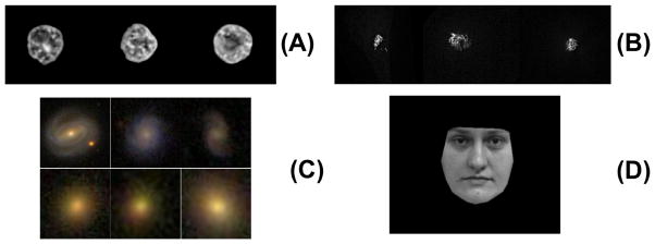
Sample images for the two data sets. A: Sample images from the liver nuclear chromatin data set. B: Sample images from the Golgi protein data set. C: Sample images from galaxy image data set. D: Sample image from facial expression data set.

5.2 Particle approximation error

Here we quantify how well our particle-based algorithm described above can approximate the different datasets we use in this paper. Instead of an absolute figure, of interest is the OT error between each image and its particle approximation, relative to the OT distances that are present in a dataset. Figure 7(A) can give us some indication of the relative (in percentage) error for the particle approximation of each image in each dataset. For each image in a dataset, we compute the error $e_i=\frac{{\varphi }_i}{\frac{1}{M}{\sum }_{j=1,\dots ,M}{d}_{i,j}}$, where d_i,j is the OT distance computed through equation (5), and ϕ_i is the upper bound on the OT distance between the particle approximation of image i and the image i (defined in equation (16) in the appendix). The computation is repeated for M images chosen randomly from a given dataset. Figure 7(A) contains the histogram of the errors for all the datasets. The x-axis represents the relative error in percentage, and the y-axis represents the portion of samples that has the corresponding relative error. Though, by definition, we can always reduce the approximation errors by adding more particles, considering the computational cost, we use 500 initial particles for the nuclei, golgi and galaxy data sets, and 2000 initial particles for the face data set. The data shows that the average errors were 14.1% for the nuclear chromatin dataset, 3.2% for the golgi protein dataset, 13.1% for the galaxy image dataset and 18.5% for the face data set.

Fig. 7.

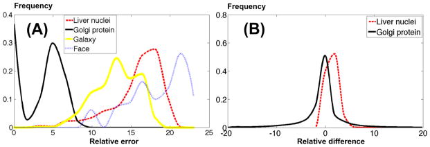
Histograms of particle approximation error and LOT error. A: The histogram of relative error generated during the particle approximation process. The x-axis represents the relative error in percentage, and the y-axis represents the portion of samples that has the corresponding relative error. B: The histogram of relative errors between LOT and OT for nuclei and golgi data sets. The x-axis represents the relative error in percentage, and the y-axis represents the portion of samples that has the corresponding relative error. The dotted line represents the relative errors for the liver nuclear chromatin dataset, and the solid line represents relative errors for the Golgi dataset.

5.3 Difference between OT and LOT

We compare the LOT distance given in equation (9) with the OT distance, defined in equation (5). To that end, we compute the full OT distance matrix (all pairwise distances) for both biological image datasets and compare it to the LOT distance via: $e_{OT,\mathit{LOT}}=\frac{d_{OT}-d_{\mathit{LOT}}}{d_{OT}}$. Figure 7(B) contains the relative error for the nuclear chromatin and golgi. The average absolute error for the nuclear chromatin data is e_OT,LOT = 2.94%, and e_OT,LOT = 3.28% for the golgi dataset.

5.4 Discrimination power

In [43], we have shown that the OT metric can be used to capture the nuclear morphological information to classify different classes of liver and thyroid cancers. We now show that the linear OT approximation we propose above can be used for discrimination purposes with little or no loss in accuracy when compared to traditional feature-based approaches. To test classification accuracy we use a standard implementation of the support vector machine method [7] with a radial basis function (RBF) kernel.

For the nuclear chromatin in the liver cancer dataset we followed the same leave one case out cross validation approach described in [43]. The classification results are listed in Table 1. For comparison, we also computed classification results using a numerical feature approach where the same 125 numerical features (including shape parameters, Haralick features, and multi-resolution-type features) as described in [43], were used. Stepwise discriminant analysis was used to select the significant features for classification (12 of them were consequently selected). In addition, we also provide classification accuracies utilizing the method described in [28], which we denote here as EMD-L1. The EMD-L1 in this case was applied to measure the L₁ weighted earth mover’s distance (EMD) between image pairs. The radius above which pixels displacements were not computed was set to 15 for fast computation. When using the EMD-L1 method, each image was downsampled by four, after Gaussian filtering, to allow for the computations to be performed in a reasonable time frame (see discussion section for a comparison and discussion of computation times).

Table 1.

Average classification accuracy in liver data

	Feature	OT	LOT	EMD-L1
Case 1	89%	87%	86%	84%
Case 2	92%	88%	89%	86%
Case 3	94%	91%	90%	87%
Case 4	80%	87%	85%	84%
Case 5	71%	76%	74%	76%
Average	85.2%	85.8%	84.8%	83.4%

Classification results are shown in Table 1. We note that because we used a kernel-based SVM method, the only difference between all implementations were the pairwise distances computed (OT vs. LOT vs. EMD-L1 vs. feature-based). In Table 1, each row corresponds to a test case, and the numbers correspond to the average classification accuracy (per nucleus) for normal liver and liver cancer. The first column contains the classification accuracy for the feature-based approach, the second column the accuracy for the OT metric, the third column the accuracy for the LOT metric, and the final column contains the computations utilizing the EMD-L1 approach [28]. We followed a similar approach for comparing classification accuracies in the golgi protein dataset. In this case we utilized the feature set described in [9]. This feature set was specifically designed for classification tasks of this type. A five fold cross validation strategy was used. Results are shown in Tables 2 and 3.

Table 2.

Average classification accuracy in golgi protein data

	Feature		OT		LOT
	gia	gpp	gia	gpp	gia	gpp
gia	79.2%	20.8%	86.2%	13.8%	83.8%	16.2%
gpp	28.6%	71.4%	35.6%	64.3%	30.7%	69.3%

Table 3.

Average classification accuracy for EMD-L1 in golgi protein data

	EMD-L1
	gia	gpp
gia	85.8%	14.2%
gpp	31.3%	68.7%

We also computed the LOT metric for the galaxy and facial expression datasets and applied the same support vector machine (SVM) strategy. In the galaxy case we utilized the feature set described in [34]. A five fold cross validation accuracy was used. Compared with the accuracy of the feature-based approach (93.6%), the classification accuracy of LOT metric was 87.7%. For the facial expression data set, the classification was performed based on SVM with the LOT metric, and a 90% classification accuracy was obtained.

5.5 Visualizing summarizing trends and discriminating information

We applied the PCA technique as described in section 4 to the nuclei and facial expression data sets. The first three modes of variation for the nuclear chromatin datasets (containing both normal and cancerous cells) are displayed in Figure 8(A). The first three modes of variation for the facial expression dataset are shown in Figure 8(B). For both datasets, the first three modes of variation correspond to over 99% of the variance of the data. The modes of variation are displayed from the mean to plus and minus four times times the standard deviation of each corresponding mode. For the chromatin dataset we can visually detect size (first mode), elongation (second mode), and differences in chromatin concentration, from the center to the periphery of the nucleus (third mode). In the face dataset, since we did not normalize for size of the face, one can detect variations in size (first mode), facial hair texture (second mode), as well as face shape (third mode). The variations detected from the second and third modes are similar to the results reported in [36].

Fig. 8.

The modes of variation given by the PCA method combined with the LOT framework, for nuclear chromatin (A) and facial expression (B) datasets. Each row corresponds to a mode of variation, starting from the first PCA mode (top).

We also applied the method described in Section 4 to visualize the most significant differences between the two classes in each dataset. The most discriminating modes for the nuclear chromatin dataset, golgi dataset, galaxy and the facial expression dataset are shown in Figure 9(A,B,C,D), respectively. In the nuclear chromatin case, the normal tissue cells tend to look more like the images on the left, while the cancerous ones tend to look more like the images on the right. In this case we can see that the most discriminating effect seems to be related to differences in chromatin placement (near periphery vs. concentrated at the center). The p value for this direction was 0.019. For the golgi protein dataset, the discriminating direction (p = 0.049) shows that the giantin golgi protein tends to be more scattered than the gpp protein, which tends to be more elongated in its spatial distribution. For the galaxy dataset, the discriminant direction (p = 0.021) seems to vary from a spiral structure to a bright dense disk. For the facial expression dataset, the discriminating direction (p = 0.011) shows a trend from a smiling face to a serious or neutral facial expression.

Fig. 9.

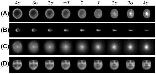
Modes of discrimination computed using the penalized LDA method in combination with the LOT framework. Each row contains the mode of variation that best discriminates the two classes in each dataset. Parts (A),(B),(C),(D) refer to discrimination modes in nuclear morphology, golgi proteins, galaxy morphology, and facial expression datasets, respectively.

6 Summary and Discussion

We described a new method for quantifying and visualizing morphological differences in a set of images. Our approach called the LOT is based on the optimal transportation framework with quadratic cost, and we utilize a linearized approximation based on a tangent space representation to make the method amenable to large datasets. Our current implementation is based on a discrete ‘particle’ approximation of each pattern, with subsequent linear programming optimization, and is therefore best suited for images which are sparse. We evaluated the efficacy of our methods in several aspects. As our results show, the error between an image and its particle approximation, relative to the distances in the dataset, are relatively small for a moderate number of particles when the images are sparse (e.g. golgi protein images), and can be made small for general images if more time is allowed for computation. We also showed that the LOT distance closely approximates the standard OT distance between particle measures, with absolute percentage errors on the order of a few percent in the datasets we used. In experiments not shown, we also evaluated the reproducibility of our particle-based LOT computation with respect to the random particle initializations required by algorithm. These experiments revealed that the average coefficient of variation was on the order of a couple of percent. Finally, we also evaluated how well the LOT distance described can perform in classifying sets of images in comparison to standard feature-based methods, the traditional OT distance [43], and the EMD-L1 method of [28]. Overall, considering all classification tests, no significant loss of accuracy was detected.

A major advantage of the LOT framework is the reduced cost of computing the LOT distance between all image pairs in a dataset. For a database of M images, section 2.3 explains that the number of transportation related optimization problems that need to be solved for computing all pairwise distances is M. In comparison, to our knowledge, the number of transportation related optimizations necessary for this purpose of all other available methods is M(M − 1)/2. In concrete terms, if all computations were to be performed using a single Apple laptop computer with 2GB or RAM and a dual processor of 2.2GHz, the total computation time for producing all pairwise distances for computing the results shown in Table 1 of our paper, for example, would be approximately 4.1 hours for the LOT method, 15.6 hours for the EMD-L1 method [28], and 1200 hours for the OT method described in [43]. We clarify that in order to utilize the EMD-L1 method images had to be downsampled to allow the computations to be performed in reasonable times. The time quoted above (and results shown in Tables 1, and 3) was computed by downsampling each image by a factor of four (after spatial filtering). We clarify again, however, that we have used a generic linear programming package for solving the OT optimizations associated with our LOT framework. The computation times for the LOT framework could be decreased further by utilizing linear programming techniques more suitable for this problem.

In addition to fast computation, a significant innovation of the LOT approach is the convenient isometric linear embedding it provides. In contrast to other methods that also obtain linear embeddings, see for example [31,37], the embedding LOT space allows for one to synthesize and visualize any point in the linear space as an image. Therefore the LOT embedding can facilitate visualization of the data distribution (via PCA) as well as differences between distributions (via penalized LDA). Hence, it allows for the automatic visualization of differences in both shape and texture in different classes of images. In biological applications, such meaningful visualizations can be important in helping elucidate effects and mechanisms automatically from the image data. For example, the results with the nuclear chromatin dataset suggest that, in this disease, cancer cells tend to have their chromatin more evenly spread (euchromatin) throughout the nucleus, whereas normal cells tend to have their chromatin in more compact form (heterochromatin). This suggests that the loss of heterochromatin is associated with the cancer phenotype in this disease. This finding is corroborated by earlier studies [42,43] (which used different methodology), as well as other literature which suggests that cancer progression is associated with loss of heterochromatin [25, 13].

We note that the use of the quadratic cost in (1) allows for a Riemannian geometric interpretation for the space of images. With this point of view, the LOT framework we describe can be viewed as a tangent plane approximation of the OT manifold. Thus the linear embedding we mentioned above can be viewed as a projection onto the tangent plane. While computing theoretical bounds for the difference between the OT and LOT distances is difficult since it would depend on the curvature of the OT manifold (which we have no way of estimating for a real distribution of images), several important facts about this approximation are worth noting. Firstly, we note that the LOT is a proper mathematical distance on its own, even when the tangent plane approximation is poor. Secondly, the projection is a one to one mapping. Thus information cannot be lost by projecting two images onto the same point. Finally, we note that utilizing the LOT distances (instead of the OT ones) results in no significant loss in classification accuracy. This suggests, that for these datasets, no evidence is available to prefer the OT space versus the LOT one.

As mentioned above, the LOT embedding obtained via the tangent space approximation can facilitate the application of geometric data analysis methods such as PCA to enable one to visualize interesting variations in texture and shape in the dataset. As compared to applying the PCA method directly on pixel intensities (data not shown for brevity), the PCA method applied with the use of the LOT method yields sharper and easier to interpret variations, since it can account for both texture and shape variations via the transportation of mass. As already noted above, several other graph-based methods also exist for the same purpose [31,37]. However, in contrast to our LOT method, these are not analytical meaning that only measured images can be visualized. Moreover, the LOT distances we provide here can be used as ‘local’ distances, based on which such graphs can be constructed. Thus both classes of methods could be used jointly, for even better performance (one example is provided in [30]).

The LOT framework presented here depends on a ‘particle’ approximation of the input images. The advantage of such a particle approximation is that the underlying OT optimization becomes a linear program whose global optimum can be solved exactly with standard methods. Drawbacks include the fact that such approach can become computationally intensive for non sparse images. We investigated the average classification accuracy for the experiments encountered in the previous section as a function of the number of particles used to approximate each image. For the experiment involving nuclear chromatin patterns, for example, the average classification accuracy for the LOT method using 300, 500, and 900 particles was 79%, 83.3%, and 83.4%, respectively. We note that for the golgi protein dataset, utilizing the LOT with 100 particles produced nearly the same accuracy as the ones reported in Table 2. These results, together with the already provided comparison to other methods, suggest the particle approximation was sufficient to classify these datasets.

Finally, we wish to point out several limitations inherent in the approach we describe here. First, as already noted, the particle approximation is best able to handle images which are sparse. For images that are not sparse, many more particles are needed to approximate the image well, thus increasing significantly the computational cost of the method. In addition, like all transportation related distances, our approach is not able to handle transport problems which include boundaries. Instead the approach is best suited for analyzing images whose intensities can be viewed as a distribution of mass that is ‘free’ to move about the image. In addition, we note that transportation-type distances are not good at telling the difference between smooth versus punctate patterns. For this specific task, other approaches (such as Fourier analysis, for example), may be more fruitful. Finally, we note that for some types of images, the traditional OT and the LOT can yield very different distances. This could occur when the images to be compared have very sharp transitions, of high frequency, and if the phase of these transitions are mismatched. We note that this is rarely the case in the images we analyze in this paper. These and other aspects of our current LOT framework will be the subject of future work.

Appendix: Particle approximation algorithm

Here we present the details of the particle approximation algorithm outlined in section 3.1. The goal of the algorithm is to approximate the given probability measure, μ on Ω by a particle measure with approximately N particles, where N is given. For images where the estimated error of the initial approximation is much larger than the typical error over the given dataset the number of particles is increased to reduce the error, while for images where the error is much smaller than typical the number of particles is reduced in order to save time when computing the OT distance. The precise criterion and implementation of adjusting the number of particles is described in step 8 below.

In our application the measure μ represents the image. It too can be thought as a particle measure particle measure itself $\mu ={\sum }_{j=1}^{N_{\mu }}{m}_j{\delta }_{y_j}$ where N_μ is the number of pixels, y_j the coordinates of the pixel centers, and m_j the intensity values. Our goal however is to approximate it with a particle measure with a lot fewer particles. Below we use the fact that the restriction of the measure μ to a set V is defined as $\mu {\mid }_V={\sum }_{i=1,x_i\in V}^{N_{\mu }}{m}_i{\delta }_{x_i}$. The backbone of the algorithm rests on the following mathematical observations.

Observation 1. The best approximation for fixed particle locations

Assume that x₁, …, x_N are fixed. Consider the Voronoi diagram with centers x₁, …, x_N. Let V_i be the cell of the Voronoi diagram that correspond to the center x_i. Then among all probability measures of the form $\mu ={\sum }_{i=1}^N{m}_i{\delta }_{x_i}$ the one that approximates μ the best is

$$\sum _{i=1}^N\mu (V_i){\delta }_{x_i}=\text{argmin}\left\{d_W(\mu ,{\mu }_N):{\mu }_N=\sum _{i=1}^N{m}_i{\delta }_{x_i}\text{with}{m}_i\ge 0\text{and}\sum _{i=1}^N{m}_i=\mu (\mathrm{\Omega })\right\}$$ (14)

Let us remark that if μ is a particle measure as above then μ(V_i) is just the sum of intensities of all pixels whose centers lie in V_i.

Given a measure μ supported on Ω we define the center of mass to be

$$x(\mu )=\frac{1}{\mu (\mathrm{\Omega })}{\int }_{\mathrm{\Omega }}xd\mu .$$ (15)

Observation 2. The best local ‘recentering’ of particles

It is easy to prove that among all one-particle measures the one that approximates μ the best is the one set at the center of mass of μ:

$$\mu (\mathrm{\Omega }){\delta }_{x(\mu )}=\text{argmin}\{d_W(\mu ,\mu (\mathrm{\Omega }){\delta }_y):y\in {\mathbb{R}}^n\}.$$

We can apply this to ‘recenter’ the delta measures in each Voronoi cell:

$$\sum _{i=1}^N\mu (V_i){\delta }_{x(V_i)}=\text{argmin}\left\{\sum _{i=1}^k{d}_W(\mu {{\mid }_V}_i,\mu (V_i){\delta }_{y_i}):y_i\in {\mathbb{R}}^n\right\}$$

Here μ|V_i is the restriction of measure μ to the set V_i. More precisely, for A ⊂ Ω, μ|V_i(A) = μ(A ∩ V_i).

Observation 3. The error for the current approximation is easy to estimate

Given a particle approximation as above one can compute a good upper bound on the error. In particular

$$\begin{array}{l}{d}_W^2\left(\mu ,\sum _{i=1}^N\mu (V_i){\delta }_{x(V_i)}\right)\le \sum _{i=1}^N{d}_W^2\left(\mu {\mid }_{V_i},\mu (V_i){\delta }_{x(V_i)}\right)\\ =\sum _{i=1}^N\int {\mid x-x(\mu {\mid }_{V_i})\mid }^{2}d\mu {\mid }_{V_i}.\end{array}$$ (16)

If $\mu ={\sum }_{j=1}^{N_{\mu }}{m}_j{\delta }_{y_j}$ the upper bound on the right-hand side becomes ${\sum }_{i=1}^N{\sum }_{j=1,y_j\in V_i}^{N_{\mu }}{m}_j{\mid y_j-{\overline{x}}_i\mid }^2$ where ${\overline{x}}_i=\left({\sum }_{j=1,y_j\in V_i}^{N_{\mu }}{m}_j{y}_j\right)/{\sum }_{j=1,y_j\in V_i}^{N_{\mu }}{m}_j$. We should also note that the estimate on the right-hand side gives us very useful information on ‘local’ error in each cell V_i. This enables us to determine which cells need to be refined when needed.

Based on these observations, we use the following ‘weighted Lloyd’ algorithm to produce a particle approximation to measure μ. The idea is to use enough particles to approximate each image well (according to the transport criterion), but not more than necessary given a chosen accuracy. The steps of our algorithm are:

1. Distribute N particles (with N an arbitrarily chosen number), x₁, … x_N, over the domain Ω by weighted random sampling (without replacement) the measure μ with respect to the intensity values of the image.

2. Compute the Voronoi diagram for centers x_i, …, x_k. Based on Observation 1, set m_i = μ(V_i). The measure ${\mu }_N={\sum }_{i=1}^N\mu (V_i){\delta }_{x_i}$ is the current approximation.

3. Using Observation 2, we recenter the cells by setting x_i,new = x(μ|V_i) (the center of mass of μ restricted to cell V_i).

4. Repeat steps 2. and 3. until the algorithm stabilizes. (the change of error upper bound is less than 0.5% in the sequential steps).

5. Repeat the steps 1 to 4 10 times for each image and choose the approximation with lowest error.

6. We then seek to improve the approximation in regions in the image which have not been well approximated by the step above. We do so by introducing more particles in the Voronoi cells V_i where the cost of transporting the intensities in that cell to its center of mass exceed a certain threshold. To do so, we compute the transportation error err_i = d_W(μ|V_i, μ(V_i)δ_xi) in cell i. Let err be the average transportation error. We add particles to all cells where err_i > 1.7err. More precisely if there are any cells where err_i > 1.7err then we split the cell with the largest error into two cells V_i1, V_i2, and then recompute the Voronoi diagram to determine the centers m_i1 = μ(V_i1), m_i2 = μ(V_i2) of these two new cells. We repeat this splitting process until all the Voronoi cells have error less than 1.7err_i. The choice of 1.7 was based on emperical evaluation with several datasets.

7. In order to reduce the number of particles in areas in each image where many particles are not needed, we merge nearby particles. Two particles are merged if, by merging them, the theoretical upper bound defined in (16) is lowered. When particles of mass m₁ and m₂ and locations x₁ and x₂ are merged to a single particle of mass m = m₁ + m₂ located at the center of mass $x=\frac{m_1{x}_1+m_2{x}_2}{m_1+m_2}$ the error in the m₁+m₂ distance squared is bounded by:

   $$d_W^2(m_1{\delta }_{x_1}+m_2{\delta }_{x_2}+{\mu }_{\mathit{rest}},m{\delta }_x+{\mu }_{\mathit{rest}})\le \frac{m_1{m}_2}{m_1+m_2}{\mid x_1-x_2\mid }^2$$

   We merge the particles that add the smallest error first and then continue merging until d_W(μ_N, μ_merged) < 0.15d_W(μ_N, μ). This has the overall effect of shifting the histogram (taken over all images) of the approximation error to the right, where the inequality is used in the sense of the available upper bound on the distance (Observation 3 and the estimate above) and not the actual distance. This ensures that the final error for each image after merging is around 1.15d_W(μ_N, μ).

8. Finally, while the two steps above seek to find a good particle approximation for each image, with N particles or more, the final step is designed to make the particle approximation error more uniform for all images in a given dataset. For a set of images I₁, I₂, …, I_M, we estimate the average transportation error, E_avg, between each digital image and its approximation, as well as standard deviation t of the errors. We set E_small = E_avg − 0.5 * τ and E_big = E_avg + 0.5 * τ.

   • For images that have bigger error than E_big, we split the particles as in Step 6 until the error for those images are less than E_big.

   • For images that have smaller error than E_small, we merge nearby particles instead as in Step 7. The procedure we apply is to merge the particles that add the smallest error first and then continue merging until d_W (μ, μ_merged) = E_small.

References

- 1.Ambrosio L, Gigli N, Savaré G. Lectures in Mathematics ETH Zürich. 2. Birkhäuser Verlag; Basel: 2008. Gradient flows in metric spaces and in the space of probability measures. [Google Scholar]
- 2.Angenent S, Haker S, Tannenbaum A. Minimizing flows for the Monge-Kantorovich problem. SIAM J Math Anal. 2003;35(1):61–97. (electronic) [Google Scholar]
- 3.Barrett JW, Prigozhin L. Partial L1 Monge-Kantorovich problem: variational formulation and numerical approximation. Interfaces Free Bound. 2009;11(2):201–238. [Google Scholar]
- 4.Beg M, Miller M, Trouvé A, Younes L. Computing large deformation metric mappings via geodesic flows of diffeomorphisms. International Journal of Computer Vision. 2005;61(2):139–157. [Google Scholar]
- 5.Benamou JD, Brenier Y. A computational fluid mechanics solution to the Monge-Kantorovich mass transfer problem. Numer Math. 2000;84(3):375–393. [Google Scholar]
- 6.Bengtsson E. Fifty years of attempts to automate screening for cervical cancer. Med Imaging Tech. 1999;17:203–210. [Google Scholar]
- 7.Bishop CM. Pattern Recognition and Machine Learning (Information Science and Statistics) Springer; 2006. [Google Scholar]
- 8.Blum H, et al. A transformation for extracting new descriptors of shape. Models for the perception of speech and visual form. 1967;19(5):362–380. [Google Scholar]
- 9.Boland MV, Murphy RF. A neural network classifier capable of recognizing the patterns of all major subcellular structures in fluorescence microscope images of hela cells. Bioinformatics. 2001;17(12):1213–23. doi: 10.1093/bioinformatics/17.12.1213. [DOI] [PubMed] [Google Scholar]
- 10.do Carmo MP. Mathematics: Theory & Applications. Birkhäuser Boston Inc; Boston, MA: 1992. Riemannian geometry. Translated from the second Portuguese edition by Francis Flaherty. [Google Scholar]
- 11.Chefd’hotel C, Bousquet G. Intensity-based image registration using earth mover’s distance. Proceedings of SPIE; 2007. p. 65122B. [Google Scholar]
- 12.Delzanno GL, Finn JM. Generalized Monge-Kantorovich optimization for grid generation and adaptation in Lp. SIAM J Sci Comput. 2010;32(6):3524–3547. [Google Scholar]
- 13.Dialynas GK, Vitalini MW, Wallrath LL. Linking heterochromatin protein 1 (hp1) to cancer progression. Mutat Res. 2008;647(1–2):13–20. doi: 10.1016/j.mrfmmm.2008.09.007. [DOI] [PMC free article] [PubMed] [Google Scholar]
- 14.Fisher RA. The use of multiple measurements in taxonomic problems. Annals of Eugenics. 1936;7:179–188. [Google Scholar]
- 15.Gardner M, Sprague B, Pearson C, Cosgrove B, Bicek A, Bloom K, Salmon E, Odde D. Model convolution: A computational approach to digital image interpretation. Cellular and molecular bioengineering. 2010;3(2):163–170. doi: 10.1007/s12195-010-0101-7. [DOI] [PMC free article] [PubMed] [Google Scholar]
- 16.Grauman K, Darrell T. Fast contour matching using approximate earth mover’s distance. Proceedings of the 2004 IEEE Computer Society Conference on Computer Vision and Pattern Recognition, CVPR; 2004; 2004. [Google Scholar]
- 17.Haber E, Rehman T, Tannenbaum A. An efficient numerical method for the solution of the L2 optimal mass transfer problem. SIAM J Sci Comput. 2010;32(1):197–211. doi: 10.1137/080730238. [DOI] [PMC free article] [PubMed] [Google Scholar]
- 18.Haker S, Zhu L, Tennenbaum A, Angenent S. Optimal mass transport for registration and warping. Intern J Comp Vis. 2004;60(3):225–240. [Google Scholar]
- 19.Kong J, Sertel O, Shimada H, BOyer KL, Saltz JH, Gurcan MN. Computer-aided evaluation of neuroblastoma on whole slide histology images: classifying grade of neuroblastic differentiation. Pattern Recognition. 2009;42:1080–1092. doi: 10.1016/j.patcog.2008.10.035. [DOI] [PMC free article] [PubMed] [Google Scholar]
- 20.Ling H, Okada K. An efficient earth mover’s distance algorithm for robust histogram comparison. IEEE Transactions on Pattern Analysis and Machine Intelligence. 2007:840–853. doi: 10.1109/TPAMI.2007.1058. [DOI] [PubMed] [Google Scholar]
- 21.Lloyd SP. Least squares quantization in pcm. IEEE Trans Inf Theory. 1982;28(2):129–137. [Google Scholar]
- 22.Loo L, Wu L, Altschuler S. Image-based multivariate profiling of drug responses from single cells. Nature Methods. 2007;4(5):445–454. doi: 10.1038/nmeth1032. [DOI] [PubMed] [Google Scholar]
- 23.Methora S. On the implementation of a primal-dual interior point method. SIAM Journal on Scientific and Statistical Computing. 1992;2:575–601. [Google Scholar]
- 24.Miller MI, Priebe CE, Qiu A, Fischl B, Kolasny A, Brown T, Park Y, Ratnanather JT, Busa E, Jovicich J, Yu P, Dickerson BC, Buckner RL. Collaborative computational anatomy: an mri morphometry study of the human brain via diffeomorphic metric mapping. Hum Brain Mapp. 2009;30(7):2132–41. doi: 10.1002/hbm.20655. [DOI] [PMC free article] [PubMed] [Google Scholar]
- 25.Moss TJ, Wallrath LL. Connections between epigenetic gene silencing and human disease. Mutat Res. 2007;618(1–2):163–74. doi: 10.1016/j.mrfmmm.2006.05.038. [DOI] [PMC free article] [PubMed] [Google Scholar]
- 26.Orlin JB. A faster strongly polynomial minimum cost flow algorithm. Operations Research. 1993;41(2):338–350. [Google Scholar]
- 27.Pele O, Werman M. A linear time histogram metric for improved sift matching. ECCV; 2008. [Google Scholar]
- 28.Pele O, Werman M. Fast and robust earth mover’s distances. Computer Vision, 2009 IEEE 12th International Conference on; IEEE. 2009. pp. 460–467. [Google Scholar]
- 29.Pincus Z, Theriot JA. Comparison of quantitative methods for cell-shape analysis. J Microsc. 2007;227(Pt 2):140–156. doi: 10.1111/j.1365-2818.2007.01799.x. [DOI] [PubMed] [Google Scholar]
- 30.Rohde GK, Ribeiro AJS, Dahl KN, Murphy RF. Deformation-based nuclear morphometry: capturing nuclear shape variation in hela cells. Cytometry A. 2008;73(4):341–50. doi: 10.1002/cyto.a.20506. [DOI] [PubMed] [Google Scholar]
- 31.Roweis ST, Saul LK. Nonlinear dimensionality reduction by locally linear embedding. Science. 2000;290(5500):2323–2326. doi: 10.1126/science.290.5500.2323. [DOI] [PubMed] [Google Scholar]
- 32.Rubner Y, Tomassi C, Guibas LJ. The earth mover’s distance as a metric for image retrieval. Intern J Comp Vis. 2000;40(2):99–121. [Google Scholar]
- 33.Rueckert D, Frangi AF, Schnabel JA. Automatic construction of 3-d statistical deformation models of the brain using nonrigid registration. IEEE Trans Med Imag. 2003;22(8):1014–1025. doi: 10.1109/TMI.2003.815865. [DOI] [PubMed] [Google Scholar]
- 34.Shamir L. Monthly Notices of the Royal Astronomical Society. 2009. Automatic morphological classification of galaxy images. [DOI] [PMC free article] [PubMed] [Google Scholar]
- 35.Shirdhonkar S, Jacobs D. Approximate earth mover’s distance in linear time. Proceedings of the 2008 IEEE Computer Society Conference on Computer Vision and Pattern Recognition, CVPR; 2008; 2008. [Google Scholar]
- 36.Stegmann M, Ersboll B, Larsen R. Fame-a flexible appearance modeling environment. IEEE Transactions on Medical Imaging. 2003;22(10):1319–1331. doi: 10.1109/tmi.2003.817780. [DOI] [PubMed] [Google Scholar]
- 37.Tenenbaum JB, de Silva V, Langford JC. A global geometric framework for nonlinear dimensionality reduction. Science. 2000;290(5500):2319–2323. doi: 10.1126/science.290.5500.2319. [DOI] [PubMed] [Google Scholar]
- 38.Vaillant M, Miller M, Younes L, Trouvé A. Statistics on diffeomorphisms via tangent space representations. NeuroImage. 2004;23:S161–S169. doi: 10.1016/j.neuroimage.2004.07.023. [DOI] [PubMed] [Google Scholar]
- 39.Villani C. Graduate Studies in Mathematics. Vol. 58. American Mathematical Society; Providence, RI: 2003. Topics in optimal transportation. [Google Scholar]
- 40.Villani C. Optimal transport, Grundlehren der Mathematischen Wissenschaften [Fundamental Principles of Mathematical Sciences] Vol. 338. Springer-Verlag; Berlin: 2009. URL http://dx.doi.org/10.1007/978-3-540-71050-9. Old and new. [DOI] [Google Scholar]
- 41.Wang W, Mo Y, Ozolek JA, Rohde GK. Penalized fisher discriminant analysis and its application to image-based morphometry. Pattern Recognition Letters. doi: 10.1016/j.patrec.2011.08.010. (accepted, 2011) [DOI] [PMC free article] [PubMed] [Google Scholar]
- 42.Wang W, Ozolek J, Rohde G. Detection and classification of thyroid follicular lesions based on nuclear structure from histopathology images. Cytometry Part A. 2010;77(5):485–494. doi: 10.1002/cyto.a.20853. [DOI] [PMC free article] [PubMed] [Google Scholar]
- 43.Wang W, Ozolek J, Slep cev D, Lee A, Chen C, Rohde G. An optimal transportation approach for nuclear structure-based pathology. IEEE Transactions on Medical Imaging. 2011;30(3):621–631. doi: 10.1109/TMI.2010.2089693. [DOI] [PMC free article] [PubMed] [Google Scholar]
- 44.Yang L, Chen W, Meer P, Salaru G, Goodell L, Berstis V, Foran D. Virtual microscopy and grid-enabled decision support for large scale analysis of imaged pathology specimens. IEEE Trans Inf Technol Biomed. 2009 doi: 10.1109/TITB.2009.2020159. [DOI] [PMC free article] [PubMed] [Google Scholar]