

Abstract
Estimation of genomic breeding values is the key step in genomic selection (GS). Many methods have been proposed for continuous traits, but methods for threshold traits are still scarce. Here we introduced threshold model to the framework of GS, and specifically, we extended the three Bayesian methods BayesA, BayesB and BayesCπ on the basis of threshold model for estimating genomic breeding values of threshold traits, and the extended methods are correspondingly termed BayesTA, BayesTB and BayesTCπ. Computing procedures of the three BayesT methods using Markov Chain Monte Carlo algorithm were derived. A simulation study was performed to investigate the benefit of the presented methods in accuracy with the genomic estimated breeding values (GEBVs) for threshold traits. Factors affecting the performance of the three BayesT methods were addressed. As expected, the three BayesT methods generally performed better than the corresponding normal Bayesian methods, in particular when the number of phenotypic categories was small. In the standard scenario (number of categories=2, incidence=30%, number of quantitative trait loci=50, h2=0.3), the accuracies were improved by 30.4%, 2.4%, and 5.7% points, respectively. In most scenarios, BayesTB and BayesTCπ generated similar accuracies and both performed better than BayesTA. In conclusion, our work proved that threshold model fits well for predicting GEBVs of threshold traits, and BayesTCπ is supposed to be the method of choice for GS of threshold traits.
Keywords: Bayesian methods, genomic selection, MCMC, threshold traits
Background
To overcome the problem with traditional marker-assisted selection (MAS) that only a limited proportion of the total genetic variance is captured by the markers, an alternative method termed genomic selection (GS) was presented by Meuwissen et al. (2001), which traces all quantitative trait loci (QTL) by tracing all chromosome segments through highly dense markers covering the whole genome. GS has become feasible very recently with the availability of high-throughput genotyping technology.
Estimation of genomic breeding values is the key step in GS, for which number of approaches have been proposed (Meuwissen et al., 2001; Zou and Hastie, 2005; Gianola et al., 2006; VanRaden, 2008; Yi and Xu, 2008; Solberg et al., 2009; Zhang et al., 2010; Habier et al., 2011). All of these methods focus on continuous traits. However, many traits of importance in animal production, such as littler size of large mammals, degree of calving difficulty and resistance to disease, present a discrete (or categorical) distribution of phenotypes, and are often termed threshold traits. Obviously, the GS methods proposed for continuous traits cannot be adequately applied for such kind of traits. Because outcomes of threshold traits are assigned into several mutually exclusive and exhaustive ordered categories, if they are processed as continuous ones by traditional linear model, issues are involved (Gianola, 1982, 1983), including (1) the relationship between variables and dependent phenotypes is non-linear; (2) phenotype observations do not follow normal distribution; (3) the variance is a function of the expectation. Therefore, threshold model, which relates a hypothetical underlying continuous scale to the outward phenotype, has been introduced for threshold traits analyses (Wright, 1934; Dempster and Lerner, 1950; Gianola, 1982, 1983; Albert and Chib, 1993; Sorensen et al., 1995; Falconer and Mackay, 1996; Sorensen, 2002; Zhang, 2007).
Here we introduce threshold model to the framework of GS and, specifically, we extend the three Bayesian methods (BayesA, BayesB and BayesCπ) for estimating the marker effects for threshold traits on the basis of the threshold model. The extended methods are correspondingly termed BayesTA, BayesTB and BayesTCπ. Computing procedures of the three BayesT methods using Markov Chain Monte Carlo (MCMC) algorithm are derived. A simulation study was performed to investigate the benefit of the presented methods in terms of accuracy with the genomic estimated breeding values (GEBVs) of threshold traits. In addition, we also applied our methods to the common data set from the fourteenth QTL–MAS workshop (Szydlowski and Paczyńska, 2011) to further confirm their feasibility. Factors affecting the three BayesT methods and their features were discussed.
Materials and methods
Models
Let l={li} (i=1, 2, …, n) be the vector of underlying latent variables or liabilities of all individuals. For the ith individual, it is postulated that
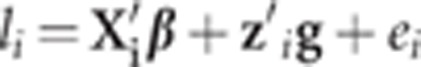 |
where β is the vector of location effects, g is the vector of single-nucleotide polymorphism (SNP) effects, ei is the random residual error with distribution of N(0, σ2e), x′i is the incidence row vector of β, z′i is the row vector of genotype indicators (with values 0, 1 or 2 for genotypes 11, 12 and 22, respectively). It is assumed that, given β and g, l is conditionally independent and distributed as
 |
As the liabilities are unobservable, the parameterization σ2e =1 will be adopted here, in order to achieve identifiability in the likelihood.
Let y={yi} (i=1,
2, …, n) denote the vector of observed categorical data. Here, each
yi represents an assignment into one of k
mutually exclusive and exhaustive categories. These classes result from the hypothetical
existence of k+1 thresholds in the latent scale, that is,
tmin<t1<t2<
…<tk−1<tmax
(tmin=−∞ and
tmax=∞). However, one of the thresholds must be fixed,
so as to center the distribution. A typical assignment is
t1=0. Then, the conditional probability that
yi falls in category j (j=1, 2,
…, k), given β, g and  , is given by
where Φ(•) is the cumulative distribution function of standard normal distribution. The data are conditionally independent, given β, g and t. Therefore, the sampling model can be written as
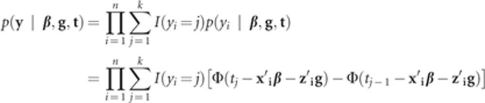 |
where I (yi=j) is an indicator function taking value of 1 if the response falls in category j and 0 otherwise.
MCMC implementation for BayesTA
Prior distribution and joint posterior density
It is assumed that each SNP has a different variance, and 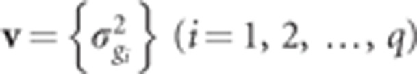 (i=1, 2, …,
q). In this study, the following prior distributions are chosen for
building a hierarchical model.
(i=1, 2, …,
q). In this study, the following prior distributions are chosen for
building a hierarchical model.
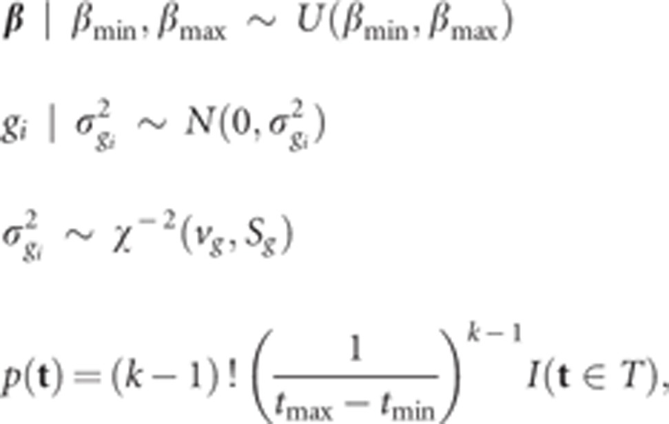 |
where 
The joint posterior distribution has a form of
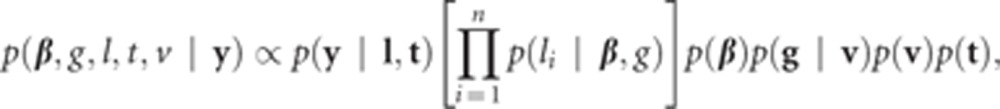 |
where 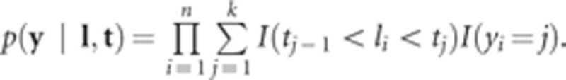 .
.
Fully conditional posterior distributions
Liabilities
The fully conditional posterior distribution of liability li is
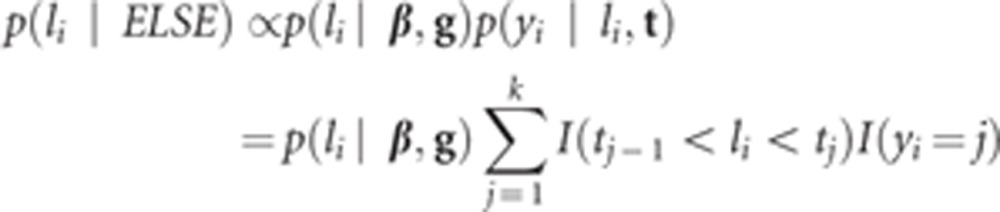 |
This is a truncated normal distribution, and its density is
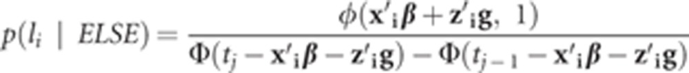 |
where φ (•) is the density function of standard normal distribution.
Thresholds
The density of the fully conditional posterior distribution of the jth threshold, tj, is
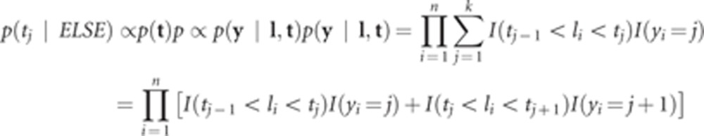 |
which shows that tj lies in an interval whose upper boundary must be smaller than or equal to the smallest value of l for which yi=j+1, and whose lower boundary is given by the maximum value of l for which yi=j. The prior condition (t∈T) is fulfilled automatically. Within these boundaries, the conditional posterior distribution of threshold tj is the uniform process
SNP effect variances
The fully conditional posterior distribution of the variance of the ith SNP effect, σ2gi, is
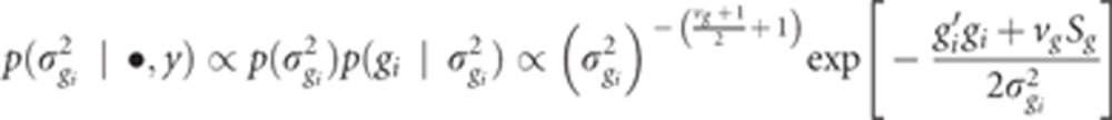 |
This is the kernel of the inverted χ2 distribution, therefore,
where  .
.
Location effects and SNP effects
The fully conditional posterior distribution of [β, g] is
Then
 |
where Xi is the ith column of X; β(i=0) equals β except that the value of βi is set to zero.
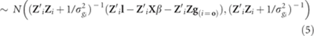 |
where Zi is the ith column of Z; g(i=0) equals g except that the value of gi is set to zero.
The Gibbs sampler
The Gibbs sampler consists of iterating through the following loop:
Sample the liabilities from the truncated normal distribution with density (1).
Sample the thresholds from the uniform distribution (2).
Sample the SNP effect variance from the scaled inverted χ 2 process (3).
Sample the location effects from the normal distributions (4).
Sample the SNP effects from the normal distributions (5).
Return to step 1 or terminate when chain length is adequate to meet convergence diagnostics.
MCMC implementation for BayesTB and BayesTCπ
Just as the three Bayesian methods (BayesA, BayesB and BayesCπ) for continuous traits, the differences between the three BayesT methods lay in the assumptions for the prior distribution of SNP effects. BayesTA assumes that all SNPs have an effect, but each has a different variance. BayesTB and BayesTCπ assume that each SNP has either an effect of zero or non-zero with probabilities π and 1-π, respectively, and for those having a non-zero effect, it is assumed that each SNP has a different variance in BayesTB and a common variance in BayesTCπ. In addition, in BayesTB π is treated as a known parameter, while in BayesTCπ it is treated as an unknown parameter with the prior distribution of uniform (0, 1). In this study, we set π=0.995 for BayesTB. Therefore, the MCMC Bayesian implementation procedure for BayesTA needs to be properly adjusted for BayesTB and BayesTCπ in the same way as for BayesB and BayesCπ (Meuwissen et al., 2001; Habier et al., 2011).
Simulation study
Data simulation
To evaluate the proposed methods, we simulated data for different scenarios.
The simulation started with a base population of 100 individuals, followed by 2000 non-overlapping historical generations with the same population size, denoted as generation −1999 to generation 0. In the base population and each historical generation, 50 males mated randomly with 50 females, and each mating produced two offspring (one male and one female). After the 2000 historical generations, six additional generations, numbered 1–6, were simulated. In generation 1, the population size was expanded from 100–1000 by randomly mating 50 males with 50 females in generation 0, and each mating produced 20 progenies (10 males and 10 females). From generation 1–5, 50 males were randomly selected from the 500 male individuals to be the sires of the next generation, and all 500 females were used as dams without selection. The population size of 1000 for generation 2–6 was obtained by randomly mating each male with 10 females and each female produced two offspring (one male and one female).
The simulated genome consisted of five chromosomes with a total length of 5 Morgan (1 Morgan per chromosome). On each chromosome, 2000 marker loci were randomly located and each segment between two markers was considered to harbor a potential QTL, giving 10 000 markers and 9995 potential QTL in total. For each true QTL, the allele substitution effect was drawn from the gamma distribution (1.66, 0.4). On the basis of the distance between two adjacent loci, Haldane's mapping function was used to calculate the probability of having a recombination between adjacent loci.
Genotypes and true breeding values were simulated for all individuals from generation 1–6, but phenotypic records of a discrete trait were only assigned to the 1000 individuals in generation 1 (training population).
In standard scenario, the following parameters were assigned: number of categories: 2 (binary trait with values 0 and 1), incidence: 30% (that is, 30% individuals having phenotypic value of 1), heritability of liability: 0.3, number of QTL: 50 (randomly selected from the 9995 putative QTL).
To investigate the effect of number of QTL, heritability, incidence and number of categories for the discrete trait, four groups of alternative scenarios were simulated in addition to the standard scenario described above. In the first group, three different levels of heritability were simulated: 0.05, 0.1 and 0.5. In the second group, different numbers of QTL were simulated: 20, 200 and 500. In the third group, different incidences of a binary trait were simulated: 5, 15 and 50%. In the fourth group, different numbers of trait categories were simulated: 3 (proportion of individuals in the three categories were 50%, 30%, 20%, respectively), 4 (proportion of individuals in the four categories were 30%, 40%, 20%, 10%, respectively), and 8 (proportion of individuals in the eight categories were 5%, 10%, 20%, 27%, 20%, 10%, 5%, 3%, respectively). For all these alternatives, only the relevant parameter was altered from the standard scenario. For all scenarios, 10 replicates were simulated.
Data from the fourteenth QTL–MAS workshop
The common data set of the fourteenth QTL–MAS workshop (Szydlowski and Paczyńska, 2011) consists of 3226 individuals from five consecutive generations (F0–F4). All individuals have genotypic records, while only 2326 individuals in generations F0–F3 have phenotypic records on two traits: a quantitative trait Q and a binary trait B. In this study, we only dealt with trait B. Individuals with phenotypic records (F0–F3) and without phenotypic records (F4) were treated as training and validation population, respectively. A genome consisting of 10 031 biallelic SNPs on five chromosomes with the length of 100 million bps each was simulated without any missing data and genotyping error.
Estimation of SNP effects
The three BayesT methods were used to estimate SNP effects in the training population. For comparison, BayesA, BayesB and BayesCπ were run on the same data, for which the discrete phenotypic values of threshold traits were treated as continuous ones. For all of the six Bayesian methods, the Markov chains were run for 20 000 cycles of Gibbs sampling (for BayesB and BayesTB, 100 additional cycles of Metropolis–Hastings sampling were performed for the SNP effect variance in each Gibbs sampling cycle), and the first 10 000 cycles were discarded as burn-in. All the samples of SNP effects after burn-in were averaged to obtain the SNP effect estimate.
For binary trait, Friedman et al. (2010) developed a computing program called GLMNET to estimate SNP effects, which fits a traditional logistic regression model with a lasso or elastic net regularization path by maximizing the appropriate penalized log-likelihood. Here, we compared the proposed Bayesian methods with GLMNET for the binary trait from both our simulation and the fourteenth QTL–MAS workshop. The tuning parameters for GLMNET were chosen by tenfold crossvalidation.
Calculation of GEBVs
GEBVs for individuals with genotypes, but no phenotypes, were calculated as the sum of all marker effects, according to their marker genotypes.
Results
Simulated data
Estimates of SNP effects in the standard scenario
Figure 1 shows the simulated QTL effects (Figure 1Q) and the SNP effects estimated by BayesA (Figure 1A), BayesB (Figure 1B), BayesCπ (Figure 1C), BayesTA (Figure 1TA), BayesTB (Figure 1TB), BayesTCπ (Figure 1tc) and GLMNET (Figure 1GLMNET) from a randomly selected replicate in the standard scenario (number of categories=2, incidence=30%, number of QTL=50, h2=0.3). While the simulated absolute QTL effects ranged from 0–0.61, the estimated absolute SNP effects ranged from 0–0.29 for BayesA and GLMNET, 0–0.13 for BayesB, BayesTA and BayesTB and 0–0.08 for BayesCπ and BayesTCπ. These estimated SNP effects, which were obviously not evenly distributed, reflected the underlying architecture of the trait. The estimated values of π were 0.998 and 0.994 for BayesCπ and BayesTCπ, respectively. Most segments containing big QTL were mapped by all methods.
Figure 1.

Simulated QTL effects and estimated SNP effects from a randomly selected replicate in the standard scenario (number of categories=2, incidence=30%, number of QTL=50, h2=0.3). Panel Q shows the absolute values of the simulated true QTL effects. Panels A, B, C, TA, TB, TC, and GLMNET show the absolute values of the SNP effects estimated by BayesA, BayesB, BayesCπ, BayesTA, BayesTB, BayesTCπ and GLMNET, respectively.
Accuracies of GEBVs in the standard scenario
Table 1 shows the accuracies of GEBVs in terms of correlations between GEBVs and simulated true breeding values in generation 2–6 in the standard scenario (number of categories=2, incidence=30%, number of QTL=50, h2=0.3). For all methods, the accuracies declined over generations with almost the same rate. Generally, the three BayesT methods (BayesTA, BayesTB and BayesTCπ) performed better than the corresponding normal Bayesian methods (BayesA, BayesB and BayesCπ) consistently in all generations. BayesA gave the lowest accuracies and BayesTA improved it dramatically. BayesTB and BayesTCπ yielded almost the same accuracies and their advantages over BayesB and BayesCπ were relatively small. In all generations, GLMNET generated accuracies lower than BayesTB and BayesTCπ, but higher than BayesTA.
Table 1. Accuracies of GEBVs obtained with the seven methods in generation 2–6 in the standard scenario (number of categories=2, incidence=30%, number of QTL=50, h 2=0.3).
| Method | Generation 2 | Generation 3 | Generation 4 | Generation 5 | Generation 6 |
|---|---|---|---|---|---|
| BayesA | 0.262±0.019 | 0.211±0.022 | 0.187±0.020 | 0.170±0.016 | 0.170±0.016 |
| BayesB | 0.671±0.029 | 0.624±0.031 | 0.597±0.035 | 0.570±0.039 | 0.570±0.038 |
| BayesCπ | 0.635±0.041 | 0.604±0.042 | 0.578±0.044 | 0.559±0.045 | 0.557±0.043 |
| BayesTA | 0.566±0.021 | 0.499±0.024 | 0.477±0.027 | 0.447±0.024 | 0.437±0.026 |
| BayesTB | 0.695±0.027 | 0.652±0.029 | 0.626±0.032 | 0.603±0.034 | 0.598±0.033 |
| BayesTCπ | 0.692±0.029 | 0.650±0.031 | 0.625±0.033 | 0.603±0.036 | 0.597±0.033 |
| GLMNET | 0.639±0.037 | 0.594±0.039 | 0.566±0.041 | 0.544±0.043 | 0.538±0.042 |
Abbreviations: GEBVs, genomic estimated breeding values; QTL, quantitative trait loci.
Values in the table are means and s.e.'s from 10 replicates.
In generation 2 in the standard scenario (number of categories=2, incidence=30%, number of QTL=50, h2=0.3), the average regression coefficients of true breeding values on GEBVs (measuring the biases of GEBVs) were 0.363, 4.110, 4.515, 0.347, 1.466, 1.671, 1.115 for BayesA, BayesB, BayesCπ, BayesTA, BayesTB, BayesTCπ and GLMNET, respectively.
Effect of heritability
Figure 2 shows the accuracies of GEBVs for different methods in generation 2 under different heritabilities. By decreasing the heritability from 0.5–0.05, the accuracies of all methods decreased as expected. In all cases, the three BayesT methods (BayesTA, BayesTB and BayesTCπ) performed better than the corresponding normal Bayesian methods (BayesA, BayesB and BayesCπ), and GLMNET yielded accuracies lower than BayesTB and BayesTCπ, but higher than BayesTA. However, when the heritability was low (0.05), the differences among BayesTB, BayesTCπ and GLMNET became bigger.
Figure 2.

Accuracies of GEBVs for different heritabilities (number of categories=2, incidence=30%, number of QTL=50). The graph shows the Pearson correlations between true breeding values (TBVs) and GEBVs estimated by BayesA, BayesB, BayesCπ, BayesTA, BayesTB, BayesTCπ and GLMNET in generation 2, while changing the heritability from 0.5–0.05.
Effect of number of QTL
As shown in Figure 3, BayesTB, BayesTCπ, BayesB, BayesCπ and GLMNET were sensitive to the number of QTL, and their accuracies decreased rapidly when the number of simulated QTL increased from 20–500. On the contrary, BayesTA and BayesA were not sensitive to the number of QTL, and their accuracies did not change with the number of simulated QTL.
Figure 3.

Accuracies of GEBVs for different number of QTL (number of categories=2, incidence=30%, h2=0.3). The graph shows the Pearson correlations between true breeding values (TBVs) and GEBVs estimated by BayesA, BayesB, BayesCπ, BayesTA, BayesTB, BayesTCπ and GLMNET in generation 2, while the number of simulated QTL increasing from 20–500.
The three BayesT methods performed better than the corresponding normal Bayesian methods in all cases except in the case of 20 QTL, where BayesB, BayesCπ, BayesTB and BayesTCπ gave almost the same accuracies. BayesTB and BayesTCπ almost obtained the same accuracies and their advantages over BayesB and BayesCπ increased along with the increase of the number of QTL. The advantages of BayesTA over BayesA were nearly stable in all cases. GLMNET generated lower accuracies than BayesTB and BayesTCπ in all cases except in the case of 20 QTL, where they performed almost equally well. The advantages of BayesTB, BayesTCπ and GLMNET over BayesTA declined rapidly with the increase of the number of simulated QTL, and in the case of 500 QTL, GLMNET lost its advantage over BayesTA.
Effect of incidence
Figure 4 shows the accuracies of GEBVs for different incidence of the binary trait. With the incidence decreasing from 50–5%, the accuracies of GEBVs declined consistently for all methods, but the three BayesT methods performed better than the corresponding normal Bayesian methods in all cases. BayesTB and BayesTCπ almost obtained the same accuracies, and their advantages over BayesB, BayesCπ and GLMNET increased with the decrease of the incidence.
Figure 4.

Accuracies of GEBVs for different incidence (number of categories=2, number of QTL=50, h2=0.3). The graph shows the Pearson correlations between true breeding values (TBVs) and GEBVs estimated by BayesA, BayesB, BayesCπ, BayesTA, BayesTB, BayesTCπ and GLMNET in generation 2, while the incidence decreasing from 50–5%.
Effect of number of phenotypic categories
As shown in Figure 5, with the increase of the number of phenotypic categories, the accuracies of GEBVs ascended for all the Bayesian methods, but the advantages of the three BayesT methods over the corresponding normal Bayesian methods decreased along with the increase of the number of categories. When the number of categories reached 8, the three BayesT methods completely lost their advantages. BayesTA was not sensitive to the number of categories, whereas BayesA was most sensitive among all methods.
Figure 5.

Accuracies of GEBVs for different number of phenotypic categories (number of QTL=50, h2=0.3). The graph shows the Pearson correlations between true breeding values (TBVs) and GEBVs estimated by BayesA, BayesB, BayesCπ, BayesTA, BayesTB and BayesTCπ in generation 2, while the number of phenotypic categories increasing from 2–8.
Common data set of the fourteenth QTL–MAS workshop
Using the seven methods, we analyzed the binary trait in the common data set of the fourteenth QTL–MAS workshop, for which 22 underlying QTL were simulated, and the incidence was 30% and heritability was 0.48 (Szydlowski and Paczyńska, 2011). For each Bayesian method, the analysis was repeated 10 times using different random seeds. The average estimated values of π were 0.997 for BayesCπ and 0.990 for BayesTCπ.
The accuracies and biases of GEBVs in the validation population are shown in Table 2. For this data set, the three BayesT methods gave better accuracies than the three corresponding normal Bayesian methods, respectively. The advantage was greater for BayesTA over BayesA, but smaller for BayesTB over BayesB, and BayesTCπ over BayesCπ. BayesTB and BayesTCπ yielded similar accuracies and were obviously better than GLMNET and BayesTA. All methods generated serious biases. However, in terms of the extent of biases, the three BayesT methods performed better than the three corresponding normal Bayesian methods, respectively.
Table 2. Accuracies and biases of GEBVs in the validation population of the common data set from the fourteenth QTL–MAS workshop.
| Method | Pearson's correlation | Regression coefficient |
|---|---|---|
| BayesA | 0.442±0.001 | 4.082±0.008 |
| BayesB | 0.816±0.007 | 17.790±0.184 |
| BayesCπ | 0.824±0.003 | 18.300±0.202 |
| BayesTA | 0.729±0.001 | 2.061±0.003 |
| BayesTB | 0.823±0.004 | 5.096±0.036 |
| BayesTCπ | 0.829±0.002 | 5.232±0.011 |
| GLMNET | 0.807 | 3.229 |
Abbreviations: GEBVs, genomic estimated breeding values; MAS, marker-assisted selection; QTL, quantitative trait loci.
Values for the Bayesian methods are means and s.e.'s from 10 runs with different random seeds.
Discussion
GS has revolutionized dairy cattle breeding by greatly increasing the accuracies of estimates of genetic merit for young animals and could double the rate of genetic progress by shortening the generation interval. To our knowledge, GS so far has focused on continuous traits. However, many threshold traits significantly affect profitability and are difficult to be selected. Therefore, GS for threshold traits is important in animal breeding.
As mentioned before, the estimation of genomic breeding values is the crucial step in GS. However, method for estimating genomic breeding values of threshold traits is scarce. Among many existing approaches for estimating genomic breeding values of quantitative traits, the three normal Bayesian methods (BayesA, BayesB and BayesCπ) are commonly used. But they are not suitable for threshold traits, because they are based on linear models.
Broadly speaking, the ideas of the three Bayesian methods (BayesA, BayesB and BayesCπ) were proposed long before the paper of Meuwissen et al., 2001. BayesA employs basically the same idea as the ridge-regression method (Hoerl and Kennard, 1970), because they shrink estimates with the L2 penalty. The difference between them is that the ridge regression assumes that all marker effects have a common variance, while BayesA allows each marker effect to have its own variance, and uses MCMC to generate the posterior sample of the parameters. This method has been used to map QTL under the random model by Xu (2003) and Wang et al. (2005), and many other people. They called it the Bayesian shrinkage method. BayesB is equivalent to the stochastic search variable selection method, which was originally developed by George and McCulloch (1993) and has been applied to QTL mapping by Yi et al. (2003) and Wang et al. (2005). BayesCπ is still the stochastic search variable selection method with variable π and has been used by Ishwaran and Rao (2005) (who named it the spike and slab variable selection) and Xu (2007). From these points of view, the three ‘BayesT' methods (BayesTA, BayesTB and BayesTCπ) proposed herein may also be regarded as threshold-model-versions of the Bayesian shrinkage method and the stochastic search variable selection method. Concurrent and independent work of threshold versions of BayesA and BayesB were reported very recently (González-Recio and Forni, 2011; Villanueva et al., 2011). However, no computing procedures were described therein. In our study, the MCMC computing procedures of the three BayesT methods were derived in detail and all fully conditional posterior distributions needed for running Gibbs sampling were given in closed forms, which will be helpful for later relevant studies. In addition, the factors (heritability, number of QTL, incidence, number of phenotype categories) affecting the performances of the three BayesT methods were systematically addressed. As expected, the three BayesT methods generally performed better than the corresponding normal Bayesian methods, particularly when the number of phenotypic categories was small. In the standard scenario (number of categories=2, incidence=30%, number of QTL=50, h2=0.3), the accuracies in generation 2 were improved by 30.4%, 2.4%, 5.7% points for BayesTA, BayesTB and BayesTCπ, respectively (Table 1).
In most cases, BayesTB and BayesTCπ generated similar accuracies of GEBVs despite their different assumptions on the prior distribution of marker effects, and performed much better than GLMNET and BayesTA, and GLMNET was better than BayesTA. From Figure 1, we can see BayesTB, BayesTCπ and GLMNET shrink the estimated effects of most SNPs toward zero via variable selection, whereas BayesTA gave non-zero estimates to all SNPs; so the higher accuracies resulted from reducing the noises. BayesB and BayesCπ performed fairly well for threshold trait, probably because they can apply variable selection to decrease the noises. In the standard scenario (number of categories=2, incidence=30%, number of QTL=50, h2=0.3) in generation 2, the accuracies of BayesTB and BayesTCπ were 5.6%, 5.3% points higher than that of GLMNET, respectively (Table 1).
Genetic architecture underlying the trait has significant effect on the performance of the methods. As shown in Figures 2 and 3, the accuracies of all methods declined with the decrease of the heritability or the increase of the number of QTL. Our results confirmed the observations for BayesB by Daetwyler et al. (2010). BayesTB, BayesTCπ, BayesB, BayesCπ and GLMNET are more sensitive to the variation of the number of QTL than BayesTA and BayesA. The advantages of BayesTB and BayesTCπ over BayesB and BayesCπ, respectively, declined rapidly with the decrease of the number of QTL, while the advantage of BayesTA over BayesA was nearly stable. When the number of QTL is very small (such as 20), BayesTB, BayesTCπ, BayesB, BayesCπ and GLMNET generate similar accuracies. That is partially confirmed by the results from the common data set of the fourteenth QTL–MAS workshop with only simulated 22 QTL for the binary trait (Szydlowski and Paczyńska, 2011). However, in real data, many quantitative traits and threshold traits are affected by large number of QTL with different effects (Goddard and Hayes, 2009), so the advantages of' using the BayesT methods for threshold traits should be considerable.
Phenotypic architecture of the trait also influences the performance of the methods. Figure 4 shows that with the incidence of a binary trait decreasing from 50–5%, the accuracies of GEBVs declined consistently for all methods. In particular, the decline was accelerated when the incidence was dropped from 15–5%. Even for BayesTB and BayesTCπ, which gave the highest accuracies in all incidences, the accuracy was only about 0.50 when the incidence was only 5%. Gilmour et al. (1985) suggested that if the overall incidence in the data is <30% or >70%, such data may not be informative for the estimation of variance components. For binary traits with low incidence (for example, <15%), very large training population is needed to achieve sufficient accuracies of GEBVs. As shown in Figure 5, for polychotomous traits, the advantages of the three BayesT methods over the corresponding normal Bayesian methods declined with the increase of the number of phenotypic categories. When the number of phenotypic categories reached 8, the three BayesT methods thoroughly lost their advantages. This again confirms that we can deal with the threshold traits with large number of phenotypic categories as continuous traits, but not for those with small number of phenotypic categories.
Conclusions
Our work proved that threshold model fits well for predicting GEBVs of threshold traits. In most scenarios, BayesTB and BayesTCπ generated similar accuracies and both performed better than GLMNET and BayesTA. However, it is not easy for BayesTB to choose a proper prior probability π that a SNP has a zero effect in real data. BayesTCπ addresses the drawback of BayesTA and BayesTB regarding the impact of prior hyperparameters and treats π as an unknown parameter to be estimated together with other parameters. Therefore, BayesTCπ is proposed as the method of choice for GS of threshold traits.
Data archiving
Data have been deposited at Dryad: doi:10.5061/dryad.pp551.
Acknowledgments
We thank the editor and the two referees for their useful comments. This work was supported by the ‘948' Project of the Ministry of Agriculture of China (Grant Number 2011-G2A), the PhD Programs Foundation of the Ministry of Education of China (Grant Number 20110008110001), the State High-Tech Development Plan of China (Grant Number 2011AA100302), the National Natural Science Foundation of China (Grant Number 30800776, 30972092, 31171200), Beijing Municipal Natural Science Foundation (Grant Number 6102016), the Modern Pig Industry Technology System Program of China and the Modern Pig Industry Technology System Program of Anhui Province.
The authors declare no conflict of interest.
References
- Albert JH, Chib S. Bayesian analysis of binary and polychotomous response data. J Am Stat Assoc. 1993;88:669–679. [Google Scholar]
- Daetwyler HD, Pong-Wong R, Villanueva B, Woolliams JA. The impact of genetic architecture on genome-wide evaluation methods. Genetics. 2010;185:1021–1031. doi: 10.1534/genetics.110.116855. [DOI] [PMC free article] [PubMed] [Google Scholar]
- Dempster ER, Lerner IM. Heritability of threshold characters. Genetics. 1950;35:212–236. doi: 10.1093/genetics/35.2.212. [DOI] [PMC free article] [PubMed] [Google Scholar]
- Falconer DS, Mackay TFC.1996Introduction to Quantitative Genetics4th edn.Longman: Essex, UK [Google Scholar]
- Friedman J, Hastie T, Tibshirani R. Regularization paths for generalized linear models via coordinate descent. J Stat Softw. 2010;33:1–22. [PMC free article] [PubMed] [Google Scholar]
- George EI, McCulloch RE. Variable selection via Gibbs sampling. J Am Stat Association. 1993;91:883–904. [Google Scholar]
- Gianola D. Theory and analysis of threshold characters. J Anim Sci. 1982;54:1079–1096. [Google Scholar]
- Gianola D, Foulicy JL. Sire evaluation for ordered categorical data with a threshold model. Genet Sel Evol. 1983;15:201–224. doi: 10.1186/1297-9686-15-2-201. [DOI] [PMC free article] [PubMed] [Google Scholar]
- Gianola D, Fernando RL, Stella A. Genomic-assisted prediction of genetic value with semiparametric procedures. Genetics. 2006;173:1761–1776. doi: 10.1534/genetics.105.049510. [DOI] [PMC free article] [PubMed] [Google Scholar]
- Gilmour AR, Anderson RD, Rae AL. The analysis of binomial data by a generalized linear mixed model. Biometrika. 1985;72:593–599. [Google Scholar]
- Goddard ME, Hayes BJ. Mapping genes for complex traits in domestic animals and their use in breeding programmes. Nat Rev Genet. 2009;10:381–391. doi: 10.1038/nrg2575. [DOI] [PubMed] [Google Scholar]
- González-Recio O, Forni S. Genome-wide prediction of discrete traits using Bayesian regressions and machine learning. Genet Sel Evol. 2011;43:7. doi: 10.1186/1297-9686-43-7. [DOI] [PMC free article] [PubMed] [Google Scholar]
- Habier D, Fernando RL, Kizilkaya K, Garrick DJ. Extension of the Bayesian alphabet for genomic selection. BMC Bioinformatics. 2011;12:186. doi: 10.1186/1471-2105-12-186. [DOI] [PMC free article] [PubMed] [Google Scholar]
- Hoerl AE, Kennard RW. Ridge regression: biased estimation for nonorthogonal problems. Technometrics. 1970;12:55–67. [Google Scholar]
- Ishwaran H, Rao JS. Spike and slab variable selection: frequentist and Bayesian strategies. Ann Stat. 2005;33:730–773. [Google Scholar]
- Meuwissen THE, Hayes BJ, Goddard ME. Prediction of total genetic value using genome-wide dense marker maps. Genetics. 2001;157:1819–1829. doi: 10.1093/genetics/157.4.1819. [DOI] [PMC free article] [PubMed] [Google Scholar]
- Solberg TR, Sonesson AK, Woolliams JA, Meuwissen THE. Reducing dimensionality for prediction of genome-wide breeding values. Genet Sel Evol. 2009;41:29. doi: 10.1186/1297-9686-41-29. [DOI] [PMC free article] [PubMed] [Google Scholar]
- Sorensen D, Andersen S, Gianola D, Korsgaard I. Bayesian inference in threshold models using Gibbs sampling. Genet Sel Evol. 1995;27:229–249. [Google Scholar]
- Sorensen D, Gianola D. Likelihood, Bayesian and MCMC Methods in Quantitative Genetics. Springer-Verlag: New York; 2002. [Google Scholar]
- Szydlowski M, Paczyńska P. QTLMAS 2010: simulated dataset. BMC Proc. 2011;5 ((Suppl 3)::S3. doi: 10.1186/1753-6561-5-S3-S3. [DOI] [PMC free article] [PubMed] [Google Scholar]
- VanRaden PM. Efficient methods to compute genomic predictions. J Dairy Sci. 2008;91:4414–4423. doi: 10.3168/jds.2007-0980. [DOI] [PubMed] [Google Scholar]
- Villanueva B, Fernández J, García-Cortés LA, Varona L, Daetwyler HD, Toro MA. Accuracy of genome-wide evaluation for disease resistance in aquaculture breeding programs. J Anim Sci. 2011;89:3433–3442. doi: 10.2527/jas.2010-3814. [DOI] [PubMed] [Google Scholar]
- Wang H, Zhang YM, Li X, Masinde GL, Mohan S, Baylink DJ, et al. Bayesian shrinkage estimation of quantitative trait loci parameters. Genetics. 2005;170:465–480. doi: 10.1534/genetics.104.039354. [DOI] [PMC free article] [PubMed] [Google Scholar]
- Wright S. An analysis of variability in number of digits in an inbred strain of Guinea Pigs. Genetics. 1934;19:506–536. doi: 10.1093/genetics/19.6.506. [DOI] [PMC free article] [PubMed] [Google Scholar]
- Xu S. Estimating polygenic effects using markers of the entire genome. Genetics. 2003;163:789–801. doi: 10.1093/genetics/163.2.789. [DOI] [PMC free article] [PubMed] [Google Scholar]
- Xu S. An empirical Bayes method for estimating epistatic effects of quantitative trait loci. Biometrics. 2007;63:513–521. doi: 10.1111/j.1541-0420.2006.00711.x. [DOI] [PubMed] [Google Scholar]
- Yi N, George V, Allison DB. Stochastic search variable selection for identifying quantitative trait loci. Genetics. 2003;164:1129–1138. doi: 10.1093/genetics/164.3.1129. [DOI] [PMC free article] [PubMed] [Google Scholar]
- Yi N, Xu S. Bayesian LASSO for quantitative trait loci mapping. Genetics. 2008;179:1045–1055. doi: 10.1534/genetics.107.085589. [DOI] [PMC free article] [PubMed] [Google Scholar]
- Zhang Q. Computational Methods in Animal Breeding. Science Press: Beijing; 2007. [Google Scholar]
- Zhang Z, Liu J, Ding X, Bijma P, de Koning D-J, Qin Z. Best linear unbiased prediction of genomic breeding values using a trait-specific marker-derived relationship matrix. PLoS ONE. 2010;5:e12648. doi: 10.1371/journal.pone.0012648. [DOI] [PMC free article] [PubMed] [Google Scholar]
- Zou H, Hastie T. Regularization and variable selection via the elastic net. J Royal Stat Soc B. 2005;67:301–320. [Google Scholar]