CLIP Test: a new fast, simple and powerful method to distinguish between linked or pleiotropic quantitative trait loci in linkage disequilibria analysis

Abstract

An important question arises when mapping quantitative trait loci (QTLs) for genetically correlated traits: is the correlation due to pleiotropy (a single QTL affecting more than one trait) and/or close linkage (different QTLs that are physically close to each other and influence the traits)? In this article, we propose the Close Linkage versus Pleiotropism (CLIP) test, a fast, simple and powerful method to distinguish between these two situations. The CLIP test is based on the comparison of the square of the observed correlation between a combination of apparent effects at the marker level to the minimal value it can take under the pleiotropic assumption. A simulation study was performed to estimate the power and alpha risk of the CLIP test and compare it to a test that evaluated whether the confidence intervals of the two QTLs overlapped or not (CI test). On average, the CLIP test showed a higher power (68%) to detect close-linked QTLs than the CI test (43%) and a same alpha risk (4%).

Introduction

Dense single nucleotide polymorphism (SNP) assays, now available for most species (human, livestock), make it possible to map quantitative trait loci (QTLs) using linkage disequilibrium (LD) between SNP markers and QTLs. Contrary to linkage analysis (LA), LD mapping does not require a specific family structure (Weller and Ron, 2011) and provides more accurate estimation of QTL positions (Meuwissen and Goddard, 2000). Many methods, from fast and simple (phenotype regression on marker genotypes; Long and Langley, 1999) to more complex but longer (random-effects models based on identity by descent matrix; Meuwissen and Goddard, 2000), have been proposed for mapping QTLs using LD or LDLA (Linkage Disequilibrium and Linkage Analysis). Generally, data relating to more than one trait are collected and, more often than not, these are correlated. Including information from all traits in a multiple-trait analysis has been reported to increase the power to detect QTLs in linkage experiments (Korol et al., 2001, Gilbert and Leroy, 2007) and association analysis (Ferreira and Purcell, 2009, Bolormaa et al., 2010). Mapping QTLs for genetically correlated traits leads to the following question: is the correlation due to pleiotropy (a single QTL affecting more than one trait) and/or close linkage (different QTLs that are physically close to each other and influence the traits; Falconer and Mackay, 1996)? If answering this question would provide information concerning the underlying mechanisms controlling the traits, it would also provide information about whether an unfavourable genetic correlation between two characters can be broken (in the case of linkage) or whether this is impossible (in the case of pleiotropism).

Several methods have been proposed to distinguish between linked and pleiotropic QTLs. Lebreton et al. (1998) proposed a bootstrap procedure in LA to reject the pleiotropic QTL hypothesis when confidence intervals for the difference between QTL locations did not include zero. Manichaikul et al. (2006), however, showed that the bootstrap procedure was not the most appropriate method when constructing confidence intervals for the locations of QTLs. Jiang and Zeng (1995) proposed a two-dimensional scan around the QTL position to test pleiotropy in a F2 population crossed from two inbred lines. In this region, flanking marker genotypes were used to calculate the test statistic based on the conditional probabilities of marker genotypes (Lander and Botstein, 1989). The test showed high power but the alpha risk was greater than the nominal level of 5% (that is, 10%). Knott and Haley (2000) proposed a similar procedure applied to a similar population using approximate likelihood ratio tests for multiple-trait least-squares analysis. These methods showed good performances but required successive multiple testing, and the null hypothesis test statistic distributions had to be generated that could be time-consuming when the number of SNP increases. Varona et al. (2004) presented a simple procedure, tested with LA, to calculate the Bayes factor between linked and pleiotropic QTL models. This procedure showed performances similar to those of the Knott and Haley method and did not require multiple testing. However, it used the MCMC (Markov chain Monte Carlo) method, which requires long computing times. All these methods were evaluated on data simulated for LA (F2, granddaughter design) analysed with a low density assay. It is therefore difficult to determine whether they might be valid in the case of LD analysis with complex pedigree structure and a high density chip. There are few specific methods reported in the literature that aim at distinguishing between linked and pleiotropic QTLs in the case of association analysis. Authors often conclude to patterns of pleiotropy if the same SNP or QTL region (determined subjectively (Mai et al., 2010) or using confidence interval (Tian et al., 2011)) affects both traits (Karasik et al., 2010, Olsen et al., 2011). Stich et al. (2008) assumed that discrimination between pleiotropy and close linkage of QTLs could be easily applied to the association analysis using a two-dimensional scan. Nevertheless, the performances of this test in such a situation have not been evaluated. Furthermore, conversely to LA, pleiotropic and close-linkage models are not nested in association analysis precluding the simple direct use of likelihood ratio -like tests. Indeed, the number of parameters are the same in the two models; these parameters are the effects of the same SNP for the two traits in the pleiotropic model and the effects of different SNP in the close-linked QTL model. Thus, one has to use parametric bootstrapping to obtain the significant threshold of the test, which is time consuming. Thomasen et al. (2008) compared pleiotropic and close-linkage models using the Bayesian Information Criteria (BIC; Schwarz, 1978); however, the BIC criterion is a tool for model selection and not for hypothesis testing (Pesaran and Weeks, 1999). Bolormaa et al. (2010) investigated pleiotropic effects by adjusting one trait with the other; thus removing almost all of the effect of that trait. The SNP in the highest LD with the pleiotropic QTL would then no longer have a significant effect on the adjusted trait. Nonetheless, this would also occur if the two SNPs, which are related to two close-linked QTLs, are in high LD.

None of the methods previously reported in the literature that aim at distinguishing between linked and pleiotropic QTLs considers the fact that, since the LD between a marker and the QTL is the same for the traits studied under the pleiotropic assumption, the pattern of the SNP effects (that is, the change in SNP effects when moving along the tested genomic region) should be similar for all of these traits, whereas it should be different under the close-linked QTL assumption. The Close Linkage versus Pleiotropism (CLIP) test that we propose here is based on this consideration.

The CLIP test aims at distinguishing between linkage or pleiotropy in a LD analysis with dense SNP assays whatever the complexity of the pedigree structure. First, the CLIP test is presented. Second, simulations are used to determine the power of detecting linked QTL and the risk of rejecting pleiotropic effects using the CLIP test in comparison with one of the most widely used method, which consists in testing whether the confidence intervals of the positions of the two QTLs overlap or not (CI test).

Materials and methods

Genetic model

Suppose N individuals, two phenotypes (y₁,y₂) per individual and two QTLs, QTL_k affecting the k^th trait (QTL₁=QTL₂ under the pleiotropism assumption). At the k^th QTL, there are three possible genotypes: Q_kQ_k, Q_kq_k and q_kq_k. The effects of these three genotypes on the quantitative trait are arbitrarily assigned the values a_k, d_k and −a_k, respectively, thus leading to the following model for the two phenotypic records of individual j:

where μ₁ and μ₂ are overall means, ξ_kj is the unobserved genotype for QTL_k and individual j, e_1j and e_2j are centred residuals, assumed to be normally distributed with the variance covariance matrix 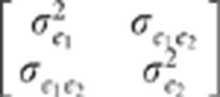. μ_1j and μ_2j are the effects of the background genes (polygenic effect) on traits 1 and 2, respectively. The density of the polygenic effects is assumed multivariate normal: , where A is the additive relationship matrix.

For the sake of simplicity, we first considered that traits were not under polygenic control or that the phenotypes had been pre-corrected for polygenic effects. The corresponding model (model 2) is then the same as model 1 removing the polygenic effects.

Suppose that a diallelic marker i is linked to the QTLs. We denoted the marker alleles as M and m. The ‘apparent effects' of the observed genotypes MM, Mm and mm at marker i are the means of the observed phenotypes of individuals being MM, Mm and mm at marker i, respectively. For each marker and each trait, we computed a linear combination of these apparent effects (Appendix 1 in Supplementary Material). The absolute value of the linear combination corresponds to half of the square root of the additive genetic variance calculated at the marker. Thus, the dataset containing these linear combinations was composed of 2n observations if there were n markers (one combination for each trait and each marker) instead of the 2N observations in the initial dataset. As the combination is function of the LD between the marker and the QTL, model (2) can be rewritten at the marker level (that is, considering the 2n combinations as the observations) as (Appendix 1 in Supplementary Material)

where X_1i and X_2i are combinations of the ‘apparent effects' of marker i on traits 1 and 2, respectively. where p_i denotes the marker i allele frequency and D_ki is the unobserved measure of LD between marker i and QTL_k (Hill and Robertson, 1968). Without lost of generality, we can assume that the that belong to [−1,1] are centred random variables. The parameters α and β are unknown. Their absolute values are the square root of the additive variance of QTL₁ and QTL₂ on traits 1 and 2, respectively, divided by 2pr₁(1−2pr₁) and 2pr₂(1−2pr₂), where pr_k denotes the allele frequency of QTL_k. S_1i and S_2i are normal random variables with a mean of 0. The variance covariance matrix of X₁,X₂ is denoted .

The CLIP test

Let us first give a flavour of the proposed method. When pleiotropism holds, for all markers i. In this case, model (3) shows that all the points are on the straight line defined by an intercept and a slope equal to 0 and , respectively. On the other hand when close linkage holds, for most of the markers i ( for a marker i is an exception). Therefore, the points are no longer on a straight line. Consequently, we would expect to observe an extra dispersion of Z_i around the straight line in the case of close linkage when compared with the pleiotropism situation. To illustrate that the points are not on a straight line under the close linkage assumption, we used the LD observed between markers reported by the Hapmap project (International HapMap Consortium (2003); 105 SNPs genotyped in the CEU population (Utah residents with Northern and Western European ancestry) on chromosome 9, in positions 700 000–800 000). We considered three sets of two adjacent markers with different LD values (RS7043585-RS4742292, r²=0.59; RS10815530-RS12685329, r²=0.87 and RS7849134-RS10739127, r²=1.00). 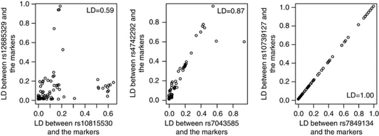We considered that these markers were QTLs and compared (as shown in Figure 1) the LD (r² which is proportional to between the QTLs and the remaining markers for the three sets of two adjacent QTLs. Figure 1 shows that, when r²=1.00 which is equivalent to the pleiotropism situation, are on a straight line. As soon as the LD falls below 1, are no longer on a straight line, even when the two SNPs are in high LD. Dispersion around the straight line increases when LD between QTLs decreases. The idea of the CLIP test is to compare the observed dispersion of Z_i around the straight line with the maximal dispersion that is expected in the pleiotropism situation. When the Z_i are more dispersed than expected, we conclude to close linkage. The correlation coefficient between X₁ and X₂ keeps track of this dispersion: a low correlation suggesting close linkage between QTLs and not pleiotropism.

Figure 1.

Change in the mean combination of apparent effects at the marker level for one trait as a function of the mean combination of apparent effects at the marker level for a second trait depending on the LD between the hypothetical QTLs for the two traits on chromosome 9 in position 700 000–800 000 of the human genome. The square of the mean combination of apparent effects at the marker level is expressed by the LD (r²) between the hypothetical QTLs and the remaining 105 markers. The two lefthand figures correspond to the hypothesis of close linkage, and the righthand figure corresponds to the hypothesis of pleiotropism. Under the pleiotropism assumption, points are on a straight line whereas they are not under the close linkage assumption. Dispersion around the straight line increases when the LD between QTLs decreases.

If is the observed correlation between and , their observed variances and the variances of the raw data, then the CLIP test consists of rejecting the hypothesis of pleiotropic QTLs when:

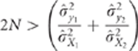and

where is the percentile of the distribution of the ratio of the square of the observed correlation to its minimal value under the pleiotropism assumption. The use of this multiplicative coefficient controls the risk of wrongly concluding linkage (alpha risk). The complete building of this test is provided in Appendix 2 in Supplementary Material. Thus, the CLIP test is composed of two inequalities. The first one is a necessary condition to ensure that the calculations performed in the second inequality make sense, that is, that the test can actually be performed. The second inequality corresponds to the comparison of the observed correlation to the minimal value it can take under the pleiotropism assumption. The term 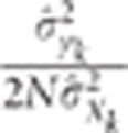is proportional to the inverse of the product of three terms, which are the relative importance of , and the variability of . Consequently, all things being equal, it is straightforward to acknowledge that the power of the CLIP test theoretically increases with QTL effects, with the variability of and with . We have demonstrated (Appendix 3 in Supplementary Material) that the CLIP test is consistent (that is, power of the test is 1 when grows to infinity). Unfortunately, the test's statistic is not parameter-free. Figure 2 shows how changes with using the approximation of the correlation coefficient distribution proposed by Chaubey and Mudholkar (1978). As changes with , it is difficult to choose a priori the value of which ensures a risk to wrongly reject the hypothesis of pleitropism of %. 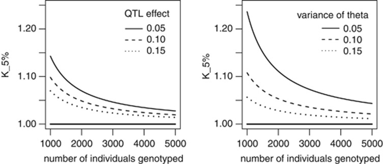Nonetheless, as it is shown in Figure 2, decreases monotonically to 1 with . Therefore, taking ensures the conservativeness of the CLIP test. Another possibility would be to obtain an estimation of to help in the choice of given the number of individuals genotyped.

Figure 2.

Changes in K_5% with the number of individuals genotyped depends on the QTL effect (left panel) and the variance of , the LD between the QTL and the markers (right panel). K_5% is always >1 and converges to 1 when the number of genotyped individuals increases. K_5% increases when the variance of the QTL effect and/or the variance of decreases

Simulation study

An analysis of simulated data, where the correct positions of the QTLs are known, was used to evaluate the proposed method. To investigate the performance of the CLIP test, data were generated under four simulation setups depending on the number of individuals genotyped (1365 or 2715) and the density of the SNP assay used (60 K or 800 K). Details of the simulation are provided in Table 1. It was assumed that a previous study had identified a small region, including two QTLs that affected the two traits. A QTL region of 0.1 (or 0.01) M containing 203 (or 263) equally spaced SNPs was then simulated to mimic 60 K (or 800 K) assay genotypes. Genotypes were simulated with the LDSO (Linkage Disequilibrium with Several Options) software (INRA, Jouy-en-Josas, France) (Ytournel et al., 2012). The initial SNP allele frequencies were drawn at random from a uniform distribution. There was no initial disequilibrium, that is, all alleles were present more than once in the population, and the alleles were attributed at random to each individual for each locus. LD between markers was created by two bottlenecks to mimic the LD observed at short distances in most species. The historical part of the simulated population consisted of 1030 generations of random mating in a population subjected to two changes in its size. The initial size of the population was 1000 individuals. The first change in its size happened at generation 501, reducing it from 1000 to 60 individuals. The second change happened at generation 1001, reducing it again from 60 to 30 individuals. Population size remained constant over the 30 last generations. The final population (the one genotyped and phenotyped) consisted of 1365 (or 2715) individuals across 5 generations (generations 1031–1035). Its pedigree structure was inspired from the one observed in livestock species; that is, complex pedigree with strong relationships between individuals. In the first generation, 15 sires were mated with 150 (or 300) dams (their parents were sampled from the historical part), each dam gave birth to two offspring with a sex ratio of 0.5. In all, 100% of the females and 10% of the males (randomly selected) were kept to be parents of the next generation. The QTL position and genotype for the first trait () were randomly sampled among the SNPs that had a minor allele frequency (MAF) >0.2. In the case of pleiotropy, the QTL position for the second trait () was the same as for the first trait. In the case of close linkage, the QTL position and genotype for the second trait were randomly sampled among the SNPs that were in the 0.5 cM region to the left of and the SNPs that were in the 0.5 cM region to the right of . If the MAF of proposed was <0.2 then the proposed QTL was rejected and another was sampled with the same acceptation rules. sampling was repeated until acceptance or at the most 40 times. If none of the 40 proposed was accepted, then a new population was simulated. Thus, when the two QTLs were in close linkage, the distance between the two QTLs varied from 0.05 to 0.5 cM for the 60 K assay and from 0.004 to 0.5 cM for the 800 K assay.

Table 1. Description of the simulated data.

Alternatives	Setups
	Number of individuals genotyped, density of the SNP assay
	1365 ind., 60 K; 2715 ind., 60 K; 1365 ind., 800 K; 2715 ind., 800 K
	0.4
	0.5
	−0.7,−0.3, 0, 0.3 or 0.7
	0.2
	0.3
	−0.7,−0.3, 0, 0.3 or 0.7
	0.07 or 0.1

Abbreviation: SNP, single nucleotide polymorphism.

Data were simulated according to model (1). : residual variance for trait : residual correlation between trait 1 and 2, ratio of the genetic variance to the residual variance for trait : genetic correlation between trait 1 and 2, ratio of the quantitative trait loci variance to the residual variance for trait k.

All individuals in the final population were genotyped and phenotyped. Phenotypes were generated according to model (1) considering that QTL effects were additive (that is, ).

For each individual, three phenotypes were simulated, a phenotype for the first trait, a phenotype for the second trait under the pleiotropic assumption and a phenotype for the second trait under the close linkage assumption. Residual variances were fixed to 0.4 and 0.5 for the first and second trait, respectively. Five correlations between residuals were considered, that is, −0.7, −0.3, 0, 0.3 and 0.7. Polygenic variances represented 20% and 30% of the corresponding residual variance for the first and second trait, respectively. Five correlations between polygenic effects of the two traits were considered, that is, −0.7, −0.3, 0, 0.3 and 0.7. The percentage of additive variance explained by the QTL took two possible values: 7% and 10% of the corresponding residual variance. Thus, there were 50 different alternatives for each simulation setup. For each simulation setup, 100 independent datasets were generated.

The data were analysed using two methods, the CLIP test and the CI test, the latter being the most widely used method in association analysis. Data were first corrected for the polygenic effects. To do so, data were analysed under the following mixed model:

Parameters were estimated using the restricted maximum likelihood. The residuals from this analysis were used as the dependent traits for the two tests. Only SNPs with a MAF >5% and which were not defined as a QTL were used for the analysis. The CLIP test was performed for all replicates and scenarios following the above described procedure and a fixed value of to ensure the conservativeness of the test. The principle of the CI test consisted of using cross-validation to calculate approximate 95% confidence intervals for the location of QTLs. The method was performed in two steps. We first evaluated if there was a significant SNP affecting each trait using simple linear regressions for each SNP and each trait. The SNP giving the minimal sums of squares was defined as the SNP being in strongest LD (closest) with the QTL. Correction for multiple testing was performed using the method proposed by Nyholt (2004). In the second step, the data was randomly split into two halves. The test of presence of QTL was then re-run for each half of the data and for each trait. When the significant SNP with the smallest sums of squares was detected close to the one detected in the full data set (<40 markers away () for the 60 K assay, <100 markers away () for the 800 K assay) for each trait and for each half of the data, the position of the corresponding SNP ( for the first and second half of the data, respectively, for trait , significant replicate l) was retained. The second step was repeated 500 times. The standard error of the position of QTL_k was calculated as: for L pairs (among the 500 replicates) of significant SNPs. The 95% confidence interval was then defined as the position of the most significant SNP from the full data analysis . Depending on whether the 95% confidence intervals for estimated positions of the two QTLs overlap or not, the test concludes to linkage or pleiotropy.

Results

The mean distance between the two QTL in the case of close-linked QTLs was 0.22 cM (±0.12) for the 60 K assay and 0.24 cM (±0.14) for the 800 K assay. The corresponding LD (r²) was 0.37 (±0.31) and 0.40 (±0.30) for the 60 K and 800 K assay, respectively. The mean number of SNPs used for the analysis (MAF>5%) was 90 (±16) for the 60 K SNP assay and 124 (±18) for the 800 K SNP assay.

For 2% of the simulated data sets, N was not large enough to satisfy the first inequality of the CLIP test. Likewise the CI test was not performed for 9% of the simulated data sets because no significant SNPs were detected for both the traits. Mean alpha risks and powers for the CLIP and CI tests, which depend on the experimental design (that is, density of the SNP assay, number of individuals genotyped), are presented in Table 2. The alpha risk was calculated as the percentage of simulations performed under the pleiotropic assumption for which the test was performed, and the null hypothesis of pleiotropism rejected. The mean alpha risk of the CLIP test was equal to 3% or 4% depending on the setup. The mean alpha risk of the CI test was equal to 6% for the 60 K assay and 2% for the 800 K assay. When data were simulated under the linked QTL assumption, the power of the tests was calculated as the proportion of times for which the test was performed, and the null hypothesis was rejected. The mean power to detect close-linked QTLs was 68% for the CLIP test and 43% for the CI test. For both the tests, power increased with the number of individuals genotyped (+19% and+12% for the CLIP and CI test, respectively). The power of the CLIP and CI tests increased with SNP density (+4% and+28% for the CLIP test and CI test, respectively).

Table 2. Mean power and alpha risk of the CLIP and CI tests depending on the setup.

Number of individuals	SNP density	Power		Alpha risk
		CLIP	CI	CLIP	CI
1365	60 K	57 (23)	25 (24)	4 (138)	6 (84)
	800 K	61 (27)	50 (16)	3 (157)	2 (105)
2715	60 K	75 (9)	34 (20)	4 (171)	6 (76)
	800 K	80 (11)	65 (13)	4 (136)	2 (97)

Abbreviations: CI, confidence interval; CLIP, close linkage versus pleiotropism; SNP, single nucleotide polymorphism.

RSD in bracket: relative standard deviation (in percentage) calculated over the different alternatives within each setup.

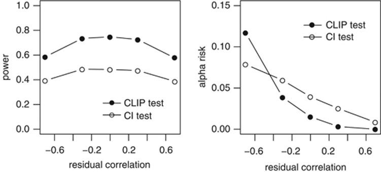
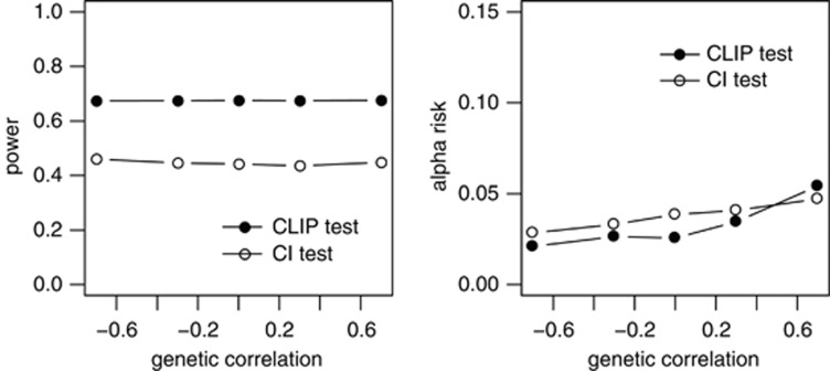
Changes in power and alpha risk due to the characteristics of the traits studied are presented below. The impacts of QTL effects on the power and alpha risks of the CLIP and CI tests are presented in Table 3. For both the tests, power increased with the QTL effect (+8 and +6% for the CLIP and CI tests, respectively), whereas the alpha risk was not affected by the effect of the QTL. The impact of residual correlations on the performances of the two tests is presented in Figure 3. The same pattern is observed for the two tests. There was no change in the power of either test due to change in the residual correlation within the [−0.3, 0.3] variation interval, but the power of the tests decreased when the absolute value of the correlation between residuals was high (0.7). For both tests, the alpha risk increased when residual correlation decreased. The alpha risk was found to be >5% for the CI test when residual correlation was negative. The alpha risk for the CLIP test was >5% when the residual correlation was equal to −0.7, and under 5% otherwise. The impact of genetic correlations on the performances of the two tests is presented in Figure 4. Once again, the same pattern is observed for the two tests. The changes in the genetic correlation had no effect on the power of the tests, whereas the alpha risk increased slightly when the genetic correlation increased. Nonetheless, the mean alpha risk was <5% for both the tests and all genetic correlation values.

Table 3. Impact of the size of the QTL effect on the power to detect close-linked QTLs and on the alpha risk to reject pleiotropic QTL for CLIP and CI tests.

CLIPPowerAlpha risk		64 (25)4 (153)	72 (18)4 (147)
CIPowerAlpha risk		40 (40)4 (104)	46 (38)4 (103)

Abbreviations: CI, confidence interval; CLIP, close linkage versus pleiotropism; QTL, quantitative trait loci.

: ratio of the QTL variance to the residual variance.

RSD in bracket: relative standard deviation (in percentage) calculated over the different alternatives and setup within each QTL effect group.

Figure 3.

CLIP and CI tests—impact of the residual correlation on the power to detect close-linked QTLs and on the alpha risk to reject pleiotropic QTLs. For both tests, power decreases when the absolute value of the residual correlation is high; alpha risk increases when the residual correlation decreases.

Figure 4.

CLIP and CI tests—impact of the genetic correlation on the power to detect close-linked QTL and on the alpha risk to reject pleiotropic QTLs. For both tests, there is no change in power with genetic correlation. The alpha risk increases slightly when the genetic correlation increases.

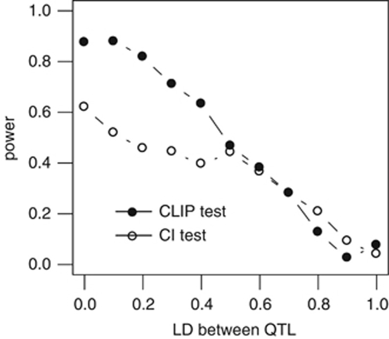
The variation of power with LD is presented in Figure 5. For both the tests, the power decreased when LD between QTLs increased. The decreases showed slightly different profiles for the two tests: the slope was steeper for the CLIP test than for the CI test, and the two curves crossed at a LD of approximately 0.5. The power of the CLIP test was then much higher than power of the CI test when values of LD between QTLs were <0.5.

Figure 5.

CLIP and CI tests—impact of LD between QTLs on the power to detect close-linked QTLs. For both tests, power decreases when the LD between the two QTLs increases. The power of the CLIP test is greater than the power of the CI test for a LD <0.5.

Discussion

The CLIP test uses information provided by close markers to distinguish linked versus pleiotropic QTL. The hypothesis tested by this test is that marker effects have the same pattern for the two traits in the case of pleiotropism (H0) but different patterns in the case of close linkage (H1). In the present study, the multiplicative coefficient was fixed to 1, thus providing a mean alpha risk <5%. Increasing would increase the alpha risk and the power of the CLIP test.

The CLIP test has the advantage over other methods of requiring only a single test, and is therefore much faster. Its calculation of means and correlations is instantaneous and furthermore its computing time does not increase a lot with the number of SNPs, contrary to all other methods based on multiple testing for SNPs that also require time-consuming methods to control the alpha risk (Churchill and Doerge, 1994).

In this article, the CLIP test has been described in the case where data have been previously corrected for polygenic effects. The test can also be performed without correction, and this could be an interesting application when pedigrees are not clearly established. This is another advantage of the CLIP test over other methods. In this case (no correction), if is the estimated mean relationship coefficient between individuals (that is, the sum of the relationship coefficients between individuals divided by the number of relationships), the CLIP test is the following (Appendix 4 in Supplementary Material):

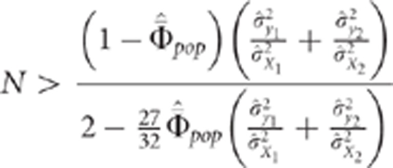This last equality confirms intuition and shows that must not be too large in order to be able to distinguish between the linked and pleiotropism situations. Pedigree structures in human populations should well fit this constraint.

Theoretically, extension of the CLIP test to more than two traits could be performed by studying the maximal volume of the dispersion of the points around the straight line under the pleiotropism assumption. Further work is needed to develop the CLIP test in such situations.

The results of the simulation study show that the CLIP test performs well compared with the CI test. The increase in power with SNP density, number of individuals genotyped and effect of the QTL is consistent with that reported in previous studies presenting other methods (Lebreton et al., 1998; Knott and Haley, 2000). The mean alpha risk for the CI test was <5% for the 800 K assay. This indicates that the size of the region we defined for accepting significant SNPs in the cross-validation procedure was too large for the 800 K assay and highlights the difficulties that exist as to the definition of this region. The variation of the power of the CLIP test with residual correlation showed that its power decreased when the absolute value of the correlation between residuals increased. An opposite pattern was reported by Lebreton et al. (1998) for the selective bootstrap procedure used for LA. Nonetheless, this observation was not consistent. Actually, these authors showed that the pattern of power variation changed depending on the importance of the QTL effect. In our case, the pattern was the same for the two sizes of QTL effect and for the two tests. The variation of the alpha risk with residual correlation showed that the alpha risk increased when residual correlation decreased. An opposite pattern would be observed if the QTL effects were simulated in the opposite direction. We showed that the alpha risks of both the CLIP and CI tests increased slightly with the genetic correlation. The changes in the performances of the tests with residual and genetic correlation are difficult to explain. They may not be directly related to the tests or to the initial data structure but rather to the pre-correction of the phenotypes for polygenic effects. In fact, Aulchenko et al. (2007) showed, using single trait analysis, that correction for polygenic effects tends to underestimate the SNP effect conversely to a method that uses restricted maximum likelihood to estimate parameters in model (1). This may explain why the two tests, which are not based on the same method, display the same change in performances with genetic and residual correlations. The decrease of the power of the CLIP test with LD demonstrates that when the LD is <0.7, the CLIP test performs similarly or even better than the CI test. As a LD >0.7 is rare even at short distances, this indicates that the CLIP test would perform better than the CI test for most cases of close-linked QTLs.

The CI test that we used as a reference test may not be the most powerful method. We performed the same simulation design using the non-parametric bootstrap test (Lebreton et al., 1998) adapted for association analysis to test linkage versus pleiotropy. The test showed performances similar to those of the CI test (average power of 46% and average alpha risk of 4%).

In practice, to perform the CLIP test, one has to choose the markers region to be considered. Ideally, this region must include markers that are in different LD with the QTL affecting the first trait and/or with the QTL affecting the second trait and in linkage equilibrium with other QTL. This region should be easy to identify using results of a genome-wide association study. Nonetheless, if a second close QTL region is suspected for almost one of the trait (trait 1 for instance); we recommend to evaluate the presence of two QTLs in the region using a Bayes Cπ (Habier et al., 2011) for instance. If the presence of two QTLs in the region is confirmed for trait 1, then the CLIP test should be performed on data corrected for the effect of this second QTL on trait 1 to prevent wrongly rejecting the hypothesis of pleiotropism.

To conclude, we have developed a fast, simple and powerful method, the CLIP test, to distinguish between linked or pleiotropic QTLs. The CLIP test is very easy to implement. It simultaneously uses information provided by several markers and has the advantage over other methods of not requiring multiple testing. We have demonstrated, by using simulations, that the power of the CLIP test is, on average, much higher than that obtained when comparing the confidence intervals of the two QTLs and that its alpha risk is lower. The CLIP test presented here has been used with data pre-corrected for polygenic effect but can be applied without such pre-correction. This would avoid bias and the decrease in performance due to the pre-correction.

Data archiving

The code of the simulation and of the CLIP test have been deposited at Dryad: doi:10.5061/dryad.m0584.

The authors declare no conflict of interest.

References

- Aulchenko YS, de Koning DJ, Haley C. Genomewide rapid association using mixed model and regression: a fast and simple method for genomewide pedigree-based quantitative trait loci association analysis. Genetics. 2007;177:577–585. doi: 10.1534/genetics.107.075614. [DOI] [PMC free article] [PubMed] [Google Scholar]
- Bolormaa S, Pryce JE, Hayes BJ, Goddard ME. Multivariate analysis of a genome-wide association study in dairy cattle. J Dairy Sci. 2010;93:3818–3833. doi: 10.3168/jds.2009-2980. [DOI] [PubMed] [Google Scholar]
- Chaubey YP, Mudholkar GS. A new approximation for Fisher's z. Aust J Stat. 1978;20:250–256. [Google Scholar]
- Churchill GA, Doerge RW. Empirical threshold values for quantitative trait mapping. Genetics. 1994;138:963–971. doi: 10.1093/genetics/138.3.963. [DOI] [PMC free article] [PubMed] [Google Scholar]
- Falconer DS, Mackay TFC.1996Introduction to quantitative genetics4th edn.Longman Group Essex, UK [Google Scholar]
- Ferreira MAR, Purcell SM. A multivariate test of association. Bioinformatics. 2009;25:132–133. doi: 10.1093/bioinformatics/btn563. [DOI] [PubMed] [Google Scholar]
- Gilbert H, Leroy P. Methods for the detection of multiple linked QTL applied to a mixture of full and half sib families. Genet Sel Evol. 2007;39:139–158. doi: 10.1186/1297-9686-39-2-139. [DOI] [PMC free article] [PubMed] [Google Scholar]
- Habier D, Fernando RL, Kizilkaya K, Garrick DJ. Extension of the bayesian alphabet for genomic selection. BMC Bioinformatics. 2011;12:186–198. doi: 10.1186/1471-2105-12-186. [DOI] [PMC free article] [PubMed] [Google Scholar]
- Hill WG, Robertson A. Linkage disequilibrium in finite populations. Theor Appl Genet. 1968;38:226–231. doi: 10.1007/BF01245622. [DOI] [PubMed] [Google Scholar]
- International HapMap Consortium The International HapMap Project. Nature. 2003;426:789–796. doi: 10.1038/nature02168. [DOI] [PubMed] [Google Scholar]
- Jiang C, Zeng Z. Mutiple trait analysis of genetic mapping for quantitative trait loci. Genetics. 1995;140:1111–1127. doi: 10.1093/genetics/140.3.1111. [DOI] [PMC free article] [PubMed] [Google Scholar]
- Karasik D, Hsu Y, Zhou Y, Cupples LA, Kiel DP, Demissie S. Genome-wide pleiotropy of osteoporosis-related phenotypes: the Framingham study. J Bone Min Res. 2010;25:1555–1563. doi: 10.1002/jbmr.38. [DOI] [PMC free article] [PubMed] [Google Scholar]
- Knott SA, Haley CS. Multitrait least squares for quantitative trait loci detection. Genetics. 2000;156:899–911. doi: 10.1093/genetics/156.2.899. [DOI] [PMC free article] [PubMed] [Google Scholar]
- Korol AB, Ronin YI, Itskovich AM, Peng J, Nevo E. Enhanced efficiency of quantitative trait loci mapping analysis based on multivariate complexes of quantitative traits. Genetics. 2001;157:1789–1803. doi: 10.1093/genetics/157.4.1789. [DOI] [PMC free article] [PubMed] [Google Scholar]
- Lander ES, Botstein D. Mapping mendelian factors underlying quantitative traits using RFLP linkage maps. Genetics. 1989;121:185–199. doi: 10.1093/genetics/121.1.185. [DOI] [PMC free article] [PubMed] [Google Scholar]
- Lebreton CM, Visscher PM, Haley CS, Semikhodskii A, Quarrie SA. A nonparametric bootstrap method for testing close linkage vs. pleiotropy of coincident quantitative trait loci. Genetics. 1998;150:931–943. doi: 10.1093/genetics/150.2.931. [DOI] [PMC free article] [PubMed] [Google Scholar]
- Long AD, Langley CH. The power of association studies to detect the contribution of candidate genetic loci to variation in complex traits. Genome Res. 1999;9:720–731. [PMC free article] [PubMed] [Google Scholar]
- Mai MD, Sahana G, Christiansen FB, Guldbrandtsen B. A genome-wide association study for milk production traits in Danish Jersey cattle using a 50 K single nucleotide polymorphism chip. J Anim Sci. 2010;88:3522–3528. doi: 10.2527/jas.2009-2713. [DOI] [PubMed] [Google Scholar]
- Manichaikul A, Dupuis J, Śaunak S, Broman KW. Poor performance of bootstrap confidence intervals for the location of a quantitative trait locus. Genetics. 2006;174:481–489. doi: 10.1534/genetics.106.061549. [DOI] [PMC free article] [PubMed] [Google Scholar]
- Meuwissen TH, Goddard ME. Fine mapping of quantitative trait loci using linkage disequilibria with closely linked marker loci. Genetics. 2000;155:421–430. doi: 10.1093/genetics/155.1.421. [DOI] [PMC free article] [PubMed] [Google Scholar]
- Nyholt DR. A simple correction for multiple testing for single-nucleotide polymorphism in linkage disequilibrium with each other. Am J Hum Genet. 2004;74:765–769. doi: 10.1086/383251. [DOI] [PMC free article] [PubMed] [Google Scholar]
- Olsen HG, Hayes BJ, Kent MP, Nome T, Svendsen M, Larsgard AG, et al. genome-wide association mapping in Norvegian red cattle identifies quantitative trait loci for fertility and milk production on BTA12. Anim Genet. 2011;42:466–474. doi: 10.1111/j.1365-2052.2011.02179.x. [DOI] [PubMed] [Google Scholar]
- Pesaran MH, Weeks M.1999Non-nested Hypothesis Testing: An OverviewCambridge Working Papers in Economics , 9918 Faculty of Economics, University of Cambridge.
- Schwarz G. Estimating the dimension of a model. Ann Statist. 1978;6:461–464. [Google Scholar]
- Stich B, Piepho H, Schulz B, Melchinger AE. Multi-trait association mapping in sugar beet (Beta vulgaris L.) Theor Appl Genet. 2008;117:947–954. doi: 10.1007/s00122-008-0834-z. [DOI] [PubMed] [Google Scholar]
- Thomasen JR, Guldbrandtsen B, Sorensen P, Thomse B, Lund MS. quantitative trait loci affecting calving traits in Danish Holstein cattle. J Dairy Sci. 2008;91:2098–2105. doi: 10.3168/jds.2007-0602. [DOI] [PubMed] [Google Scholar]
- Tian F, Bradbury PJ, Brown PJ, Hung H, Sun Q, Flint-Garcia S, et al. Genome-wide association study of leaf architecture in the maize nested association mapping population. Nat Genet. 2011;43:159–162. doi: 10.1038/ng.746. [DOI] [PubMed] [Google Scholar]
- Varona L, Gomez-Raya L, Rauw WM, Clop A, Ovilo C, Noguera JL. Derivation of a Bayes factor to distinguish between linked or pleiotropic quantitative trait loci. Genetics. 2004;166:1025–1035. doi: 10.1534/genetics.166.2.1025. [DOI] [PMC free article] [PubMed] [Google Scholar]
- Weller JI, Ron M. Invited review: quantitative trait nucleotide determination in the era of genomic selection. J Dairy Sci. 2011;94:1082–1090. doi: 10.3168/jds.2010-3793. [DOI] [PubMed] [Google Scholar]
- Ytournel F, Teyssèdre S, Roldan D, Erbe M, Simianer H, Boichard D, et al. LDSO: a program to simulate pedigrees and molecular information under various evolutionary forces. J Anim Breed Gen. 2012;129:417–421. doi: 10.1111/j.1439-0388.2011.00986.x. [DOI] [PubMed] [Google Scholar]
Associated Data
This section collects any data citations, data availability statements, or supplementary materials included in this article.