Maximum Likelihood Estimation of Frequencies of Known Haplotypes from Pooled Sequence Data

Abstract

DNA samples are often pooled, either by experimental design or because the sample itself is a mixture. For example, when population allele frequencies are of primary interest, individual samples may be pooled together to lower the cost of sequencing. Alternatively, the sample itself may be a mixture of multiple species or strains (e.g., bacterial species comprising a microbiome or pathogen strains in a blood sample). We present an expectation–maximization algorithm for estimating haplotype frequencies in a pooled sample directly from mapped sequence reads, in the case where the possible haplotypes are known. This method is relevant to the analysis of pooled sequencing data from selection experiments, as well as the calculation of proportions of different species within a metagenomics sample. Our method outperforms existing methods based on single-site allele frequencies, as well as simple approaches using sequence read data. We have implemented the method in a freely available open-source software tool.

Introduction

Pooled sequencing is a common experimental method in which DNA samples from multiple individuals are sequenced together. In some contexts, the pooling of individual samples is performed by the researcher; in others, the sample itself is a mixture of multiple individuals. When population allele frequencies are of primary interest, pooled sequencing approaches can reduce the cost and labor involved in sample preparation, library construction, and sequencing (Cutler and Jensen 2010; Futschik and Schlötterer 2010; Kofler et al. 2011; Huang et al. 2012; Orozco-terWengel et al. 2012).

For example, in experimental evolution studies, populations are selected for extreme values of a trait over several generations, followed by pooled sequencing to calculate allele frequencies at polymorphic sites across the genome (Nuzhdin et al. 2007; Burke et al. 2010; Earley and Jones 2011; Turner et al. 2011; Zhou et al. 2011). Typically, differences in single-site allele frequencies between an experimental population and a control population (or between two experimental populations selected in opposite directions) are used to identify regions of the genome that may have undergone selection during the course of the experiment and thus contribute to the trait of interest. However, localizing such regions would be improved if haplotype frequencies were more easily estimated from pooled data, as many of the most powerful tests for selection rely on haplotype information (Voight et al. 2006; Sabeti et al. 2007).

In certain cases, haplotype frequency estimation may be more feasible than others, such as when the investigator has prior knowledge about the founders of the pooled sample. For example, Turner and Miller (2012) used inbred lines from the Drosophila Genetic Reference Panel (DGRP) (Mackay et al. 2012) to create the founding population for the selection experiment. In such an experiment, individual haplotypes in the evolved populations will be, apart from de novo mutations, mosaics of haplotypes from the founding population, whose sequences are known. This structure should make it simpler to estimate haplotype frequencies, and in turn detect regions harboring adaptive variation, by searching for haplotypes that have increased in frequency locally during the experiment.

In many other contexts, biological samples are naturally pooled, and the researcher is interested in the relative proportions of various species or strains within the sample. For example, malaria researchers interested in drug resistance and vaccine efficacy testing have developed several laboratory and computational techniques for determining the proportions of different malaria parasite strains in blood samples (Cheesman et al. 2003; Hunt et al. 2005; Takala et al. 2006; Li et al. 2007; Hastings and Smith 2008; Hastings et al. 2010). In metagenomics studies, one major interest is the relative abundance of different microbial strains and species in pooled samples from different tissues/habitats (Ley et al. 2006; Human Microbiome Project Consortium 2012). Sequence reads from 16S rRNA are commonly used to estimate these frequencies by classifying reads by taxon and counting the number of reads in each category (Mizrahi-Man et al. 2013). In these examples, canonical haplotypes (e.g., 16S reference sequence) of many species of interest are known, and accurate estimates of relative frequencies of the known species are of great importance.

Indirect estimation of haplotype frequencies from unphased genotype data has a long history (see Niu [2004] for a review of these methods). Several approaches for estimating haplotype frequencies from pools containing multiple individuals have focused on the use of single-nucleotide polymorphism (SNP) allele frequencies obtained by array-based genotyping (Ito et al. 2003; Pe’er and Beckmann 2003; Wang et al. 2003; Yang et al. 2003; Kirkpatrick et al. 2007; Zhang et al. 2008; Kuk et al. 2009). Some examples of this class of methods have incorporated prior knowledge about haplotypes in the sample into the estimation (Gasbarra et al. 2009; Pirinen 2009). Most recently, Long et al. (2011) have proposed a method for estimating haplotype frequencies from SNP allele-frequency data obtained by pooled sequencing, using a regression-based approach with known haplotypes.

Pooled sequence data provide two important sources of information beyond single-site allele frequencies: haplotype information from sequence reads that span multiple variant sites and base quality scores, which give error probability estimates for each base call. Here, we introduce a method to use this additional information to estimate haplotype frequencies from pooled sequence data, in the case where the constituent haplotypes are known. This method uses a probability model that naturally incorporates uncertainty in the reads by using the base quality scores reported with the sequence data. The method obtains a maximum likelihood estimate of the haplotype frequencies in the sample by an expectation–maximization (EM) algorithm (Dempster et al. 1977). We present results from realistic simulated data to show that the method outperforms allele-frequency-based methods, as well as simple approaches that use sequence reads. The use of a fixed list of known haplotypes allows the algorithm to use data from much larger genomic regions than algorithms that enumerate all possible haplotypes in a region, which leads to much improved haplotype frequency estimates. We also explore the effects of unknown haplotypes being included in the mixture and specify conditions affecting the accuracy of the estimation. We have implemented the method in an open-source software tool harp (see authors’ websites for software link).

New Approaches

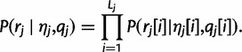
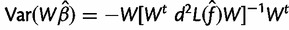
We assume that there are H haplotypes represented in the pool and that the sequence reads have been generated randomly according to the frequencies of the haplotypes. Informally, we use haplotype information contained in an individual read to probabilistically assign that read to one or more of the known haplotypes (fig. 1) and then use the probabilistic haplotype assignments to estimate the haplotype frequencies.

Fig. 1.

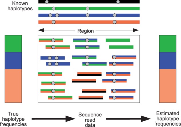
Haplotype information from individual reads can be combined across a genomic region to obtain haplotype frequency estimates. In this cartoon, there are four known haplotypes (black, green, blue, and orange), with sequence data coming from a pool containing 25% green, 25% blue, and 50% orange haplotypes. Each read is probabilistically assigned to the known haplotypes. Some reads can be assigned with great certainty, for example, the reads coming from the blue haplotype that cover two neighboring variant sites. Other reads (represented by two colors) are assigned with less certainty.

Probability Model

Let be the frequencies of the H haplotypes in the genomic region of interest. We can think of N sequence reads as being independently generated as follows. To generate read r_j:

• Choose the haplotype to copy from: .

• Choose a starting position uniformly at random in the genomic region and copy read r_j from haplotype starting at the chosen position.

• Draw base quality scores for the read from a fixed distribution (which can be determined empirically).

• Introduce errors in the sequence read, with the probability of error in a base call given by the base quality score at that position.

In practice, haplotypes may not be perfectly known, or there may be segregating variation within the strain represented by a particular haplotype. In such cases, International Union of Pure and Applied Chemistry ambiguous base codes (e.g., R for purine, Y for pyrimidine, and N for any) may be used in place of the standard bases (A, C, G, and T) to indicate the uncertainty. We incorporate these cases into our probability model by assuming the true base at each segregating site is sampled from a discrete distribution with probabilities determined by the allele frequencies at that site within the strain (which may be known a priori or assumed to be uniform).

Haplotype Likelihood

Calculating the likelihood of a set of haplotype frequencies given, read data under this model can be carried out as follows. Let L_j be the length of the read r_j, let be the base calls, and let be the base quality scores. Also, let be the corresponding bases of haplotype . At read position i, is the probability of sequencing error at that position: . Note that for paired-end data, r_j represents a read pair coming from a single haplotype and that the positions within the read may not be contiguous.

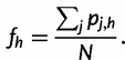
We have . The first term is given by the discrete distribution with probabilities f, and the second term , the “haplotype likelihood,” can be calculated from the base quality scores, as follows.

First, we assume that sequencing errors within a single read are independent of each other:

Next, we need to specify how to calculate the terms in the above product, that is, the probability of an observed base, given the true base and the base quality at that position. For simplicity, we assume that each of the three incorrect bases will be observed with equal probability:

More generally, we note that we can use a base error matrix (parametrized by base quality score) to allow for unequal probabilities and that these probabilities can be estimated from the data by considering the monomorphic sites in the sample.

Note that if position i is a segregating site in the strain represented by haplotype , the likelihood is calculated by summing over the possible bases:

where is the frequency of base b at that site within the strain. For sites where the possible bases are known, but not the allele frequencies, we set the allele frequencies to be equal, for example, 0.5 for biallelic sites and 0.25 for sites with no information.

For clarity, we suppress the dependence on the base quality scores in what follows.

Simple Approaches

We explored two simple approaches for estimating haplotype frequencies. The first method is a simple string match algorithm, where sequence reads are fractionally assigned (with equal weight) to haplotypes with which they are identical up to a specified maximum number of mismatches. For example, a read that matches two haplotypes is assigned 0.5 to each. The fractional assignments are then summed, to obtain counts for each haplotype, and dividing by the number of reads gives the haplotype frequency estimate.

The second method, which we call a “soft” string match, uses the probability model described earlier to calculate the vector of haplotype likelihoods l_j for each read r_j. Thus, the soft string match makes use of the base quality scores from the reads. The haplotype likelihood vector l_j is normalized, so that the components sum to 1, which we take to be our probabilistic haplotype assignment. As with the fractional assignments above, the probabilistic assignments are averaged to obtain the haplotype frequency estimate.

EM Algorithm

In addition to the simple approaches, we developed a full likelihood approach to obtain maximum likelihood estimates of the haplotype frequencies under the probability model described earlier.

We assume that our reads are generated independently, so our complete data likelihood is:

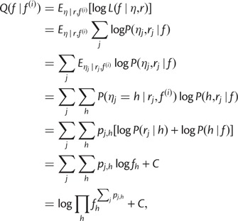
We observe the reads r but treat the haplotype assignments η as missing data, so we are interested in the marginal likelihood,

which we maximize by iteratively calculating haplotype frequency estimates by the EM algorithm:

First we describe the iteration step of the algorithm; we assume we have and show how to obtain . In section Materials and Methods, we show that this is the formal EM algorithm of Dempster et al. (1977).

We let and let be the vector of haplotype likelihoods for read j. Note that for a given sequence read r_j, the haplotype likelihood vector l_j is determined by the variant sites covered by the read, up to a proportionality constant. Also note that the haplotype likelihood vectors can be calculated once and cached, before the actual EM iteration.

Given , we define to be the haplotype posterior vector for read j, where

Intuitively, p_j is a probabilistic haplotype assignment of read r_j, with each component representing the probability that the read came from haplotype h (given our current haplotype frequency estimate ). Note that:

so p_j can be obtained by taking the component-wise product , and normalizing, so that the vector components sum to 1. As a special case, if is uniform, then in the first iteration, p_j is just l_j normalized.

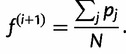
Our updated estimate is given by the average of the haplotype posterior vectors:

Finally, we must specify how to choose our initial haplotype frequency estimate , as well as convergence criteria for the iteration. For our first initial estimate, we use the uniform distribution . We also use additional random initial estimates drawn from a symmetric Dirichlet distribution to start multiple runs of the algorithm, because there is a possibility that the EM algorithm will climb to a nonglobal local maximum on the likelihood surface. For the termination condition, we specify a threshold ε and halt the iteration when the squared distance between estimates falls below the threshold: . In practice, we found a value of to work well, and this value is used in the results presented below.

Base Quality Score Recalibration

We observed inconsistencies between the reported base quality scores in our experimental data sets and empirical error rates based on sequence reads covering monomorphic sites in the known haplotypes (see Results), which motivated the development of a recalibration method to correct for these inconsistencies.

Illumina base quality scores have different interpretations, depending on the Illumina version. In our experimental data set, corresponding to Illumina versions 1.5–1.7, the scores range from 2 to 40, with the score q representing an error probability given by the Phred scale:

For example, a base quality score of 20 gives an error probability of 1/100. The special score of 2 indicates that the base should not be used in downstream analysis.

To recalibrate, we examine monomorphic sites to calculate an observed error rate for each possible base quality score q. These observed error rates can then be used directly in the haplotype likelihood calculation in place of the Phred scale error rates or to create a new BAM file with recalibrated base quality scores.

Haplotype Likelihood Filtering

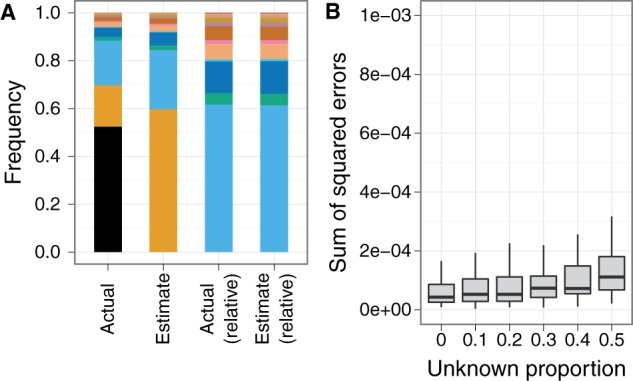
The EM algorithm described earlier relies on the assumption that we know the sequences of the haplotypes found in the pool and that the pool has no contamination from unknown species. Although investigating the effects of unknown haplotypes species in the pool, we found that in the case where the unknown is sufficiently unrelated to the known haplotypes (known species, in the case of 16S sequences), reads from the unknown can be filtered out on the basis of the haplotype likelihoods.

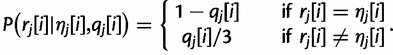
For each sequence read, the maximum haplotype likelihood will usually be attained by the haplotype from which the read was derived. Building on this, we can calculate the distribution of the maximum haplotype likelihood of the sequence reads under the assumption that the pool contains only known haplotypes, based on the empirical base quality score distribution of the data (see Materials and Methods for details). Using this “null” distribution, we can filter out reads whose maximum haplotype likelihood falls outside a specified range (fig. 8A). In our simulations, we obtained good results by filtering out reads whose maximum haplotype likelihood was less than 2 standard deviations (SDs) below the mean of this distribution (fig. 8C).

Fig. 8.

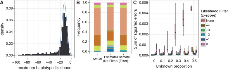
Sequence reads from unknown unrelated species push frequency estimates toward the uniform distribution; filtering the reads based on haplotype likelihood minimizes this effect. (A) Sequence reads from unknown unrelated species have low maximum haplotype likelihoods, giving rise to the long left tail of the distribution. By calculating the theoretical distribution (blue) of maximum haplotype likelihoods based on the base quality scores from the sequence data, reads whose maximum haplotype likelihood falls below a specified threshold (red, z-score threshold = −2 in this example) can be filtered out. (B) A typical example of this effect, with 50% of the reads coming from the unknown species. (C) Without filtering on the haplotype likelihoods, error in frequency estimates increases with higher proportion of unknown sequence reads. Seventy-five-base-pair single-end 16S sequence reads were simulated from 20 species, with varying proportions of reads from an unknown unrelated species (100× pooled coverage, 100 replicates per unknown proportion level).

Results

Comparison with Existing Allele-Frequency-Based and Simple Sequence-Based Methods

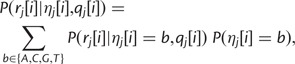
We first evaluated the performance of the EM algorithm in comparison to single-site allele-frequency-based methods and the simple-sequence-based methods discussed earlier (see New Approaches). To represent the allele-frequency-based methods, we chose hippo, which is a freely available program that has been shown to outperform other allele-frequency-based methods for estimating haplotype frequencies (Pirinen 2009). One property of this class of methods is that all possible haplotypes in the region are considered during the estimation. This results in an exponential growth in the number of haplotypes (and thus memory usage and algorithm running time) as the region width increases. To improve performance, the hippo method allows one to specify known haplotypes, which we do here. We found it difficult to obtain results on our simulated data for regions larger than approximately 2 kb (though this distance scale is driven largely by the relatively high Drosophila-specific levels of diversity we simulated here).

In this comparison, we simulated data from a pool of 20 haplotypes with 100-bp paired-end sequence reads and 200× pooled coverage, with 100 replicates each from genomic regions ranging in size from 500 bp to 50 kb.

We found that the simple methods using sequence reads (string match and soft string match) outperformed the method based on single-site allele frequencies and that the EM algorithm performed vastly better than all the other methods (fig. 2). The soft stringmatch method showed a distinct improvement over the stringmatch method, due to the incorporation of information from the base quality scores. We also note that the EM algorithm performed the estimation using 162 reference haplotypes and accurately reported zero frequencies for the haplotypes not present in the pool.

Fig. 2.

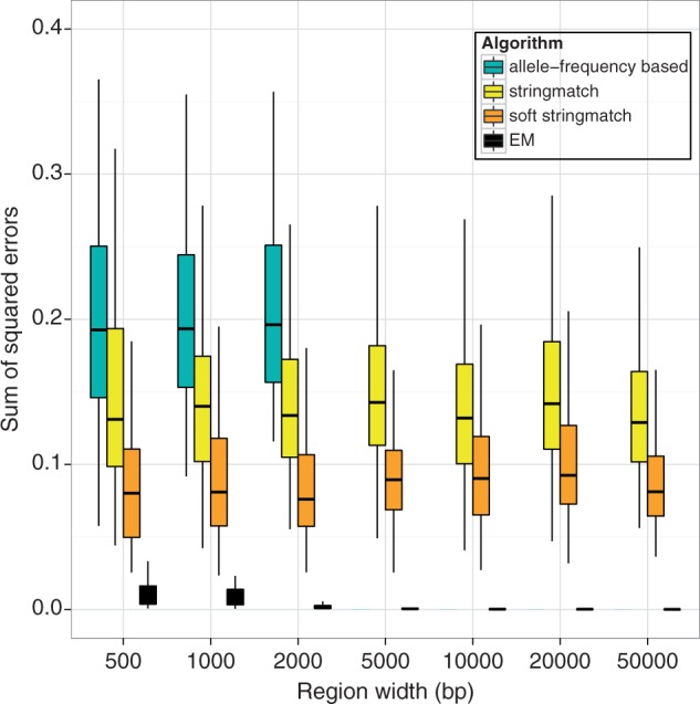
Comparison of the EM algorithm to known allele-frequency-based and simple-sequence-based methods. Each algorithm was run on simulated pooled 100-bp paired-end sequence data from 20 haplotypes at 200× coverage, with 100 replicates for each region width.

The EM algorithm’s increased performance can be attributed to the sharing of information across all the reads in the genomic region. In contrast to the other methods, the EM algorithm’s performance improves as the width of the region increases. This improvement comes from the fact that more variant sites are available to distinguish between haplotypes, in addition to the increased amount of data on which to base the inference.

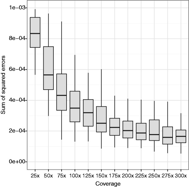
Effects of Region Width, Coverage, Read Length, and Sequencing Error

We next evaluated the performance of the EM algorithm with respect to increasing region width and coverage. In this evaluation, we simulated pooled data (100-bp paired end) from all 162 haplotypes, 100 replicates each in genomic regions ranging in size from 25 to 400 kb, at coverages ranging from 25× to 300×. We found that performance increases substantially as coverage increases, especially at the lower coverage levels (25×–100×) and also as the region width increases (fig. 3A). In particular, for larger regions (100 kb) at moderate pooled coverage (200×), the sum of squared errors is less than , which corresponds to a root mean squared error of less than 0.1% per haplotype.

Fig. 3.

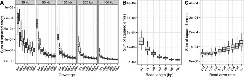
Performance of the EM algorithm increases with coverage, region width, and read length and is robust to sequencing errors. (A) Performance of the EM algorithm increases with both coverage and width of the region used for the estimation. (B) The EM algorithm performs better with longer reads, which provide more haplotype information. (C) The EM algorithm maintains good performance with increasing sequence read error rate. Empirical error rates were found to be in the range of 0.05–0.07 errors per base call. In all simulations, we simulated paired-end pooled sequence data from 162 haplotypes at randomly drawn frequencies, with 100 replicates per parameter value level. Nonvarying parameters were held at fixed values representative of our experimental data (read length 100 bp, read error rate 0.06, coverage 200×, and region width 200 kb).

We also evaluated the effect of increasing read lengths on the performance of the EM algorithm. We simulated paired-end sequence data in a 200 kb region with sequence read lengths ranging from 50 to 500 bp (100 replicates each). In each case, we generated 200,000 read pairs (200× coverage for 100-bp reads). As expected, longer read length also increases performance, due to the additional haplotype information contained in individual reads (fig. 3B). Note that the effect of increased read length is equivalent to the effect of increasing SNP density, due to the fact that differences in haplotype likelihoods between strains/species are determined by the variant sites covered by the sequence reads.

Finally, we studied the effects of sequence read errors on the haplotype frequency estimation. We calculated an empirical base quality score distribution, which we shifted to obtain simulated data sets with specified error rates. In our experimental data sets, the sequence error rate calculated from the base quality scores was generally in the range of (errors per base call), depending on the region. On simulated data sets (162 haplotypes, 200 kb region, 100-bp paired-end reads, 200× coverage), we found that the EM algorithm maintains good performance (sum of squared errors , average error < 0.1%), even with error rates of 2–3× empirical error rates (fig. 3C).

Effects of Haplotype Diversity

We investigated the effects of haplotype diversity, quantified by the Shannon entropy (in natural log units) of the true haplotype frequency distribution, on the performance of the EM algorithm. We simulated pooled 100-bp paired-end sequence data from 162 haplotypes at 200× coverage in a 200-kb region. We generated the haplotype frequencies using symmetric Dirichlet distributions with parameter values ranging from 0.005 to 10, for a total of 550 replicates, which were binned by Shannon entropy (fig. 4). We found that the EM algorithm performs best for low entropy frequency distributions, where there are a few haplotypes at high frequencies, with the rest at low frequencies. Performance degrades as the entropy increases, with a slight improvement for high-entropy (nearly uniform) distributions. This behavior can be explained by the fact that missing information leads to uniform estimates, which will give better results for near-uniform distributions.

Fig. 4.

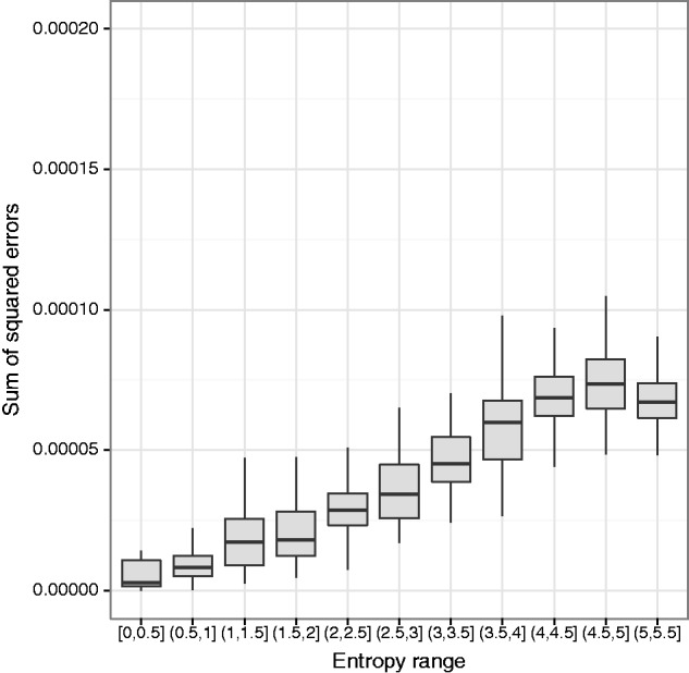
The EM algorithm performs best when the true frequency distribution has low entropy (nonuniform, with a few haplotypes at high frequencies, with the rest at low frequencies). The algorithm was run on simulated pooled 100-bp paired-end sequence data from 162 haplotypes at 200× coverage in a 200 kb region (550 replicates binned by Shannon entropy in natural log units).

Effects of Inaccurate Base Quality Score Reporting

The computation of haplotype likelihoods is dependent on the correct reporting and interpretation of base quality scores. By looking at monomorphic sites in our experimental data sets, we calculated an observed error rate for each possible base quality score, which maps to an empirical base quality score q_obs according to:

We observed that the reported base quality scores in our experimental data sets were consistently inaccurate (fig. 5A). This motivated the development of a recalibration method to correct for inaccurate reporting of base quality scores (see New Approaches).

Fig. 5.

Recalibration of base quality scores using monomorphic sites improves performance. (A) Reported base quality scores do not match empirical scores calculated from real data using monomorphic sites. (B) The EM algorithm was run with and without base quality score recalibration on simulated pooled 100-bp paired-end sequence data from 162 haplotypes at 200× coverage in a 200 kb region (100 replicates each). Sequence errors in the simulated data were introduced with probabilities given by the empirical error rates.

To test our recalibration method, we simulated data sets (162 haplotypes, 100-bp paired-end reads, 200 kb region, 200× coverage) using the empirical error rate for each base quality score to generate sequence read errors. For each of 100 replicates, we ran the EM algorithm with and without recalibration of the base quality scores. We found the algorithm has higher accuracy with the base quality score recalibration (fig. 5B).

Random Initial Estimates to Avoid Local Maxima

We investigated the possibility that the EM algorithm could converge to nonglobal local maxima on the likelihood surface. We simulated data sets (162 haplotypes, 100-bp paired-end reads, 200× coverage, empirical error rates) over a range of region sizes from 10 to 200 kb, starting from a uniform initial estimate in addition to a varying number of random initial estimates (0, 25, 50, and 100), with 100 replicates for each combination. We found that running the algorithm multiple times with random initial estimates did not improve performance (data not shown), indicating that the EM algorithm finds the global maximum reliably starting from a uniform initial estimate.

Estimation of Relative Abundances of Species Based on 16S rRNA Sequence Reads

Although our primary motivation for developing this method arises in the context of Drosophila evolution experiments, the structure of our algorithm suggests it may be extended to the problem of inferring bacterial community composition. For instance, sequence reads derived from 16S rRNA are often used to identify the species contained within a naturally pooled sample. In the context of our method for haplotype frequency estimation, each species with a canonical 16S sequence is a known haplotype, and the challenge is to infer the haplotype frequencies based on reads copied with error from the canonical sequences. As such, our method differs from most existing 16S analysis pipelines in that we do not first classify reads to species and then infer frequencies. As in the haplotype frequency inference problem, we consider the probability of each read coming from each potential source species and then iteratively converge on a set of frequency estimates using the EM algorithm.

As a preliminary test of this approach, we simulated simple communities composed of pools of 200 randomly chosen species (average 16S sequence divergence 19% [±2 SD of 12%]), with 75-bp single-end sequence reads derived from their 16S sequences, at varying coverage levels. The simulated data reflect what one would expect from a shotgun sequencing metagenomics experiment, with sequence reads coming from random locations in the 16S sequence, from the different species according to their relative abundance within the pool. (We do not consider the accuracy for approaches that target a specific hypervariable region, though the algorithm can be applied to such designs.) Figure 6 shows the performance as a function of coverage. As one example, with 150× pooled coverage of the 16S sequence, the average sum of squared errors was , which corresponds to an average error of 0.1%. This error is of the same order of magnitude as the error in estimation of Drosophila strain-level frequencies, which used much larger regions, but typically have lower levels of between-haplotype divergence. In these examples, we assumed the species in the pool are known. We next considered inference settings with unknown species in the pool.

Fig. 6.

Performance of the EM algorithm on the calculation of species-level abundances from 16S rRNA sequence data. The algorithm was run on simulated 75-bp single-end 16S sequence data from pools of 200 randomly chosen microbial species, with 100 replicates for each coverage level.

Frequency Estimation for a Specified Set of Species within a Larger Mixture of Unknown Species

First, because the species of some genera are better characterized than others, we investigated the utility of this method in estimating the frequencies of known species within a single genus, in a pool containing a large number of unknown species from different genera. To this end, we simulated pools containing 500 randomly chosen species: 20 from genus Clostridium, together with 480 species from other genera. In these simulations, the pool of known sequence reads was spiked with unknown sequence reads, with the total unknown proportion ranging from 0% to 50%, and where the unknown sequence reads were drawn uniformly at random from the 480 unknown species. The 16S average sequence divergence between pairs of known species was 12% (%), whereas the average divergence between known and unknown species was 20% (%).

We then estimated the frequencies of the Clostridium species using only the known reference sequences. We found that the EM algorithm, in combination with the haplotype likelihood filter (see New Approaches), performed well (sum of squared errors , average error %), in spite of the large number of unknown species in the pool (fig. 7).

Fig. 7.

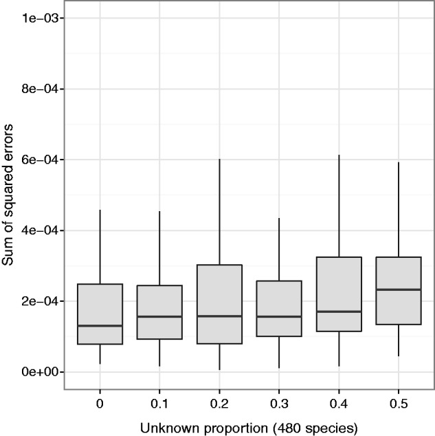
Large numbers of unknown unrelated species do not significantly affect the estimate of within-genus species frequencies. The EM algorithm with haplotype likelihood filter was run on simulated 75-bp single-end 16S sequence reads from 500 species (20 Clostridium species [known] and 480 non-Clostridium species [unknown]). “Unknown proportion” is the total proportion of reads coming uniformly at random from the 480 unknown species, with the remainder of the reads coming from the 20 known species (100× pooled coverage, 100 replicates for each unknown proportion level).

Effects of Unrelated Unknown Species on Frequency Estimation

To more fully characterize the effect of unknown species on the estimation of frequencies of known species, we further investigated the scenario where there are unknown species present within the pool. For simplicity, we simulated pools with 20 known species, spiked with a single unknown species that does not belong to the same genus as any of the known species.

In this situation, reads coming from the unrelated unknown species do not map well to the reference sequences of the known species. Because the unknown is unrelated to the known species, these reads have low haplotype likelihoods across all the known species (fig. 8A). The result is that the frequency estimates are pushed toward a more uniform distribution (fig. 8B), as the reads of the unknown species give weight to all the known species in roughly equal portions. We found that this effect can be minimized by implementing a haplotype likelihood filter (see New Approaches), which effectively keeps only those reads that come from the known species. Our simulations show that a haplotype filter z-score threshold of −2 works well to maintain good performance in the presence of unrelated unknowns (fig. 8C). Without the haplotype filter, performance of the EM algorithm degrades as the proportion of the unknown species in the pool increases.

Effects of Related Unknown Species on Frequency Estimation

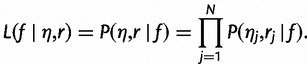
We also investigated the scenario where there is a single unknown species that is related to one of the known species in the pool. Again for simplicity, we simulated pools with 20 known species, spiked with an unknown species from the same genus as one of the known species.

We found that, in general, the sequence reads coming from the unknown species increase the estimated frequency of the known species that it is related to. However, this effect depends on the sequence similarity between the unknown and the related known species. Reads that come from a region where the two species differ significantly are filtered out and do not contribute to the estimation.

This effect is limited to the estimate of the frequency of the known species that is related to the unknown and has little effect on the relative frequency estimates of the other species (fig. 9A and B).

Fig. 9.

When the pool contains an unknown species that is related to one of the known species, sequence reads from the unknown increase the frequency estimate of the most closely related known species but have little effect on the estimation of the relative frequencies of the other known species. (A) Sequence reads from an unknown species (black) related to one of the known species (orange) contribute to the frequency estimate of that species. Shown is a typical example of this effect, with 50% of the reads coming from the unknown species. The relative abundances of the other known species are estimated accurately. (B) Presence of the unknown species has little effect on the estimation of the relative frequencies of the other (unrelated) known species. Seventy-five-base-pair single-end 16S sequence reads were simulated from 20 known species and 1 unknown related species (100× pooled coverage, 100 replicates for each unknown proportion level).

Discussion

We have presented a new method for estimating the frequencies of known haplotypes from pooled sequence data, using the haplotype information contained in individual sequence reads.

We showed that the method outperforms methods based on allele frequencies, as well as simple methods using sequence data. Using data from larger genomic regions improves the accuracy of the estimate. Increased coverage and longer read lengths also improve the performance of the algorithm. The method generally performs better for haplotype frequency distributions with lower entropy (nonuniform) than those with higher entropy (uniform), which is particularly notable in metagenomics contexts, where species/strain abundances are far from uniform. The method incorporates uncertainty in the sequence reads by using the reported base quality scores. Recalibration of base quality scores using monomorphic sites in the pooled data leads to better performance.

We note that in the EM algorithm, as well as the two simple approaches, haplotype information from individual sequence reads is combined across a genomic region, which minimizes the effects of local areas of low coverage. In contrast, single-site allele frequency estimates have larger variance at sites with lower coverage, which decreases the accuracy of methods based on these estimates.

The method relies on the probabilistic assignment of sequence reads to the known haplotypes. The method works best when the SNP density (the number of SNPs per base pair) is high; ideally, individual read pairs will cover multiple SNPs. In the DGRP Drosophila strains, the SNP density is SNP/bp, so that 100-bp paired-end reads contain on average 10 SNPs per pair, which is sufficient for this probabilistic assignment. As sequence read lengths increase with advances in sequencing technology, we anticipate that this method will be useful for a wide variety of organisms.

This method can be improved to handle more complicated genomic situations. For example, the probability model described could be enhanced with known information about between-species or between-strain copy number variation. In addition, because estimation at the species level (or above) requires mapping the reads to multiple references, there is room for improvement in the efficiency of this step, including methods for mapping reads to multiple references simultaneously with automatic calculation of haplotype likelihoods, which can then be input directly into the EM iteration.

This method has immediate application in the analysis of pooled data from artificial selection experiments where the founding haplotypes are known. In essence, by using information from the founding population, we are able to infer haplotype information about the final pooled population, which has previously only been available when individuals have been sequenced separately. This haplotype information can then be used for various purposes (e.g., to look for signatures of selection).

It should be noted that in the experimental evolution setting, the haplotype frequency estimates obtained are local and will vary across the genome due to recombination over the course of the experiment. In the case where a recombination has occurred within the region under consideration, nearly all sequence reads coming from the recombined haplotype will come from one or the other of the two original haplotypes. Because of this, reads from the recombined haplotype will contribute to the frequency estimates of both of the original haplotypes, with the exact proportion determined by the location of the recombination point within the region. The few reads that span a recombination point will have very low haplotype likelihoods and will contribute negligibly to the final estimate. In practice, one can choose the width of the genomic region used for the estimation to be smaller than the expected length scale of recombination. For example, in Drosophila selection experiments lasting 25 generations, we expect to see recombination breakpoints at a scale of , whereas our method obtains very accurate results with much smaller regions of .

Haplotype frequency estimation from pools may also be useful in quantitative trait loci (QTL) mapping studies. In studies with recombinant inbred lines, several generations of inbreeding are carried out with lines that are derived from mixed populations founded by multiple strains, and the parent of origin for each segment in each inbred line is inferred and correlated with phenotypic trait values. As an alternative, it may be possible to perform haplotype frequency estimation from pooled sequencing of the mixed populations directly and map traits by correlating haplotype frequencies with trait values.

In addition to applications in experimental evolution settings with known founder haplotypes, we also explored whether the method may have utility for estimating the relative abundances of known species from metagenomic data. We specifically tested the setting in which one has short-read shotgun sequencing data from 16S rRNA, rather than amplicon-based 16S rRNA sequences. The setting we have tested is relevant to the practical setting in which one generates whole-genome metagenomic data and then focuses on reads from 16S rRNA for quantification of known species. In our simulation experiments, we have explored various factors affecting performance. We note how having closely related species in the sample that are not in the reference set will elicit an implicit “clustering” behavior, in which the most closely related known species in the reference set will have its frequency inflated (fig. 9A). The relative frequencies of unrelated species are not affected, however (fig. 9B). This behavior extends nicely to the case where one is interested in the relative frequencies of species from a well-characterized genus (e.g., one in which most member species have known canonical 16S rRNA sequences). In this case, we show that the relative frequencies can be estimated well, even in the presence of hundreds of background species (fig. 7). In these cases, our haplotype likelihood filter acts as a form of clustering tool in that we only base the frequency estimates on reads that are close to the taxa of interest.

Just as SNP density is highly relevant in the haplotype inference problem, a key factor in the performance for metagenomic applications is the amount of 16S sequence divergence between the taxa of interest. Our examples were based on species sets whose divergences were generally between 5% and 33% and the method performed well in these settings. More closely related species will be more difficult to distinguish, and at an extreme, strains within species will require more than the 16S sequence to distinguish. One limitation is that our method infers frequencies of taxa represented by specific canonical rRNA sequences. How our method would perform with a single canonical sequence per genus, class, or phylum is not clear, and future extensions of this work may seek to specifically alter the underlying probability model to include diversity within taxa to specifically address this problem.

The potential advantage over existing methods for handling 16S data lies in the method’s ability to handle base quality scores explicitly and give probabilistic weights to the source of reads, rather than making hard classifications and estimating frequencies based on those classifications. As we have shown in the context of haplotype frequency estimation (fig. 2), such estimation performs much worse than the probabilistic approach we take here.

The software implementing the method, harp, is open source and available for download and can be easily integrated into existing analysis pipelines.

Materials and Methods

Implementation

We implemented both simple approaches and the EM algorithm described earlier in a C++ program called harp (“Haplotype Analysis of Reads in Pools”). The program takes as input a standard BAM file with mapped sequence reads, a reference sequence in FASTA format, and known haplotypes in the SNP data format used by the DGRP project (Mackay et al. 2012). Alternatively, to estimate abundances of distinct species within a pool, the program will accept multiple BAM files, each paired with the reference sequence used for the read mapping. The software uses the samtools API for random access to BAM files (Li et al. 2009). The program includes many options for the user to customize the analysis, including choice of algorithm, the genomic region to analyze, parameters for sliding windows within the region, convergence threshold for the EM algorithm, parameters used to generate multiple random initial estimates to avoid local maxima, base quality score recalibration, and haplotype likelihood filtering threshold. The program also calculates standard errors for the haplotype frequency estimates, using general properties of the EM algorithm and maximum likelihood estimators (details on this calculation below).

Performance Evaluation

We used the following procedure to simulate pooled sequence data:

• Draw a random haplotype frequency distribution (the “true” distribution) from a symmetric Dirichlet distribution. The symmetric Dirichlet distribution is parameterized with a single parameter α that governs the uniformity of the randomly drawn frequency distributions: gives an identical probability to each possible frequency distribution, generates frequency distributions that are close to uniform (i.e., all haplotypes at similar frequencies), and generates frequency distributions that are more nonuniform (i.e., a few common haplotypes, and many rare ones). The parameter value was chosen to produce frequency distributions with nonuniformity similar to that observed in our experimental Drosophila data.

• Draw random sequence reads by choosing the haplotype according to the true distribution and the starting position uniformly at random over the given genomic region. For paired-end reads, the paired-end distance was chosen according to a Poisson distribution fitting the experimental Drosophila data.

• For segregating sites denoted by ambiguous base codes, draw allele frequencies according to a symmetric Dirichlet distribution. Choose the true base at a segregating site according to the allele frequencies. (For biallelic sites denoted by a 2-base ambiguous code, e.g., R for A or G, we set the Dirichlet parameter , i.e., the allele frequency was chosen uniformly at random. For sites denoted by N (any) in the haplotype, we set , as we expect that most of these sites have an allele that is at or near fixation.)

• Generate base quality scores according to the empirical distribution obtained from the real data (either Drosophila or 16S) and introduce sequencing errors with error rates determined by the base quality scores.

For the simulated Drosophila pooled sequence data, we generated mapped read files (SAM format), which were subsequently converted to binary format (BAM) using samtools (Li et al. 2009). For the simulated 16S rRNA sequence data, we generated raw read files (fastq format), which were then mapped to reference sequences using bwa (Li and Durbin 2010).

For our performance metric, we used the sum of squared errors between the true haplotype frequencies of the simulated data and the frequencies estimated by the EM algorithm: 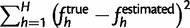, in addition to the root mean squared error. We define f_true to be the realized frequencies of the haplotypes in the sequenced reads from the DNA pool. We do this to quantify the error of estimation, rather than the stochasticity of the pooled sequencing. For the purposes of comparison across simulations, we report the sum of squared errors in the figures. However, we also give the equivalent root mean squared errors in the main text for interpretation.

Simulation of Drosophila Pooled Sequence Data

To evaluate the performance of the algorithms, we used simulated pooled sequence data based on experimental data from selection experiments in Drosophila melanogaster (Turner and Miller 2012). The data consisted of Illumina 85-bp and 100-bp paired-end sequence reads generated from four pools of 120 D. melanogaster individuals each, sequenced at 200× average coverage. For our known haplotypes, we used the publicly available SNP data from 162 Drosophila inbred lines representing Freeze 1 of the DGRP project. The published haplotypes include ambiguous base codes (e.g., R for A or G) to represent sites that have multiple alleles still segregating within the inbred line. The ambiguous base code N is used at sites where there was not enough sequence data to make a base call.

Simulation of 16S rRNA Pooled Sequence Data

To evaluate the ability of the EM algorithm to estimate species abundances from a pool of 16S rRNA sequences, we used sequences from the Greengenes 2011 release of its 16S rRNA sequence database (DeSantis et al. 2006), which consists of approximately 800,000 sequences. We simulated 75-bp single-end sequence reads with an empirical base quality score distribution based on the publicly available Illumina-sequenced “mock community” short read archive data sets from the Human Microbiome Project (NIH HMP Working Group 2009). Specific details on number of species used in each simulated experiment are described in the Results section.

Formal EM Calculation

Expectation Step

We calculate the expectation of the complete data log likelihood, where the expectation is taken over the posterior distribution of the missing data given the observed data and the current estimate. Recall that 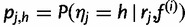is the probability that read r_j came from haplotype h, given our current haplotype frequency estimate .

where C is a constant independent of f.

Maximization Step

Our next estimate is given by the f that maximizes the expected log likelihood:

First note that the function 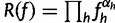is maximized by 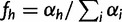. (For example, the maximum likelihood estimator for the parameters of a multinomial distribution is given by the vector of count proportions.)

Because is monotonic and

is maximized when, for all h:

In other words, our next estimate is given by the average of the posterior vectors:

Calculation of Standard Errors

We use general properties of the EM algorithm and maximum likelihood estimators to calculate standard errors for our haplotype frequency estimates, following Lange (2010). For brevity, we let L(f) be the log likelihood of f. Our strategy to calculate standard errors of our maximum likelihood estimate is as follows:

1. Estimate the observed information .

2. is asymptotically normal with covariance matrix , so the standard error estimates are the square roots of the diagonals of .

One slight complication is that our estimate is subject to a linear constraint (the frequencies must sum to 1). Below, we also show how to adjust this calculation to handle this constraint.

Calculating

Let g be the minorizing function for the EM algorithm:

Then g satisfies the relations for all :

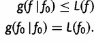Note that 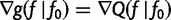. Also, is minimized , so at . This means that . Note that is the gradient computed as a function of f, then evaluated at .

In summary, we can write the score function , defined to be the gradient of the log likelihood, as:

Because , we need to find the partial derivatives of S.

Recall that we have:

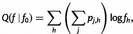where is the haplotype posterior vector, representing the probability that read r_j came from haplotype h.

Note that the depends on f₀, but not f, so the partial derivatives of have a simple form:

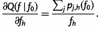Now we evaluate at and drop the subscript:

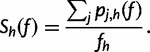We can now compute partial derivatives of the score function:

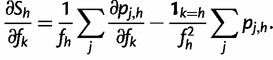To compute the partial derivatives of , first write as:

where 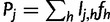is the total probability of read r_j. Because , we have:

Adjusting for the Linear Constraint

We continue to follow Lange (2010) to handle the linear constraint . Let 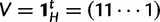be the row vector with H 1’s, so we can write our constraint as .

We let W be a matrix with column vectors orthogonal to V:

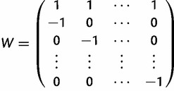We reparametrize by β, using the relation 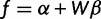, where α satisfies the constraint . As a function of β, the log-likelihood has observed information 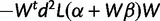, which gives an estimate 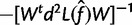. This gives the estimate , where was estimated above.

Haplotype Likelihood Filter Threshold

In this section, we show how we approximate the mean and variance of the maximum haplotype likelihood distribution, which are used to calculate the threshold for the haplotype likelihood filter.

The main idea is that the maximum haplotype likelihood for a read is usually attained by the actual haplotype from which the read was copied. Because of this, we can approximate the mean and variance of the maximum haplotype likelihood distribution by the mean and variance of the distribution of for reads r copied from a fixed haplotype h, under the empirical distribution of the base quality scores q. For ease of calculation and implementation, we actually calculate the statistics for the log-likelihood distribution . We also suppress the dependence on h in the following for ease of notation.

We assume we have an empirical per-position base quality score distribution obtained from the data, where for simplicity we assume that the base quality scores at different positions are independent of each other. So for reads of length L, we have discrete random variables . For example, for Illumina reads, Q_i will take values in . For a base quality score q, we let denote the probability of a read error for that base. Typically we will have the Phred-encoded error probabilities, so .

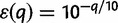Let denote the true haplotype sequence from which the read is copied, denote the base quality scores, and denote the read bases. Note the slight change in notation from the description of the probability model (see New Approaches): Here, the subscript denotes position in the sequence read.

By our assumption of position independence, we have . Note that each of these terms is random:

where the first event corresponds to (no error), and the second event represents the three possible error bases when , each one occurring with probability .

Next we calculate the conditional expectation of given q_i:

Note that this expression does not depend on r_i. Now we can take the expectation over Q_i:

Note that this expression does not depend on either r_i or q_i and is a function solely of the empirical distribution Q_i. Finally, we can sum over positions to obtain:

which represents the expected log haplotype likelihood for a read r corresponding to the true haplotype h, under the empirical base quality distribution.

Similarly, we calculate 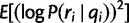for each position, from which we can obtain the per-position variance 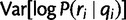. Again by our position-independence assumption, we have:

We use the calculated mean and variance of to translate a user-defined z-score threshold into a haplotype log-likelihood threshold for filtering out low-likelihood reads.

References

- Burke MK, Dunham JP, Shahrestani P, Thornton KR, Rose MR, Long AD. Genome-wide analysis of a long-term evolution experiment with Drosophila. Nature. 2010;467:587–590. doi: 10.1038/nature09352. [DOI] [PubMed] [Google Scholar]
- Cheesman SJ, de Roode JC, Read AF, Carter R. Real-time quantitative PCR for analysis of genetically mixed infections of malaria parasites: technique validation and applications. Mol Biochem Parasitol. 2003;131:83–91. doi: 10.1016/s0166-6851(03)00195-6. [DOI] [PubMed] [Google Scholar]
- Cutler DJ, Jensen JD. To pool, or not to pool? Genetics. 2010;186:41–43. doi: 10.1534/genetics.110.121012. [DOI] [PMC free article] [PubMed] [Google Scholar]
- Dempster A, Laird N, Rubin D. Maximum likelihood from incomplete data via the EM algorithm. J R Stat Soc Ser B. 1977;39:1–38. [Google Scholar]
- DeSantis TZ, Hugenholtz P, Larsen N, Rojas M, Brodie EL, Keller K, Huber T, Dalevi D, Hu P, Andersen GL. Greengenes, a chimera-checked 16S rRNA gene database and workbench compatible with ARB. Appl Environ Microbiol. 2006;72:5069–5072. doi: 10.1128/AEM.03006-05. [DOI] [PMC free article] [PubMed] [Google Scholar]
- Earley EJ, Jones CD. Next-generation mapping of complex traits with phenotype-based selection and introgression. Genetics. 2011;189:1203–1209. doi: 10.1534/genetics.111.129445. [DOI] [PMC free article] [PubMed] [Google Scholar]
- Futschik A, Schlötterer C. The next generation of molecular markers from massively parallel sequencing of pooled DNA samples. Genetics. 2010;186:207–218. doi: 10.1534/genetics.110.114397. [DOI] [PMC free article] [PubMed] [Google Scholar]
- Gasbarra D, Kulathinal S, Pirinen M, Sillanpää MJ. Estimating haplotype frequencies by combining data from large DNA pools with database information. IEEE/ACM Trans Comput Biol Bioinform. 2009;8:36–44. doi: 10.1109/TCBB.2009.71. [DOI] [PubMed] [Google Scholar]
- Hastings IM, Nsanzabana C, Smith TA. A comparison of methods to detect and quantify the markers of antimalarial drug resistance. Am J Trop Med Hyg. 2010;83:489–495. doi: 10.4269/ajtmh.2010.10-0072. [DOI] [PMC free article] [PubMed] [Google Scholar]
- Hastings IM, Smith TA. MalHaploFreq: a computer programme for estimating malaria haplotype frequencies from blood samples. Malar J. 2008;7:130. doi: 10.1186/1475-2875-7-130. [DOI] [PMC free article] [PubMed] [Google Scholar]
- Huang W, Richards S, Carbone MA, et al. (25 co-authors) Epistasis dominates the genetic architecture of Drosophila quantitative traits. Proc Natl Acad Sci U S A. 2012;109:15553–15559. doi: 10.1073/pnas.1213423109. [DOI] [PMC free article] [PubMed] [Google Scholar]
- Human Microbiome Project Consortium. Structure, function and diversity of the healthy human microbiome. Nature. 2012;486:207–214. doi: 10.1038/nature11234. [DOI] [PMC free article] [PubMed] [Google Scholar]
- Hunt P, Fawcett R, Carter R, Walliker D. Estimating SNP proportions in populations of malaria parasites by sequencing: validation and applications. Mol Biochem Parasitol. 2005;143:173–182. doi: 10.1016/j.molbiopara.2005.05.014. [DOI] [PubMed] [Google Scholar]
- Ito T, Chiku S, Inoue E, Tomita M, Morisaki T, Morisaki H, Kamatani N. Estimation of haplotype frequencies, linkage-disequilibrium measures, and combination of haplotype copies in each pool by use of pooled DNA data. Am J Hum Genet. 2003;72:384–398. doi: 10.1086/346116. [DOI] [PMC free article] [PubMed] [Google Scholar]
- Kirkpatrick B, Armendariz CS, Karp RM, Halperin E. HAPLOPOOL: improving haplotype frequency estimation through DNA pools and phylogenetic modeling. Bioinformatics. 2007;23:3048–3055. doi: 10.1093/bioinformatics/btm435. [DOI] [PubMed] [Google Scholar]
- Kofler R, Orozco-terWengel P, De Maio N, Pandey RV, Nolte V, Futschik A, Kosiol C, Schlötterer C. PoPoolation: a toolbox for population genetic analysis of next generation sequencing data from pooled individuals. PLoS One. 2011;6:e15925. doi: 10.1371/journal.pone.0015925. [DOI] [PMC free article] [PubMed] [Google Scholar]
- Kuk AYC, Zhang H, Yang Y. Computationally feasible estimation of haplotype frequencies from pooled DNA with and without Hardy-Weinberg equilibrium. Bioinformatics. 2009;25:379–386. doi: 10.1093/bioinformatics/btn623. [DOI] [PubMed] [Google Scholar]
- Lange K. Numerical analysis for statisticians (statistics and computing) 2nd ed. New York: Springer; 2010. [Google Scholar]
- Ley R, Turnbaugh PJ, Klein S, Gordon JI. Human gut microbes associated with obesity. Nature. 2006;444:1022–1023. doi: 10.1038/4441022a. [DOI] [PubMed] [Google Scholar]
- Li H, Durbin R. Fast and accurate long-read alignment with Burrows-Wheeler transform. Bioinformatics. 2010;26:589–595. doi: 10.1093/bioinformatics/btp698. [DOI] [PMC free article] [PubMed] [Google Scholar]
- Li H, Handsaker B, Wysoker A, Fennell T, Ruan J, Homer N, Marth G, Abecasis G, Durbin R. The Sequence Alignment/Map format and SAMtools. Bioinformatics. 2009;25:2078–2079. doi: 10.1093/bioinformatics/btp352. [DOI] [PMC free article] [PubMed] [Google Scholar]
- Li X, Foulkes AS, Yucel RM, Rich SM. An expectation maximization approach to estimate malaria haplotype frequencies in multiply infected children. Stat Appl Genet Mol Biol. 2007;6:Article 33. doi: 10.2202/1544-6115.1321. [DOI] [PubMed] [Google Scholar]
- Long Q, Jeffares DC, Zhang Q, Ye K, Nizhynska V, Ning Z, Tyler-Smith C, Nordborg M. PoolHap: inferring haplotype frequencies from pooled samples by next generation sequencing. PLoS One. 2011;6:e15292. doi: 10.1371/journal.pone.0015292. [DOI] [PMC free article] [PubMed] [Google Scholar]
- Mackay TFC, Richards S, Stone EA, et al. (52 co-authors) The Drosophila melanogaster Genetic Reference Panel. Nature. 2012;482:173–178. doi: 10.1038/nature10811. [DOI] [PMC free article] [PubMed] [Google Scholar]
- Mizrahi-Man O, Davenport ER, Gilad Y. Taxonomic classification of bacterial 16S rRNA genes using short sequencing reads: evaluation of effective study designs. PLoS One. 2013;8:e53608. doi: 10.1371/journal.pone.0053608. [DOI] [PMC free article] [PubMed] [Google Scholar]
- NIH HMP Working Group. The NIH Human Microbiome Project. Genome Res. 2009;19:2317–2323. doi: 10.1101/gr.096651.109. [DOI] [PMC free article] [PubMed] [Google Scholar]
- Niu T. Algorithms for inferring haplotypes. Genet Epidemiol. 2004;27:334–347. doi: 10.1002/gepi.20024. [DOI] [PubMed] [Google Scholar]
- Nuzhdin SV, Harshman LG, Zhou M, Harmon K. Genome-enabled hitchhiking mapping identifies QTLs for stress resistance in natural Drosophila. Heredity. 2007;99:313–321. doi: 10.1038/sj.hdy.6801003. [DOI] [PubMed] [Google Scholar]
- Orozco-terWengel P, Kapun M, Nolte V, Kofler R, Flatt T, Schlötterer C. Adaptation of Drosophila to a novel laboratory environment reveals temporally heterogeneous trajectories of selected alleles. Mol Ecol. 2012;21:4931–4941. doi: 10.1111/j.1365-294X.2012.05673.x. [DOI] [PMC free article] [PubMed] [Google Scholar]
- Pe’er I, Beckmann JS. Resolution of haplotypes and haplotype frequencies from SNP genotypes of pooled samples. Proceedings of the Seventh Annual International Conference on Computational Molecular Biology—RECOMB ’03; Berlin, Germany. New York: ACM; 2003. pp. 237–246. [Google Scholar]
- Pirinen M. Estimating population haplotype frequencies from pooled SNP data using incomplete database information. Bioinformatics. 2009;25:3296–3302. doi: 10.1093/bioinformatics/btp584. [DOI] [PubMed] [Google Scholar]
- Sabeti PC, Varilly P, Fry B, et al. (248 co-authors) Genome-wide detection and characterization of positive selection in human populations. Nature. 2007;449:913–918. doi: 10.1038/nature06250. [DOI] [PMC free article] [PubMed] [Google Scholar]
- Takala SL, Smith DL, Stine OC, Coulibaly D, Thera MA, Doumbo OK, Plowe CV. A high-throughput method for quantifying alleles and haplotypes of the malaria vaccine candidate Plasmodium falciparum merozoite surface protein-1 19 kDa. Malar J. 2006;5:31. doi: 10.1186/1475-2875-5-31. [DOI] [PMC free article] [PubMed] [Google Scholar]
- Turner TL, Miller PM. Investigating natural variation in Drosophila courtship song by the evolve and resequence approach. Genetics. 2012;191:633–642. doi: 10.1534/genetics.112.139337. [DOI] [PMC free article] [PubMed] [Google Scholar]
- Turner TL, Stewart AD, Fields AT, Rice WR, Tarone AM. Population-based resequencing of experimentally evolved populations reveals the genetic basis of body size variation in Drosophila melanogaster. PLoS Genet. 2011;7:e1001336. doi: 10.1371/journal.pgen.1001336. [DOI] [PMC free article] [PubMed] [Google Scholar]
- Voight BF, Kudaravalli S, Wen X, Pritchard JK. A map of recent positive selection in the human genome. PLoS Biol. 2006;4:e72. doi: 10.1371/journal.pbio.0040072. [DOI] [PMC free article] [PubMed] [Google Scholar]
- Wang S, Kidd KK, Zhao H. On the use of DNA pooling to estimate haplotype frequencies. Genet Epidemiol. 2003;24:74–82. doi: 10.1002/gepi.10195. [DOI] [PubMed] [Google Scholar]
- Yang Y, Zhang J, Hoh J, Matsuda F, Xu P, Lathrop M, Ott J. Efficiency of single-nucleotide polymorphism haplotype estimation from pooled DNA. Proc Natl Acad Sci U S A. 2003;100:7225–7230. doi: 10.1073/pnas.1237858100. [DOI] [PMC free article] [PubMed] [Google Scholar]
- Zhang H, Yang HC, Yang Y. PoooL: an efficient method for estimating haplotype frequencies from large DNA pools. Bioinformatics. 2008;24:1942–1948. doi: 10.1093/bioinformatics/btn324. [DOI] [PubMed] [Google Scholar]
- Zhou D, Udpa N, Gersten M, et al. (11 co-authors) Experimental selection of hypoxia-tolerant Drosophila melanogaster. Proc Natl Acad Sci U S A. 2011;108:2349–2354. doi: 10.1073/pnas.1010643108. [DOI] [PMC free article] [PubMed] [Google Scholar]