Dynamics of DNA Replication in Yeast

Abstract

We present a mathematical model for the spatial dynamics of DNA replication. Using this model we determine the probability distribution for the time at which each chromosomal position is replicated. From this we show, contrary to previous reports, that mean replication time curves cannot be used to directly determine origin parameters. We demonstrate that the stochastic nature of replication dynamics leaves a clear signature in experimentally measured population average data, and we show that the width of the activation time probability distribution can be inferred from this data. Our results compare favorably with experimental measurements in Saccharomyces cerevisae.

DNA replication starts at specific locations in the chromosome called replication origins. Most bacterial genomes are replicated from a single origin, but the much greater size of eukaryotic genomes requires multiple origins per chromosome to ensure that the replication process does not take too long. Genome replication has been comprehensively studied in the model organism S. cerevisiae (brewers’ yeast). Origin locations in S. cerevisiae are determined by specific DNA sequences and are thus fixed in every yeast cell [1]. The positions of origins in yeast have been comprehensively catalogued [2]. However, a given origin may not be active during replication, because origins must be licensed before the start of S phase (the part of the cell cycle where DNA replication takes place). Licensing consists of a series of specific protein complexes binding at origin locations, culminating in the loading of pairs of Mcm2-7 molecules. If in a given cell licensing of a certain origin is not completed by the time S phase starts, the origin is unable to function [3].

High-throughput methods have allowed the measurement of replication times as a function of chromosomal position for the whole genome [4]. These experiments yield average replication times over large cell populations (typically >10⁷ cells) and therefore can mask the cell-to-cell variability present in the system [5]; to date single cell and single molecule studies are not able to measure the kinetics of whole genome replication [5,6]. The low abundance of the molecules involved in triggering origin activation strongly suggests that origins have stochastic activation times [7]. This is often ignored in the biological literature, where there is a pervasive notion of a “replication program,” in which origins are considered to be programmed to fire following a precisely controlled order. This idea has frequently led to erroneous interpretations of replication time profiles (reviewed in [8]).

There has been much interest recently in mathematical modeling of DNA replication. Two different modeling approaches have been used: simulations to capture the replication dynamics at a single cell level [9-12], and probabilistic models that characterize the dynamics of replication at a population level [13,14]. Some models of DNA replication [14,15] are closely related to Kolmogorov’s classical model of nucleation processes [16]. Our model can be regarded as an inhomogeneous model of nucleation with quenched disorder, where nucleation starts at specific sites. Inhomogeneous models of nucleation have been studied in the context of statistical physics and have relevance to surface science and other areas [17,18].

Reference [14] is particularly relevant for this work because it proposes that origins fire stochastically in time, and goes on to show that this can lead to reproducible replication dynamics population wide, without the need to invoke a “replication program.” Although valuable insights have been gained from previous works, they ignore the possibility that origins can fail to license, and we will show that this has a crucial effect on the system’s dynamics. In addition, most of the existing models are numerical. In this work, we introduce an analytical model of eukaryotic DNA replication which fully takes into account the stochastic nature of both origin activation and the licensing process. Using a simple two-origin chromosome, we illustrate how replication time curves from measurements are influenced by the stochasticity of origin activation as well as by the possibility that licensing fails, reinforcing results we obtained previously by direct simulations [8]. We establish that the shape of the average replication time profile has a signature of the stochasticity of the replication process, even though it is a quantity defined by a population average. We derive an analytical expression relating the replication time in the regions between two origins to the standard deviation Δt of the activation time distribution of the origins. This is a valuable result, since few single cell experiments have been able to give direct information about the stochastic properties of the replication dynamics. Our results allow Δt to be obtained from widely available population-wide measurements. We apply this result to measured replication time data, and estimate Δt from the data, obtaining a result in agreement with current estimates in the literature.

In our model we consider a chromosome with N origins, where each origin i is defined by the following: its chromosomal position x_i; the probability q_i that the origin achieves licensing (in a given cell within a population) and is thus capable of activating; and the activation time probability distribution p_i(t), which is the probability density of origin i activating and starting bidirectional replication forks at time t. Since an origin may not be competent in every cell within the population, in general q_i < 1, and p_i satisfies ${\int }_{-\infty }^{+\infty }{p}_i\left(t\right)dt=q_i$. The fundamental quantity from which all statistical properties of this system can be calculated is the probability density P(x, t), defined such that P(x, t)dt is the probability that chromosomal position x is replicated between times t and t + dt. If only origin i were present, P would be given by P(x, t) = p_i(t − |x − x_i|/v), where v is the fork velocity, which we assume to be a constant.

In the presence of all N origins, the calculation of P(x, t) is complicated by the fact that position x can be replicated by forks originated from any of the origins. Let us assume that position x is replicated between times t and t + dt by a fork from origin i. This requires that (i) origin i activated at time t − |x − x_i|/v, so that the fork arrives at x at time t; and (ii) all other origins j ≠ i have either not activated or they have activated but their forks would arrive at x later than t. The probability density for event (i) is p_i(x, t) = p_i(t − |x − x_i|/v, and the probability for event (ii) is $Q_i(x,t)={\Pi }_{j\ne i}{M}_j(x,t)$, where M_i is the probability that a fork from origin i arrives later than t, or fails to activate: $M_i(x,t)=s_i+{\int }_t^{+\infty }{p}_i(x,y)dy$, where s_i = 1 − q_i is the probability of origin i not being competent. Therefore, the probability density P_i(x, t) that position x is replicated by origin i at time t is

$$P_i(x,t)=p_i(x,t)Q_i(x,t).$$ (1)

Finally, the probability density that position x is replicated at time t, irrespective of which origin the fork started from, is

$$P(x,t)=\sum _{i=1}^N{P}_i(x,t).$$ (2)

One of the most important quantities for comparison with experimental data is the average replication time T(x) at position x, which is given in terms of P as

$$T\left(x\right)=\frac{1}{1-s_1{s}_2\cdots s_N}{\int }_{-\infty }^{+\infty }tP(x,t)dt,$$ (3)

where $1-s_1{s}_2\cdots s_N={\int }_{-\infty }^{+\infty }P(x,t)dt$ is the probability that at least one of the origins will activate. The average replication time across whole chromosomes [T(x) curves] has been measured in a number of organisms. However, caution is required when interpreting T(x) curves. In some of the biological literature, T(x) curves are used to directly infer origin parameters [4]. For example, it is widely accepted that the values of T at x_i are the average activation times of origins. However, Eq. (3) shows that T(x) is determined collectively by all origins [8]. This suggests that simple interpretations of T(x) are not justifiable.

We want to use the general theory presented above to study replication dynamics in a simple setting. From now on we focus on the case of a hypothetical linear chromosome with just two origins. We define the chromosomal coordinates so that one of the origins has position x₁ = 0; the other origin has position x₂ = D. We assume for simplicity that each origin can activate within a time window Δt with uniform probability; we will argue later that our conclusions are largely independent of the precise shape of the probability distribution. We select origin activation times so that the average activation time of the first origin is 0. The other origin has an average activation time τ, and we assume without loss of generality that τ ≥ 0. Thus the activation time distributions are

$$p_i\left(t\right)=\frac{q_i}{\Delta t},ift\in \left[t_i^{\mathrm{av}}-\frac{\Delta t}{2},t_i^{\mathrm{av}}+\frac{\Delta t}{2}\right],$$ (4)

where i = 1, 2, $t_1^{av}=0$, and $t_2^{av}=\tau$. p₁ and p₂ are set to zero outside the stated intervals.

Using Eqs. (3) and (4), we can write analytical expressions for the probability density P(x, t) and the average replication time T(x). From Eq. (4) and (2), P(x, t) vanishes outside the intervals I₁ and I₂ given by

$$I_i=\left[\frac{\mid x_i-x\mid }{v}+t_i^{\mathrm{av}}-\frac{\Delta t}{2};\frac{\mid x_i-x\mid }{v}+t_i^{av}+\frac{\Delta t}{2}\right],$$ (5)

where x₁ = 0 and x₂ = D. In total there are five scenarios (depending on the relative values of τ, Δt, D, and v) that differ in the dynamics of how the chromosome is replicated. From here on we will consider just the case where the condition τ + Δt < D/v is satisfied, since this is the case for many pairs of origins in real chromosomes. This means that the variations in the activation time Δt are small enough that a fork from one origin can only replicate the other origin if that origin is not competent. The expression for T(x) is then

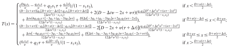(6)

A plot of T(x) for different values of q₁ is shown in Fig. 1. We see that T(x) has discontinuous derivatives at the origin locations, because the forks originate there. At the origins, the mean replication times are

$$\begin{array}{cc}\hfill T\left(x_1\right)& =T\left(0\right)=q_2{s}_1(D∕v+\tau )∕(1-s_1{s}_2);\hfill \\ \hfill T\left(x_2\right)& =T\left(D\right)=(q_1{s}_{2}D∕v+q_2\tau )∕(1-s_1{s}_2).\hfill \end{array}$$ (7)

It is commonly assumed in the replication literature that T(x) has a minimum at an origin, and that the value of this minimum directly gives the average activation time for the origin. However, Eq. (7) shows that this is not the case and, in fact, $T\left(x_i\right)\ge t_i^{av}$: the mean replication time at an origin location is equal to or greater than the origin’s average activation time. Only when an origin has q_i = 1 can $T\left(x_i\right)=t_i^{av}$, because if an origin fails to activate in a given cell, the DNA at the origin location will not be replicated until a fork from another origin arrives. This means that T_i is higher for origins that are more likely to fail, as seen directly in Fig. 1. Another important conclusion from Eq. (7) is that even when both origins have the same average activation time (τ = 0), generally we have T(x₁) ≠ T(x₂). This is again due to the possibility of origins not activating. Therefore, the origin with the lower minimum of T(x) does not necessarily activate earlier than the other origin: minima of T(x) cannot be used to draw conclusions on the relative activation times of the corresponding origins, as previously assumed [4,10]. Equations (1)-(6) show that in general T(x) collectively at any point depends on the parameters of all origins. However, if an origin is highly competent, early activating, and isolated from other origins, T(x) at that origin’s position will be close to the origin’s average activation time.

FIG. 1.

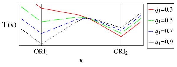
(color online). Replication time curves for differing values of competence q₁. Parameters values: q₂ = 0.7, τ = 1, Δt = 4, D = 10, v = 1.

Equation (6) challenges the assumption that origins are located at minima of T(x). From Eq. (6) the expression for the slope of T near the first origin (for x > 0):

$$T^{\prime }\left(x\right)=\frac{q_1-q_2{s}_1}{v(1-s_1{s}_2)}.$$ (8)

This expression shows that the slope is a function of the competencies q_i of both origins as well as the fork velocity v. For the origin at x = 0 to be a minimum of T(x), we must have T′ > 0 for x > 0, from which we get the condition $q_1>\frac{q_2}{1+q_2}$. This shows that if an origin has low competence compared to its neighbor, it may not be a minimum of T(x), which can be seen in Fig. 1. This phenomenon has been observed in experimental data [4]. Note that if q₁ > 1/2, this condition is always satisfied and a minimum is guaranteed for this two-origin system. In addition, Eq. (8) shows that the fork velocity is not given by the slope of T(x), an assumption widely used in the literature [4].

Figure 1 shows that T(x) has sharp corners at origin locations. The reason for this is that in every cell the forks always start at the same locations (the origins), which causes a discontinuous change in the proportion of left-propagating compared to right-propagating replication forks, which in turn causes the discontinuity in the derivative of T(x) at the origins. In contrast, Fig. 1 shows that the local maximum of T(x) between two origins is a smooth curve. The reason is that in different cells in a population forks meet each other and terminate at different locations on the DNA, because of the stochastic variations in activation times. This reasoning suggests that the shape of the maxima of T could be used to infer information about the width Δt of the activation time distribution. We expect that sharp maxima should correspond to forks meeting within a narrow time window, and consequently a small value of Δt; conversely, a broad maximum corresponds to a high Δt. This can be seen in Fig. 2, where T(x) is plotted for various values of Δt. In order to investigate this more quantitatively, we use the modulus of the second derivative of T(x) at the maxima to measure how broad the maxima is—low values of |T″| correspond to broad peaks. We now use Eq. (6) to find the relationship between |T″| and the origin parameters. At the maximum of T(x), we find

$$\mid T^{\prime \prime }\mid =\frac{4q_1{q}_2\sqrt{1-\mid \frac{1}{q_2}-\frac{1}{q_1}\mid }}{v^2\Delta t(1-s_1{s}_2)}.$$ (9)

Thus |T″| is inversely proportional to Δt. Notice also that |T″| does not depend on τ, which means it is independent of the origins’ average activation times. This expression can be used to calculate Δt from an experimental replication time profile T(x), if the origin competencies and the fork velocity are known. This is a very useful result because it allows the determination of a quantity characterizing stochastic properties of the system Δt from T(x), which is defined by a population average. This is valuable because experiments to directly measure Δt are technically difficult, and there are few results available [5,6]. We note that this does not require assuming that all cells in the population are synchronized, since in each individual cell in an asynchronous population, the statistics of the relative activation times of origins remain unaltered [8].

FIG. 2.

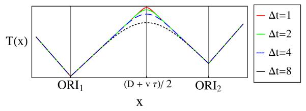
(color online). Replication time curves for different widths of the activation time window.

Equation (9) was obtained using a simple uniform distribution for p_i(t). However, we expect it to be a good approximation for any single-peaked distribution function p_i(t), since Eq. (9) only involves the second moment (the variance) of the distribution, and the replication dynamics are mostly determined by the average activation time and the width of the activation distribution—the first and second moments of p_i(t). To test this assumption we used Eqs. (1)-(6) to numerically compute T(x) for pairs of origins with either a Gaussian or a skewed distribution that lead to sigmoidal cumulative distributions [14]. Choosing parameters such that all these distributions have the same mean and variance, we find that in all cases T″ never differs between distributions by more than 10%.

Despite the fact that we have been considering a hypothetical two-origin chromosome, we expect Eq. (6) to be a good approximation for chromosomes with many origins when two neighboring origins are relatively isolated from other origins. To test this, we looked at experimental data [4] for S. cerevisiae chromosome X, specifically the region containing origins ARS1012/13 and ARS1014 (Fig. 3). The smoothness of the curve—ignoring the fluctuations caused by experimental noise—is direct evidence for stochastic origin activation, in agreement with other results [5,6]. We fitted a parabola through the data points and from this determined the value of |T″|. Using Eq. (9) we estimate the value of Δt as 10.8 min [19]. This value is in agreement with the limited number of single cell measurements that have been made at other S. cerevisiae origins [6].

FIG. 3.

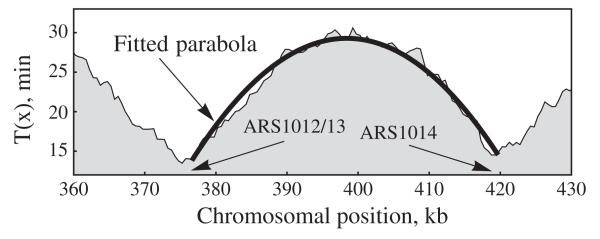
Replication time curves [4] for S. cerevisiae chromosome X with a fitted parabola [375–420 kilobase pairs (kb)].

References

- [1].Nieduszynski CA, Knox Y, Donaldson AD. Genes Dev. 2006;20:1874. doi: 10.1101/gad.385306. [DOI] [PMC free article] [PubMed] [Google Scholar]
- [2].Nieduszynski CA, Hiraga SAP, Benham CJ, Donaldson AD. Nucleic Acids Res. 2007;35:D40. doi: 10.1093/nar/gkl758. [DOI] [PMC free article] [PubMed] [Google Scholar]
- [3].Blow JJ, Gillespie PJ. Nat. Rev. Cancer. 2008;8:799. doi: 10.1038/nrc2500. [DOI] [PMC free article] [PubMed] [Google Scholar]
- [4].Raghuraman MK, Winzeler EA, Collingwood D, Hunt S, Wodicka L, Conway A, Lockhart DJ, Davis RW, Brewer BJ, Fangman WL. Science. 2001;294:115. doi: 10.1126/science.294.5540.115. [DOI] [PubMed] [Google Scholar]
- [5].Tuduri S, Tourriere H, Pasero P. Chrom. Res. 2010;18:91. doi: 10.1007/s10577-009-9098-y. [DOI] [PubMed] [Google Scholar]
- [6].Kitamura E, Blow JJ, Tanaka TU. Cell. 2006;125:1297. doi: 10.1016/j.cell.2006.04.041. [DOI] [PMC free article] [PubMed] [Google Scholar]
- [7].Friedman KL, Brewer BJ, Fangman WL. Genes Cells. 1997;2:667. doi: 10.1046/j.1365-2443.1997.1520350.x. [DOI] [PubMed] [Google Scholar]
- [8].de Moura APS, Retkute R, Hawkins M, Nieduszynski CA. Nucleic Acids Res. 2010;38:5623. doi: 10.1093/nar/gkq343. [DOI] [PMC free article] [PubMed] [Google Scholar]
- [9].Lygeros J, Koutroumpas K, Dimopoulos S, Legouras I, Kouretas P, Heichinger C, Nurse P, Lygerou Z. Proc. Natl. Acad. Sci. U.S.A. 2008;105(12):295. doi: 10.1073/pnas.0805549105. [DOI] [PMC free article] [PubMed] [Google Scholar]
- [10].Spiesser T, Klipp E, Barberis M. Mol. Genet. Genomics. 2009;282:25. doi: 10.1007/s00438-009-0443-9. [DOI] [PMC free article] [PubMed] [Google Scholar]
- [11].Sekedat MD, Fenyö D, Rogers RS, Tackett AJ, Aitchison JD, Chait BT. Mol. Syst. Biol. 2010;6:353. doi: 10.1038/msb.2010.8. [DOI] [PMC free article] [PubMed] [Google Scholar]
- [12].Hyrien O, Goldar A. Chrom. Res. 2010;18:147. doi: 10.1007/s10577-009-9092-4. [DOI] [PubMed] [Google Scholar]
- [13].Luo H, Li J, Eshaghi M, Liu J, Karuturi RKM. BMC Bioinf. 2010;11:247. doi: 10.1186/1471-2105-11-247. [DOI] [PMC free article] [PubMed] [Google Scholar]
- [14].Yang SC-H, Rhind N, Bechhoefer J. Mol. Syst. Biol. 2010;6:404. doi: 10.1038/msb.2010.61. [DOI] [PMC free article] [PubMed] [Google Scholar]
- [15].Jun S, Bechhoefer J. Phys. Rev. E. 2005;71:011909. doi: 10.1103/PhysRevE.71.011909. [DOI] [PubMed] [Google Scholar]
- [16].Kolmogorov A. Izv. Akad. Nauk. SSSR. 1937;1:335. [Google Scholar]
- [17].Andrienko YA, Brilliantov NV, Krapivsky PL. Phys. Rev. A. 1992;45:2263. doi: 10.1103/physreva.45.2263. [DOI] [PubMed] [Google Scholar]
- [18].Al-Mahboob A, Fujikawa Y, Sadowski JT, Hashizume T, Sakurai T. Phys. Rev. B. 2010;82:235421. [Google Scholar]
- [19].Parameter values used were q1 = 0.74, q2 = 0.78 and v = 1/9 kb/min, estimated in [8].