Mathematical modeling of genome replication

Abstract

Eukaryotic DNA replication is initiated from multiple sites on the chromosome, but little is known about the global and local regulation of replication. We present a mathematical model for the spatial dynamics of DNA replication, which offers insight into the kinetics of replication in different types of organisms. Most biological experiments involve average quantities over large cell populations (typically >10⁷ cells) and therefore can mask the cell-to-cell variability present in the system. Although the model is formulated in terms of a population of cells, using mathematical analysis we show that one can obtain signatures of stochasticity in individual cells from averaged quantities. This work generalizes the result by Retkute et al. [Phys. Rev. Lett. 107, 068103 (2011)] to a broader set of parameter regimes.

I. INTRODUCTION

DNA replication, the process during which cells’ genetic information is duplicated, is one of the most fundamental processes in biology. Eukaryotic cells regulate the replication of their genomes in a highly complex manner: it is vital that chromosomal replication be completed before cell division takes place, in order to pass full and accurate genetic information to the daughter cells.

Cell cycle progression in eukaryotic organisms consists of four morphologically distinct phases: a gap phase (G1) during which a cell grows, followed by the DNA synthesis (S) phase, when the cell’s genome is duplicated, a second gap phase (G2), and the mitosis (M) phase, when the cell divides into two [1]. The duration of each of these phases varies from organism to organism, but in all eukaryotes chromosome replication occurs during the S phase and is initiated at specific locations on the chromosome called replication origins. When an origin is activated, two replication forks are formed, which travel on the chromosome in opposite directions. The number of origins varies depending on species and cell type; for example, most bacterial genomes are replicated from a single origin. The size of eukaryotic genomes necessitates the use of multiple origins to ensure timely and complete replication prior to cell division. The use of multiple origins requires tight regulation of origin activity to ensure that sufficiently many origins are activated, but that no origin is activated more than once in a single round of genome replication. This is achieved by the mechanism of licensing of replication origins. This consists of binding of a series of specific protein complexes at origin sites in the DNA, followed by the loading of pairs of Mcm2-7 molecules. If in a given cell licensing of a certain origin is not completed by the time the S phase starts, that origin is unable to function [2]. Also regulated are the number of origins that are activated in a given S phase and timing of the replication of specific regions on a chromosome [3].

There has been much interest recently in the mathematical modeling of DNA replication [4–15]. Two different modeling approaches have been used: simulations to capture the replication dynamics at a single cell level [8–12], and probabilistic models that characterize the dynamics of replication at a population level [5,7,13–15]. Although valuable insights have been gained from previous works on mathematical modeling, they ignore the possibility that origins can fail to license, and we will show that this has a crucial effect on the system’s dynamics [4,5]. In addition, most of the existing models are numerical.

In this work, we analyze an analytical model of eukaryotic DNA replication which fully takes into account the stochastic nature of both the licensing process and origin activation [5]. We start by formulating a general model for organisms with multiple chromosomes and multiple origins; then we analyze in detail the kinetics of replication for an idealized chromosome with two origins, where the most important features of the replication dynamics can be studied in its simplest nontrivial case. We focus on quantities which are of biological interest: replication profiles, average number of active origins, replicon sizes, and others; and we derive explicit analytical expressions for them.

Genome replication has been comprehensively studied in the model organism Saccharomyces cerevisiae (brewer’s yeast). High-throughput experiments have allowed the measurement of replication times as a function of chromosomal position for the whole genome [16]. These methods yield average replication times at distinct chromosomal positions, over large cell populations (typically >10⁷ cells), and therefore can mask the cell-to-cell variability present in the system [17]. To date single cell and single molecule studies are not able to measure the kinetics of whole genome replication [17,18]. The low abundance of the molecules involved in triggering origin activation strongly suggests that origins have stochastic activation times [19], with origins having different relative activation probabilities [20].

Replication origins in eukaryotic organisms must successfully complete the process of licensing in order to be able to replicate during the S phase. Licensing involves a number of orchestrated binding events between origin sites and molecules, some of which are present in low numbers in the cell. Once the S phase starts, no further licensing is allowed, so each origin has a relatively short time window in which to complete licensing. This suggests that a given origin will not manage to complete licensing in every cell within a population before the onset of the S phase, due to inhomogeneities in the abundance of key molecules caused by stochasticity in their expression. We anticipate that different origins will have different licensing efficiencies, due to known differences in affinities to the various species involved in licensing [21], as well as stochasticity in the chemical dynamics of licensing. This leads us to the concept of origin competence [4], which is the probability that a given origin in a population will finish the licensing process before the S phase, and is thus eligible for originating replication forks. The competence of an origin is hard to measure directly, although plasmid replication efficiency experiments suggest that many origins in yeast have low competence, making the concept relevant to the study of the dynamics of replication. The concept of competence introduces an additional parameter to each origin in a chromosome, which has the technical disadvantage that it makes parameter estimation from data somewhat problematic, as discussed in [4]. Despite this, we feel there are compelling biological reasons to take this effect into account and investigate its consequence for DNA replication dynamics; this is one of the main goals of this work.

We note that this idea of origins with less than 100% competence is compatible with the hypothesis that origins have a probability distribution of having different numbers of Mcm2-7 molecules, which is proposed in [20] to determine their activation times. But any mechanism generating a stochastic distribution of Mcm2-7 numbers in an origin will have a nonzero probability of not having a pair of Mcm2-7 molecules in any particular origin; this corresponds exactly to the origin having failed to license, and therefore having a competence below 100%.

We notice that the dynamics of DNA replication has many similarities with the process of nucleation, and some models of DNA replication [7,14] are closely related to Kolmogorov’s classical model of nucleation [22]. The model we propose here can be regarded as an inhomogeneous model of nucleation with quenched disorder, where nucleation starts at specific sites. Inhomogeneous models of nucleation have been studied in the context of statistical physics and have relevance to surface science and other areas [23,24].

II. THE MODEL

In our model we consider a chromosome with N origins, where each origin i is defined by the following parameters: its chromosomal position x_i; the probability q_i that the origin achieves licensing (in a given cell within a population), and is thus capable of activating, i.e., competence; and the activation time probability distribution p_i(t), which is the probability density of origin i activating and starting bidirectional replication forks at time t [4]. Since an origin may not be competent in every cell within the population, in general q_i < 1, and p_i satisfies

$${\int }_{-\infty }^{+\infty }{p}_i\left(t\right)\mathit{dt}=q_i.$$

The fundamental quantity from which all statistical properties of this system can be calculated is the probability density P(x,t), defined such that P(x,t)dt is the probability that chromosomal position x is replicated between times t and t + dt. If only origin i were present, P would be given by P(x,t) = p_i(t – |x – x_i|/ν), where ν is the fork velocity, which we assume to be a constant.

In the presence of all N origins, the calculation of P(x,t) is complicated by the fact that position x can be replicated by forks originated from any of the origins [4,14]. Let us assume that position x is replicated between times t and t + dt by a fork from origin i. This requires that (i) origin i activated at time t – |x – x_i|/ν, so that the fork arrives at x at time t; and (ii) all other origins j ≠ i either have not activated or they have activated but their forks would arrive at x later than t. This allows us to account for passive replication—i.e., an origin is inactive due to replication by a fork that originated at another origin The probability density for event (i) is

$$p_i(x,t)=p_i(t-\mid x-x_i\mid ∕v),$$ (1)

and the probability for event (ii) is

$$Q_i(x,t)=\prod _{j\ne i}{M}_j(x,t),$$ (2)

where M_i is the probability that a fork from origin i arrives later than t, or fails to activate:

$$M_i(x,t)=s_i+{\int }_t^{+\infty }{p}_i(x,\tau )d\tau ,$$ (3)

where s_i = 1 – q_i is the probability of origin i not being competent. Therefore, the probability density P_i(x,t) that position x is replicated by origin i at time t is

$$P_i(x,t)=p_i(x,t)Q_i(x,t).$$ (4)

Finally, the probability density that position x is replicated at time t, irrespective of which origin the fork started from, is [5]

$$P(x,t)=\sum _{i=1}^N{P}_i(x,t).$$ (5)

Using Eq. (5), expressions for various quantities of biological interest can be found. We notice here that similar expressions have been derived before for the case where all the origins are 100% competent [14].

III. GENERAL RESULTS FOR THE MODEL

Now we will derive expressions for important quantities characterizing the replication dynamics, which are of great interest to biologists working in this area: the mean replication time; the efficiency of origins, that is, in what fraction of cells a given origin has activated in a round of replication; the fraction f of total DNA replicated (or the relative DNA content) at any given time in the S phase; the rate of origin initiation in a population; the number of replication forks and active origins as a function of time; the probability of fork termination and how it depends on the chromosomal position; and the interorigin distance distribution between active origins. All these quantities are derived below from the fundamental expression Eq. (5).

A. Mean replication time

One of the most important quantities in the area of DNA replication biology is the replication profile, which is the mean replication time T(x) at the chromosomal position x; here the average is over a large population of cells, which is the typical situation in experiments. There are a number of techniques for obtaining whole-genome replication profiles, such as the density transfer method or by measuring relative DNA copy number using microarray [16,25] or next generation sequencing [26,27] techniques. In the biological literature, the term “replication profile” has a number of different but related meanings: mean replication time, mean percentage replicated, mean copy number at a chromosomal position; or the so-called S:G1 ratio, where cells in the G1 and S phases of the cell cycle are sorted and numbers of cells in both phases are compared for each sequence [27–33]. All of those quantities are closely related to the mean replication time T(x), and they contain essentially the same information. Therefore in this paper the term “replication profile” will mean T(x).

From Eq. (5), we can write the mean replication time as

$$T\left(x\right)=\frac{1}{1-{\prod }_{i=1}^n{s}_i}{\int }_{-\infty }^{+\infty }tP(x,t)\mathit{dt},$$ (6)

where the normalization factor $1-{\prod }_{i=1}^n{s}_i={\int }_{-\infty }^{+\infty }P(x,t)\mathit{dt}$ is the that at least one of the origins probability will activate. In Eq. (6) we are thus excluding the situation where all origins simultaneously fail from the definition of the average; the probability of this happening is very remote in real cells. The probabilities will be defined in this way in all the remaining expressions in this paper.

The replication profile ([T(x) curves] has been measured in a number of organisms. However, caution is required when interpreting T(x) curves. In some of the biological literature T(x) curves are used to directly infer origin parameters [16]. For example, it is widely accepted that the values of T at x_i are the average activation times of origins. However, Eq. (6) shows that T(x) is determined collectively by all origins [4,5], which suggests that simple interpretations of T(x) are likely to be misleading. This issue will be discussed in more detail in Sec. VII.

B. Fraction of DNA replicated

The fraction of cells in a population which have position x on the chromosome replicated by time t can be calculated by integrating the probability P(x,t) with respect to t [5]:

$$m(x,t)=\frac{1}{1-{\prod }_{i=1}^n{s}_i}{\int }_{-\infty }^{t}P(x,\tau )d\tau .$$ (7)

The higher the value of the fraction replicated, the earlier the chromosome position replicates on average during the S phase [16].

Replication dynamics has also been studied by measuring the copy number change by differentiating between replicated and nonreplicated stages of the cell cycle [25,27]. The copy number C(x,t) of the position on the genome at a particular time t is given by

$$C(x,t)=m(x,t)+1.$$ (8)

A twofold increase in copy number is required as the cell progresses from the G1 to the G2 phase.

A relationship between mean copy number $\stackrel{‒}{C}\left(x\right)$ and mean replication time T(x) for the S phase which starts at time T₁ and finishes at time T₂:

$$\stackrel{‒}{C}\left(x\right)=\frac{T_2-T\left(x\right)}{T_2-T_1}+1;$$ (9)

for details see Appendix A.

The replicated fraction f(t) of a genome of length L is given by the average over the whole length of the chromosome of the probability that a piece of DNA has replicated by time t:

$$f\left(t\right)=\frac{1}{L}{\int }_0^{L}m(x,t)\mathit{dx}.$$ (10)

As the population of cells enters into the S phase and replication starts, the chromosomal content is equal to one copy of the genome, and the replicated fraction f(t) is 0. As replication progresses, f(t) increases and towards the end of the S phase the DNA content doubles, ensuring a full complement of DNA for each daughter cell. By measuring the fraction of replicated DNA as a function of time, it is possible to determine the rate of total DNA synthesis during the cell cycle [34].

Figure 1(a) shows the simulated replicated fraction for a virtual chromosome with a length 100 kilobase pairs (kb) with ten origins periodically positioned along a chromosome. In this example, each origin has a Gaussian activation distribution with a mean of 15 min and a standard deviation of 5 min. We see that the fraction of DNA replicated as a function of time has a sigmoidal shape.

FIG. 1.

Results for a virtual chromosome of length 100 kb with ten origins periodically positioned along the chromosome. Origin activation follows a Gaussian distribution with a mean of 15 min, a standard deviation of 5 min, and a fork velocity 1.5 kb/min. (a) Fraction of replicated DNA f(t), (b) rate of origin initiation g(t), and (c) initiation rate I(t).

C. Rate of origin initiation

The probability density of a single isolated origin i activating and starting bidirectional replication forks at time t is p_i(t) (Sec. II). Any given origin i can activate only if forks from neighbor origins j ≠ i arrive at position x_i later than time t, or fail to activate, and this probability is given by ${\prod }_{j\ne i}{M}_j(x_i,t)$, with M_j defined by Eq. (3). Then the rate of origin initiation g(t) is defined as the sum over all origins of the probability densities of the origins activating at a time t:

$$\mathsf{g}\left(t\right)=\frac{1}{1-{\prod }_{i=1}^n{s}_i}\sum _{i=1}^N{p}_i\left(t\right)\prod _{j\ne i}{M}_j(x_i,t).$$ (11)

The importance of this quantity lies in the fact that in a large population of cells, the number of origins activating in a small time window (t,t + dt) is proportional to g(t); hence the term “rate” used above.

Population-averaged measurements of replication initiations per time unit per unit length of unreplicated DNA have been obtained for a number of organisms, including S. cerevisiae, Schizosaccharomyces pombe, Drosophila melanogaster, Xenopus laevis, and Homo sapiens [34,35]. All profiles have been observed to possess a strikingly similar shape: increasing during the first half of the S phase and then decreasing before the end of the S phase.

The initiation rate, i.e., the rate of origin initiations per time unit per unit length of unreplicated DNA, is obtained by dividing Eq. (11) by the chromosome length L and by the fraction of DNA still unreplicated at time t [obtained from Eq. (10)]:

$$I\left(t\right)=\frac{\mathsf{g}\left(t\right)}{L[1-f(t\left)\right]}.$$ (12)

To test if the model reproduces the behavior of the initiation rate observed in the experiments described in [35], we have applied Eqs. (11) and (12) to the virtual chromosome described in Sec. III B. We consider a virtual chromosome with a length of 100 kb replicated from ten origins periodically positioned along the chromosome; each origin has a Gaussian activation distribution function with a mean of 15 min and a standard deviation of 5 min. The general shape of the curve predicted for the initiation rate per time unit per unreplicated unit of DNA [I(t); Fig. 1(c)] is in good agreement with the experimental results [35]. In the case we have analyzed, the initiation rate I(t) increases during the first 4/5 of the S phase and then declines for the last 1/5 of the S phase. This late decrease is due to the rate of the origin initiation function g(t) reaching its maximum just after mid-S-phase (at 14 min). The end of the S phase is the time at which the fraction of DNA replicated, f(t), reaches 1 (at 25 min).

D. Origin efficiency and average number of active origins

The efficiency of an origin i is the fraction of cells in a population that actually activated that origin in any given S phase [36]. In any given cell, not all origins will be activated during the S phase; for example, in some mammalian cells most origins are used in less than 10% of cell cycles [26].

The efficiency of origin i is the probability that origin i activates at any time, and is therefore given by the integral of the probability that the ith origin initiates between times t and t + dt multiplied by the probability that none of the other origins has replicated position x_i before time t [4,14]:

$$e_i=\frac{1}{1-{\prod }_{i=1}^N{s}_i}{\int }_{-\infty }^{\infty }{p}_i\left(t\right)\prod _{j\ne i}{M}_j(x_i,t)\mathit{dt}.$$ (13)

It has been observed in experiments that the efficiency of origins depends heavily on the distance and timing of activation of neighboring origins [37]. This is seen directly from Eq. (13), where the term ${\prod }_{j\ne i}{M}_j(x_i,t)$ encodes the influence of other origins on the chromosome.

Another quantity describing the collective dynamics of DNA replication is the average number n_O of active origins, that is, on average how many origins have activated in a cell within a population. The presence of multiple origins creates redundancy and the average number of activated origins will be less than the total number of origins present on a chromosome.

The average number of active origins is readily obtained from the origin initiation rate given by Eq. (11):

$$n_o={\int }_{-\infty }^{\infty }\mathit{g}\left(t\right)\mathit{dt}.$$ (14)

Applying Eq. (11) to Eq. (14) and using Eq. (13), we can relate the average number of active origins to origin efficiencies:

$$n_o=\sum _{i=1}^n{e}_i$$ (15)

Figure 2 shows the probability distribution for a number of activated origins on S. cerevisae chromosome VI, based on origin efficiencies determined experimentally [19] and calculations based on normal activation distribution and parameter values from [4]. The average number of active origins n_O on chromosome VI, calculated using Eq. (15) based on experimental data and parameter estimation, gave 3.8 and 3.6 origins per cell cycle, respectively.

FIG. 2.

Probability distribution for a number of activated origins on S. cerevisae chromosome VI: experimental results from [19] (black full circles) and calculations based on parameter values from [4] (gray empty circles).

E. Describing the dynamics of replication forks

As replication progresses through the S phase, replication forks originate at activated origins, and disappear when two forks moving in opposite directions in the chromosome collide. The average number of forks moving at some time t is a quantity that can yield valuable insights into the replication dynamics. If there were only a single fork moving in the chromosome, the rate df(t)/dt of replication would be simply ν, the fork velocity; n_f forks thus correspond to a replication rate of n_fν, which leads to the expression

$$n_f\left(t\right)=\frac{1}{v}\frac{\mathit{df}\left(t\right)}{\mathit{dt}},$$

where f(t) is the fraction of replicated DNA at time t. This expression was also derived for DNA replication in X. laevis [38]. By applying Eqs. (7) and (10) in above equation we have

$$n_f\left(t\right)=\frac{1}{v(1-{\prod }_{i=1}^n{s}_i)}{\int }_0^{L}P(x,t)\mathit{dx},$$ (16)

where L is the length of the chromosome.

The direction of replication fork movement can be analyzed using a distribution for the proportion of left moving forks at each position x:

$$\begin{array}{cc}\hfill n_{\text{left}}\left(x\right)=& \frac{1}{1-{\prod }_{i=1}^n{s}_i}{\int }_{-\infty }^{\infty }\sum _{i=1}^N\mathcal{I}(x<x_i)p_i(x,t)\hfill \\ \hfill & \times \prod _{j\ne i}{M}_j(x,t)\mathit{dt},\hfill \end{array}$$ (17)

where $\mathcal{I}\left(X\right)$ is the indicator function, which takes a value equal to 1 if the condition X is satisfied and 0 otherwise.

Figure 3(a) shows the probability distribution for the proportion of leftward traveling forks at position x for S. cerevisae (chromosome VI), computed using Eq. (17), with origin parameters estimated in [4]. All regions except for the start and the end of the chromosome are replicated by both leftward and rightward moving forks.

FIG. 3.

Probability distribution for (a) the proportion of left moving forks, (b) fork termination at position x on S. cerevisae chromosome VI based on Eq. (16), and (c) histogram of fork termination sites based on 10⁶ Monte Carlo simulations. Parameter values from [4].

The difference between the proportion of right and left moving forks gives the average fork polarity f_pl(x). The average fork polarity is the product of the derivative of the mean replication time and the replication fork velocity [15]:

$$f_{\mathit{pl}}\left(x\right)={\mathit{vT}}^{\prime }\left(x\right).$$

Taking into account that the sum of the proportion of left and right moving forks is equal to 1, this gives the relationship between the proportion of left moving forks and mean replication time:

$$n_{\text{left}}\left(x\right)=\frac{1-{\mathit{vT}}^{\prime }\left(x\right)}{2}.$$

When two forks collide, they both terminate and replisome proteins are released from the DNA molecule. In Escherichia coli termination sites are regulated and fixed, but in eukaryotes termination is less well defined than in bacteria, and specific sites are rare [39].

To find the probability density of termination events at position x and at time t, we first consider any given pair of origins i and j with i < j—so their positions satisfy x_i < x_j. For the forks originating at i and j to terminate exactly at position x at a time t, the following conditions must be met: (a) x must lie between x_i and x_j; (b) i and j must have activated at times $t-\frac{\mid x-x_i\mid }{v}$ and $t-\frac{\mid x-x_j\mid }{v}$, respectively; and (c) the position x must not be replicated by any other origin k, with k ≠ i,k ≠ j, at time t. The total probability density of fork termination at position x and time t is the sum of the termination probabilities for all possible pairs (i,j) satisfying x_i ≤ x ≤ x_j; since i < j, it is enough to consider indices in the sum given by i = 1,…,N and j = i + 1,…,N – 1. Finally, the probability (density) that forks will terminate at x is found by integrating over all times, yielding the expression

$$\begin{array}{cc}\hfill P_{\mathrm{ft}}\left(x\right)=& \frac{1}{\mathcal{N}}{\int }_{-\infty }^{\infty }\sum _{i=1}^N\sum _{j=i+1}^{N-1}\mathcal{I}(x_i\le x\le x_j)\hfill \\ \hfill & \times p_i(x,t)p_j(x,t)\prod _{k\ne i,k\ne j}{M}_k(x,t)\mathit{dt},\hfill \end{array}$$ (18)

where $\mathcal{N}$ is a normalization constant.

Figure 3(b) shows the probability distribution of fork termination at position x for S. cerevisae (chromosome VI), computed using Eq. (18), with origins activating according to a normal distribution with mean and variance values estimated in [4]. For a comparison, we have plotted a histogram of fork termination sites based on 10⁶ Monte Carlo simulations [Fig. 3(c)], the solution based on Eq. (18) agrees with the simulation results within statistical limits.

F. Distribution of distances between active origins

The distribution of distances between active origins (between origins that have actually activated) in a population of cells is an important quantity for biology. Its importance is related to the fact that the stochastic nature of origin activation can result in large distances between active origins, with the consequence that sections of the genome would take too long to replicate; this can result in portions of the genome remaining unreplicated when cells enter the M phase [40] or causing instability in fragile sites [41].

For organisms such as yeast where the replication origins have fixed positions in any given chromosome, the inter-active-origin distance can assume only a discrete set of values. For example, about 120 early inter-active-origin distances in fission yeast and between 250 and 300 in budding yeast [42] have been observed to have a typical spacing of between 30 and 100 kb [43]. In normal human primary keratinocyte cells, the mean value for inter-active-origin distances is about 124 kb [44].

The distance y_ij between origins i and j is equal to y_ij = |x_i – x_j|, where x_i is the position of origin i and x_j is the position of origin j. Our goal is to obtain an expression for the probability distribution of distances between active origins $\mathcal{P}\left(y\right)$ for the interorigin distance y. Consider first a given origin pair (i,j), with i < j, then the probability density that this particular pair activates in one replication round, and no other origin activates in between them—this event contributes to $\mathcal{P}$ with y_ij. The probability density that origin i activated at time t and neighboring origins on the left either have not activated or they have activated but their forks would arrive at x_i later than t, is given by p_i(t) $p_i\left(t\right){\prod }_{k=1}^{i-1}{M}_k(x_i,t)$. The probability density that origin j has activated at time t and neighboring origins on the right either have not activated or they have activated but their forks would arrive at x_j later than t; this is given by $p_j\left(t\right){\prod }_{k=j+1}^N{M}_k(x_j,t)$. Since y_ij = y_ji it is sufficient to consider origin pairs with indices i and j with ranges given by i = 1,…,N and j = i + 1,…,N – 1. Further, if i and j are such that j – i > 1, i.e., these origins are not adjacent, we need to ensure that all origins k lying between them (i < k < j) will not activate at all (otherwise there would be an origin activating between i and j, and this would split the interval [x_i,x_j] into two); this probability is equal to ${\prod }_{k=i+1}^{j-1}{M}_k(x_k,t)$. The probability density function for inter-active-origin distances is given by the integral over all times of the product of these probabilities:

$$\begin{array}{cc}\hfill P\left(y\right)=& \frac{1}{\mathcal{N}}{\int }_{-\infty }^{\infty }\sum _{i=1}^N\sum _{j=i+1}^{N-1}\mathcal{I}(y=\mid x_i-x_j\mid )\hfill \\ \hfill & \times p_i\left(t\right)p_j\left(t\right)\prod _{k=1}^{i-1}{M}_k(x_i,t)\prod _{k=j+1}^N{M}_k(x_j,t)\hfill \\ \hfill & \times \prod _{k=i+1}^{j-1}{M}_k(x_k,t)\mathit{dt},\hfill \end{array}$$ (19)

where $\mathcal{N}$ is a normalization constant. The probability density function $\mathcal{P}$ takes nonzero values for y equal to distances separating any two origins on the chromosome.

Figures 4(a) and 4(b) show the probability distribution of distances between active origins for S. cerevisae (chromosome VI), computed using Eq. (19) and a histogram for 10⁵ Monte Carlo simulation, with normal activation distribution and parameter values estimated in [4]. Based on this distribution, we calculate that the mean distance between active origins is 55 kb. Whole-genome analysis has shown that the average distance between active replication origins in the S. cerevisiae genome is approximately 58 kb [45]. We note that the distribution of inter-active-origin distances has a long tail; ~4% of cells have an inter-active-origin distance >130 kb. Similar & large inter-active-origin distances have been observed experimentally [45,46]. To prevent under-replication (or delay to cell cycle progression) these large inter-active-origin distances much be replicated prior to cell division. S. cerevisiae cells have about 60 min available to complete DNA replication before cell division starts, i.e. two forks converging at 2 kb/min can potentially replicate 240 kb during that time; therefore under-replication is unlikely according to our model.

FIG. 4.

Probability distribution of distances between active origins on S. cerevisae chromosome VI: (a) as a solution of Eq. (19), and (b) histogram for 10⁵ Monte Carlo simulation. Parameter values from [4].

IV. PARAMETER REGIMES

We want to use the general theory presented above to study replication dynamics in a simple setting. From now on we focus on the case of a hypothetical linear chromosome with just two origins. We define the chromosomal coordinates so that one of the origins has position x₁ = 0; the other origin has position x₂ = D. We assume that each origin can activate within a time window Δt_i with uniform probability; we will argue later that our conclusions are largely independent of the precise shape of the probability distribution. We select the time axis in such a way that the average activation time of the first origin is 0. The other origin has an average activation time τ, and we assume without loss of generality that τ ≥ 0. Thus the activation time distributions are

$$p_i\left(t\right)=\frac{q_i}{\Delta t_i}\text{if}t\in \left[t_i^{\mathrm{av}}-\frac{\Delta t_i}{2},t_i^{\mathrm{av}}+\frac{\Delta t_i}{2}\right],$$ (20)

where i = 1,2, $t_1^{\mathrm{av}}=0$ and $t_2^{\mathrm{av}}=\tau$, and p₁ and p₂ are set to zero outside the stated intervals.

Using Eqs. (6) and (20), we canwrite analytical expressions for the probability density P(x,t) and other quantities of interest. From Eqs. (20) and (5), P(x,t) vanishes outside the intervals $I_1=[I_1^l,I_1^u]$ and $I_2=[I_2^l,I_2^u]$ given by

$$\begin{array}{cc}\hfill I_i^l=& \frac{\mid x_i-x\mid }{v}+t_i^{\mathrm{av}}-\frac{\Delta t_i}{2};\hfill \\ \hfill I_i^u=& \frac{\mid x_i-x\mid }{v}+t_i^{\mathrm{av}}+\frac{\Delta t_i}{2}.\hfill \end{array}$$

A. States of replication

There are six possible states of the replication at each position x on the chromosome, defined by the order in which forks from the two origins can replicate x. These are summarized in Fig. 5, where each position has a probability to be replicated at any time t by origin 1, origin 2, or by either origin depending on the distance from each origin and other parameters. The different possibilities are denoted by “states” A to F, as defined in Fig. 5.

FIG. 5.

A particular position along a chromosome in different cells can be replicated by forks from origin 1 (light gray), origin 2 (dark gray), or either origin (black). The order in which this happens (indicated in A–F above) as time progresses from left to right defines the possible states of replication.

State A corresponds to the situation where forks from origin 1 arrive at x before any fork coming from origin 2; if the competence q₁ of origin 1 is equal to 1, then this position is completely replicated by the first origin. For q₁ < 1, x is replicated by origin 2 only when origin 1 fails to activate. The replication probability density P(x,t) is given in this case by

$$P(x,t)=\{\begin{array}{cc}\hfill \frac{q_1}{\Delta t_1}\hfill & \hfill \text{if}t\in I_1,\hfill \\ \hfill \frac{s_1{q}_2}{\Delta t_2}\hfill & \hfill \text{if}t\in I_2,\hfill \\ \hfill 0\hfill & \hfill \text{otherwise}.\hfill \end{array}\phantom{\}}$$ (21)

In similar manner, state B corresponds to forks from origin 2 arriving at x before forks from origin 1:

$$P(x,t)=\{\begin{array}{cc}\hfill \frac{q_2}{\Delta t_2}\hfill & \hfill \text{if}t\in I_2,\hfill \\ \hfill \frac{s_2{q}_1}{\Delta t_1}\hfill & \hfill \text{if}t\in I_1,\hfill \\ \hfill 0\hfill & \hfill \text{otherwise}.\hfill \end{array}\phantom{\}}$$ (22)

For the states C and D, there is an overlapping time window, when forks originating at either of the origins can get to x first. States E and F show that the time window where x is replicated by forks originating at one of the origins is contained in the time window of the other fork; this latter state is possible only if Δt₁ ≠ Δt₂.

If we denote by [t_l,t_u] the overlapping time window in cases C–F, then the replication probability densities for these four cases are given by the expression below, with i and j having different meanings for each state: C (i = 1,j = 2), D (i = 2,j = 1), E (i = j = 1), and F (i = j = 2):

$$P(x,t)=\{\begin{array}{cc}\hfill p_i\hfill & \text{if}y\in [I_i^l,t_l],\hfill \\ \multicolumn{2}{c}{p_1({\int }_t^{I_2^u}{p}_2\mathit{dt}+s_2)+p_2({\int }_t^{I_1^u}{p}_1\mathit{dt}+s_1)}\\ \hfill \hfill & \text{if}t\in [t_l,t_u],\hfill \\ \hfill p_j\hfill & \text{if}t\in [t_u,I_j^u],\hfill \\ \hfill 0\hfill & \text{otherwise}.\hfill \end{array}\phantom{\}}$$ (23)

Expressions for t_l and t_u for the different states are given in the table below:

State	tl	tu
C	$\frac{\mid D-x\mid }{v}+\tau -\frac{\Delta t_2}{2}$	$\frac{\mid x\mid }{v}+\frac{\Delta t_1}{2}$
D	$\frac{\mid x\mid }{v}-\frac{\Delta t_1}{2}$	$\frac{\mid D-x\mid }{v}+\tau +\frac{\Delta t_2}{2}$
E	$\frac{\mid D-x\mid }{v}+\tau -\frac{\Delta t_2}{2}$	$\frac{\mid D-x\mid }{v}+\tau +\frac{\Delta t_2}{2}$
F	$\frac{\mid x\mid }{v}-\frac{\Delta t_1}{2}$	$\frac{\mid x\mid }{v}+\frac{\Delta t_1}{2}$

From the above table we can see that the state changes as position is changed along the chromosome. Based on these states it is possible to classify the replication dynamics into a number of parameter regimes. Figure 6 shows such regimes for Δt₁ = Δt₂ = Δt and Δt₁ ≠ Δt₂. In the first case [Fig. 6(a)], the number of parameters is reduced and we can look at the full dependencies between τ, Δt, D, and ν. When Δt₁ ≠ Δt₂, we will look at regimes for a few values of τ, Δt₁, and Δt₂ [Figs. 6(b)–6(d)].

FIG. 6.

Plots showing parameter regime diagrams based on the spatiotemporal dynamics of replication: gray areas indicate where the activation time distribution of origin 1 or 2 has nonzero values, and dark gray regions are where distributions for the two origins overlap. (a) Regimes for Δt₁ = Δt₂. (b) Some of the regimes for Δt₁ ≠ Δt₂. (c) Regimes for variable Δt₁ (fixed value of Δt₂ ≪ D/ν) and Δt₂ (fixed value of Δt₁ ≪ D/ν) for τ < D/ν. (d) Regimes for variable Δt₁ (fixed value of Δt₂ ≪ D/ν) and Δt₂ (fixed value of Δt₁ ≪ D/ν) for τ > D/ν. Parameter values for (c) and (d) where replication dynamics undergoes changes are given in Appendix C.

B. Regimes for Δt₁ = Δt₂

In total there are five regimes (depending on the relative values of τ, Δt, D, and ν) that differ in the dynamics of how the chromosome is replicated [shown in Fig. 6(a)]. For regime R₁ only state A occurs for the whole chromosome.

Most relevant to biological systems is regime R₂, since this is the case for many pairs of origins in real chromosomes. In this regime, the condition τ + Δt < D/ν is satisfied, meaning that origins activate at a similar time and the variations in the activation time Δt are small enough that a fork from one origin can replicate the other origin only if that origin is not competent. Regime R₂ is formed from states A, B, C, and D. Changes occur at positions $x=\frac{1}{2}[D+v(\tau -\Delta t\left)\right]$] (from A to C), $x=\frac{1}{2}(D+v\tau$) (from C to D), and $x=\frac{1}{2}[D+v(\tau +\Delta t)$] (from D to B).

Regime R₂ describes the situation where two origins are sufficiently apart that they are not passively replicated by each other. It is quite common, however, to find two origins located close to each other in a chromosome, such that the condition τ + Δt < D/ν is violated. In this case, regimes other than R₂ describe the replication dynamics of the system.

In regime R₃, in some cells origin 2 actives just before forks from origin 1 arrive at position x = x₂ = D and in some cells both origins compete to replicate positions on the right of $x=\frac{1}{2}[D+v(\tau -\Delta t)$]. At this point the behavior changes from state A to C.

For regime R₄ state A occurs up to position $x=\frac{1}{2}[D+v(\tau -\Delta t)$], then it changes to state C. In a similar way, regime R₅ changes from state C to state D at position $x=\frac{1}{2}(D+v\tau )$. More details on the dynamics of replication for different sets of parameters are shown in Fig. 6(a).

For a fixed value of Δt < D/ν, as the difference in average activation time between origins, τ, increases, the replication dynamics undergoes the following changes:

Change	τ	Change	τ	Change	τ
R2 → R3	$\frac{D}{v}-\Delta t$	R3 → R4	$\frac{D}{v}$	R4 → R1	$\frac{D}{v}+\Delta t$

For any fixed τ < D/ν, increasing the width Δt of the activation time distribution leads to change of the regime from R₂ to R₃ at $\frac{D}{v}-\tau$ and from R₃ to R₅ at $\frac{D}{v}+\tau$.

A discussion on regimes for Δt₁ ≠ Δt₂ is given in Appendix C.

V. DYNAMICS OF REPLICATION FORKS

The proportion of left and right moving forks will depend on the properties of the origins and fork velocity, as indicated by Eq. (17). The analytical expression for the proportion of left moving forks, n_left, for regime R₂, is given by Eq. (C1) in Appendix C. In regime R₂ the proportion of left moving forks takes a sigmoidal shape. Figures 7(a), 7(c), and 7(e) show the effect of varying parameters on proportion of left moving forks in regime R₂: as a function of competence q₂ [Fig. 7(a)], as a function of time τ [Fig. 7(c)], and as a function of the width of the activation time distribution Δt₁ = Δt₂ = Δt [Fig. 7(e)]. Parameter values are q₁ = q₂ = 1, τ = 0, Δt₁ = 5, Δ₂ = 5, and ν = 1, if not otherwise stated. The consequences of differences in parameter values can be clearly distinguished: with decreasing competence, the curve is pushed down; increasing τ shifts the curve closer to the second origin; decreasing Δt increases the gradient of the sigmoidal function.

FIG. 7.

The effect of varying parameters on the proportion of left moving forks and fork termination: (a),(b) as a function of competence q₂, (c),(d) as a function of time τ, (e),(f) as a function of width of activation Δt₁ = Δt₂ = Δt, and (g),(h) as a function of width of activation Δt₂. (i) Experimentally measured proportion of left moving forks (gray) [47] on the S. cerevisiae chromosome VII (700–780 kb) with a curve based on Eq. (17) (black) and (j) prediction of the fork termination position probability distribution based on Eq. (D1).

We have also looked at other regimes—in Fig. 7(g) the parameter values Δt₂ = 10 and Δt₂ = 15 correspond to R₇, while Δt₂ = 20 and Δt₂ = 25 correspond to R₉; here q₁ = q₂ = 1, τ = 0 and Δt₁ = 5. Unlike regime R₂, these regimes passive replication of one (R₇) or both (R₉) origins. It can be seen that for these regimes the proportion of left moving forks between the two origins becomes linear with respect to position on the chromosome.

Recently, high-resolution analysis of Okazaki fragment synthesis was performed in S. cerevisiae [47]; this allows determination of the lagging strand proportion and hence the proportion of left moving forks. Figure 7(i) shows the experimentally determined proportion of left moving forks for a part of chromosome VII from 700 to 780 kb (gray lines) with a curve based on Eq. (17) (black) [48]. This demonstrates the close agreement between our model prediction and an independent experimental data set.

VI. RESULTS FOR THE FORK TERMINATION POSITION PROBABILITY DISTRIBUTION

Although the forks all start at the same locations (the origins), they meet each other and terminate at different locations in each cell, because of the stochastic activation times. Only forks traveling in opposite directions between the two origins can collide. This condition limits positions of fork termination to the interval [0; D] (excluding the two ends of the chromosome). (If one of origins is activated much later in time, i.e., the dynamics is in regime R₁, only one origin activates and therefore there are no termination events between the two origins.) The fork termination position distribution will have nonzero values in the areas of the space-time diagram where the probability of that position being replicated by forks from both origins is nonzero. An analytical expression for the fork termination position probability distribution function (PDF) is given in Appendix D.

Figures 7(b), 7(d), 7(f), and 7(h) illustrate the effect of varying the parameters q₂, τ, Δt, and Δt₂. For τ = 0, the maximum of the PDF is at position $x=\frac{D}{2}$ and takes the value $p^{\ast }=\frac{q_1{q}_2(\Delta t_1+\Delta t_2)}{2\Delta t_1\Delta t_2(1-s_1{s}_2)}$. If τ is increased, the maximum moves to the right by $\frac{v\tau }{2}$. The area under the PDF is $\frac{{(\Delta t_1+\Delta t_2)}^2{q}_1{q}_{2}v}{8\Delta t_1\Delta t_2(1-s_1{s}_2)}$ for values $\tau <\frac{D}{v}-\frac{\Delta t_1+\Delta t_2}{2}$; for increasing τ it starts decreasing until zero is reached at $\tau =\frac{2D+v(\Delta t_1+\Delta t_2)}{2v}$.

The biological literature commonly suggests that termination sites are disperse, but there is limited evidence for discrete termination sites [39]. Our model indicates that termination sites have a continuous distribution. Equation (D1) can help identify the most probable positions of fork termination sites on the chromosome. Figure 7(j) shows the prediction of the fork termination position probability distribution for a part of chromosome VII from 700 to 780 kb.

VII. SIGNATURES OF STOCHASTICITY IN REPLICATION PROFILES

In this section we will discuss how information about the stochasticity of the activation times of origins—the width of the activation window—can be obtained from the mean replication time as a function of chromosomal position, T(x). Because the parameter space in the generic case is very big, from now on we will consider only the case Δt₁ = Δt₂ = Δt.

An analytical expression for T(x) for the case where the condition τ + Δt < D/ν is satisfied has been derived [5]. This corresponds to regime R₂ and is the case for many pairs of adjacent origins in real chromosomes. This is valid when the variations in the activation time Δt are small enough that a fork from one origin can replicate the other origin only if that origin is not competent.

A plot of T(x) for various sets of parameters is shown in Fig. 8. We see that T(x) has discontinuous derivatives at the origin locations. This is due to forks originating only at the origin locations; there is a discontinuous change in the proportion of left propagating compared to right propagating forks as one crosses an origin site. At the origins, the mean replication times are [5]

$$\begin{array}{cc}\hfill T\left(x_1\right)=& T\left(0\right)=q_2{s}_1(D∕v+\tau )∕(1-s_1{s}_2);\hfill \\ \hfill T\left(x_2\right)=& T\left(D\right)=(q_1{s}_{2}D∕v+q_2\tau )∕(1-s_1{s}_2).\hfill \end{array}$$ (24)

It is commonly assumed in the replication literature that T(x) has a minimum at an origin, and that the value of this minimum directly gives the average activation time for the origin. However, Eq. (24) shows that this is not the case and, in fact, $T\left(x_i\right)\ge t_i^{\mathrm{av}}$: the mean replication time at an origin location is equal to or greater than the origin’s average activation time. Only when an origin has q_i = 1 can $T\left(x_i\right)=t_i^{\mathrm{av}}$, because if an origin fails to activate in a given cell, the DNA at the origin location will not be replicated until a fork from another origin arrives. This means that T_i is higher for origins that are more likely to fail, as seen directly in Fig. 8(a). Another important conclusion is that even when both origins have the same average activation time (τ = 0), generally we have T(x₁) ≠ T(x₂), also shown in [5]. This is again due to the possibility of origins not activating. Therefore, the origin with the lower minimum of T(x) does not necessarily activate earlier than the other origin: minima of T(x) cannot be used to draw conclusions on the relative activation times of the corresponding origins, as previously assumed [9,16]. The equation for mean replication time shows that in general T(x) at any point depends collectively on the parameters of all origins. However, if an origin is highly competent, early activating, and isolated from other origins, T(x) at that origin’s position will be close to the origin’s average activation time.

FIG. 8.

Replication time curves for (a) differing values of competence q₁; (b) different widths of the activation time window; (c) different values of τ, with position y = x + ντ/2.

The expression for mean replication time, Eq. (24), challenges the assumption that there is a one-to-one correspondence between replication origins and minima of T(x): minima correspond to origin locations, but there may be origins for which there is no peak. The slope of T near the first origin (for x > 0) is [5]

$$T^{\prime }\left(x\right)=\frac{q_1-q_2{s}_1}{v(1-s_1{s}_2)}.$$ (25)

This expression shows that the slope is a function of the competences q_i of both origins as well as the fork velocity ν. For the origin at x = 0 to be a minimum of T(x), we must have T′ > 0 for x > 0, from which we get the condition

$$q_1>\frac{q_2}{1+q_2}.$$ (26)

In a similar way, the slope of T(x) near the second origin (for x < D) is

$$T^{\prime }\left(x\right)=\frac{q_1{s}_2-q_2}{v(1-s_1{s}_2),}$$ (27)

which yields the condition

$$q_2>\frac{q_1}{1+q_1}.$$ (28)

This shows that if an origin has low competence compared to its neighbor, it may not be a minimum of T(x), as illustrated in Fig. 8(a). This phenomenon has been observed in experimental data [16]. Note that if q₁ > 1/2, this condition is always satisfied and a minimum is guaranteed for this two-origin system and this regime. Figure 9 shows values for q₁ and q₂, for which Eqs. (26) and (28) are satisfied, i.e., both origins are local minima in the replication time curve. In addition, Eqs. (25) and (27) show that the fork velocity is not given by the slope of T(x), an assumption widely used in the literature [16].

FIG. 9.

Gray area indicates the sets of competencies q₁ and q₂ for which both origins are local minima in the replication time curve.

In contrast to the discontinuity of T′(x) at the origin locations, the plots of replication time curves show that the local maximum of T(x) between two origins is a smooth curve. The reason is that in different cells in a population forks meet each other and terminate at different locations on the DNA, as has been shown in Sec. VI. This suggests that the shape of the maximum of T(x), when it exists, could be used to infer information about the width of the activation window. We expect that sharp maxima should correspond to forks meeting within a narrow time window; conversely, a broad maximum corresponds to a high time window. This can be seen in Fig. 8(b), where T(x) is plotted for various values of Δt.

In order to investigate this more quantitatively, we use the modulus of the second derivative of T(x) at the maximum to measure how broad the maximum is, because low values of |T′′(x)| correspond to broad peaks. At the maximum of T(x) [5],

$$\mid T^{″}\left(x^{\ast }\right)\mid =\frac{4q_1{q}_2\sqrt{1-\mid \frac{1}{q_1}-\frac{1}{q_2}\mid }}{v^2\Delta t(1-s_1{s}_2)},$$ (29)

where

$$x^{\ast }=\{\begin{array}{c}\frac{D+v\tau }{2}\text{for}{q}_1=q_2;\hfill \\ \frac{D+v\tau }{2}+\frac{v\Delta t}{2}(1-\mid \frac{1}{q_1}-\frac{1}{q_2}\mid )\text{for}{q}_1>q_2;\hfill \\ \frac{D+v\tau }{2}-\frac{v\Delta t}{2}(1-\mid \frac{1}{q_1}-\frac{1}{q_2}\mid )\text{for}{q}_1<q_2.\hfill \end{array}\phantom{\}}$$

Thus |T′′(x*)| is inversely proportional to Δt. Notice also that |T′′(x*)| does not depend on τ, which means it is independent of the origins’ average activation times. Figure 8(c) shows replication time curves for different values of τ, where the position along the chromosome has been shifted by $y=x+\frac{v\tau }{2}$ and replication times are shifted downwards by $\frac{\tau }{2}$. This figure clearly shows that the shape of T(x) near maximum is independent of τ.

Expression (29) can be used to calculate Δt from an experimental replication time profile T(x), if the origin competences and the fork velocity are known. This is a very useful result because it allows the determination of a quantity characterizing stochastic properties of the system, Δt, from T(x), which is defined by a population average. This is valuable because experiments to directly measure Δt are technically difficult [17,18]. We note that this does not require assuming that all cells in the population are synchronized, since in each individual cell in an asynchronous population, the statistics of the relative activation times of origins remains unaltered [4].

VIII. GAUSSIAN AND SKEWED ORIGIN ACTIVATION DISTRIBUTIONS

Although Eq. (29) was obtained using a simple uniform distribution for p_i(t), we expect it to be a good approximation for any single-peaked distribution function p_i(t), since Eq. (29) involves only the second moment (the variance) of the distribution, and the replication dynamics are mostly determined by the average activation time and the width of the activation distribution. So we expect two single-peaked distributions with the same t_av and Δt to have very similar T′′(x).

To test this assumption, we used Eq. (6) to numerically compute T(x) for pairs of origins with Gaussian activation time distribution and with a skewed distribution leading to a sigmoidal cumulative activation time distribution, described by a Hill’s-type function

$$F\left(t\right)=\frac{q\ln 3t_{1∕2}{\left(\frac{t_{1∕2}}{t}\right)}^{\ln 3∕\kappa -1}}{\kappa t^2{\left[1+{\left(\frac{t_{1∕2}}{t}\right)}^{\ln 3∕\kappa }\right]}^2},$$ (30)

where

$$\kappa =\ln \left(\frac{t_w+\sqrt{4t_{1∕2}^2+t_w^2}}{2t_{1∕2}}\right),$$ (31)

as used in Ref. [14].

Figure 10 shows good agreement of the mean replication time and proportion of left moving forks for the three distributions mentioned above. Choosing parameters for which all these distributions have the same mean and variance, we find that in all cases T′′(x) never differs between distributions by more than 10%. This means that Eq. (29) is a very accurate prediction of Δt, regardless of the detailed shape of p_i(t).

FIG. 10.

Plots showing mean replication time (a) and proportion of left moving forks (b) for three different distributions: Uniform distribution ($t_i^{\mathrm{av}}=15$,Δt_i = 8), Gaussian distribution (μ_i 15,σ_i = 2.31), and skewed distribution given by Eq. (30) (t_1/2i = 15.35,t_wi = 2.77), i = 1,2. For all three cases q₁ = 0.9,q₂ = 0.7,ν = 1.

IX. APPLICATION TO EXPERIMENTAL DATA

We expect Eq. (29) to be a reliable prediction for isolated pairs of origins whose competences are not too low, so that there are well-defined peaks at the origin positions; this ensures that most forks traveling in the region between the two origins come from those origins, which is what is required for Eq. (29) to hold. We also note that there are organisms with far fewer replication origins than S. cerevisiae, for which the two-origin assumption involves little or no approximation; in particular, many archaea have only two or three origins, and high-throughput methods to study their replication dynamics are available [49–51].

We will apply the above model to data from S. cerevisiae (brewer’s yeast), which has 16 chromosomes and about 300 origins [52]. A rough criterion for a pair of origins to be considered “isolated” is if the distance between them is smaller than the distance between either origin and its immediate neighbor. More precisely, let (x_i,x_i+1) be a pair of origins in a chromosome, and d_i,i+1 be the distance between the origin at x_i and the origin at x_i+1. Then our criterion for the pair (x_i,x_i+1) to be isolated is that it satisfies both d_i,i+1 < d_i–1,i and d_i,i+1 < d_i+1,i+2. We have used the DNA replication origin database [52] to compute how many pairs of S. cerevisiae organism satisfy this criterion, and we found that 35% do. Using the stochastic simulation procedure described in Ref. [14], we found that of the origin pairs which are isolated, in 40% of those the Δt’s of the two origins are within 2 min of each other (meaning 14% of the origins overall). If we relax the definition of “close” to a 3 min difference, this fraction increases to 60% (or 21% overall).

We looked at experimental data [16] for S. cerevisiae chromosome IV (the region containing origins ARS420 and ARS422), shown in Fig. 11. The smoothness of the curve—ignoring the fluctuations caused by experimental noise—is direct evidence for stochastic origin activation, in agreement with other results [17,18]. We fitted a parabola through the data points and from this determined the value of |T′′|. Using Eq. (29) we estimate the values of Δt as 15 min [53]. This value is in agreement with the limited number of single cell measurements that have been made at other S. cerevisiae origins [18].

FIG. 11.

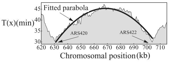
Replication time curves [16] for S. cerevisiae chromosome IV (620–715 kb) with a fitted parabola

X. DISCUSSION AND CONCLUSIONS

In this paper we studied the properties of a mathematical model of chromosome replication that describes genome duplication dynamics in eukaryotic cells. In the first part of the study, we formulated a general model for replication, which takes into account the fact that origins activate stochastically, and also accounts for the possibility that origins in individual cells may not activate at all, because they may have failed to license. We have derived a probability distribution of replication as a function of position and time, and from this we have found analytical expressions for many quantities of interest such as mean replication time, the average number of active origins, and others.

In the second part of the paper, the dynamics of replication was investigated in detail in an idealized scenario for a chromosome with two origins of replication and the activation probability distribution given by a uniform distribution. Despite being idealized, this simple scenario encapsulates much of the essential behavior found in more complex cases; and although organisms vary enormously in the size, shape, and distribution of genomes, the case of the chromosome with just two origins is of biological interest: recently an E. coli mutant with two identical functional replication origins has been constructed [54]. We were able to derive an analytical expression for the mean replication time and to extract hence many important properties of the dynamics of DNA replication. Furthermore, we have proposed a method to determine the width of the activation time probability distribution from experimentally measured population-averaged data. Our results compare favorably with experimental measurements in S. cerevisae.

APPENDIX A. RELATIONSHIP BETWEEN MEAN REPLICATION TIME AND MEAN COPY NUMBER

For a eukaryotic cell with a fixed S phase, the mean replication time can be calculated:

$$T\left(x\right)=\frac{1}{\mathcal{N}}{\int }_{T_1}^{T_2}tP(x,t)\mathit{dt},$$ (A1)

where $\mathcal{N}=1-{\prod }_{i=1}^n{s}_i$, T₁ is the time when replication starts, and T₂ is the time when replication finishes.

The relationship between copy number C(x,t) and fraction replicated m(x,t) is given by Eq. (8). Now, the fraction replicated before time t for cells where replication started at T₁ is given by

$$m(x,t)=\frac{1}{\mathcal{N}}{\int }_{T_1}^{t}P(x,\tau )d\tau .$$ (A2)

The time average of the function m(x,t) is

$$\begin{array}{cc}\hfill \stackrel{‒}{m}\left(x\right)& =\frac{1}{\mathcal{N}}\frac{1}{T_2-T_1}{\int }_{T_1}^{T_2}\mathit{dt}{\int }_{T_1}^{t}P(x,\tau )d\tau \hfill \\ \hfill & =\frac{1}{\mathcal{N}}\frac{1}{T_2-T_1}{\int }_{T_1}^{T_2}d\tau {\int }_{\tau }^{T_2}P(x,\tau )\mathit{dt}\hfill \\ \hfill & =\frac{1}{\mathcal{N}}\frac{1}{T_2-T_1}{\int }_{T_1}^{T_2}P(x,\tau )d\tau {\int }_{\tau }^{T_2}\mathit{dt}\hfill \\ \hfill & =\frac{1}{\mathcal{N}}\frac{1}{T_2-T_1}{\int }_{T_1}^{T_2}P(x,\tau )(T_2-\tau )d\tau \hfill \\ \hfill & =\frac{1}{\mathcal{N}}\frac{1}{T_2-T_1}\left({\int }_{T_1}^{T_2}P(x,\tau )T_{2}d\tau -{\int }_{T_1}^{T_2}\tau P(x,\tau )d\tau \right)\hfill \\ \hfill & =\frac{1}{\mathcal{N}}\frac{1}{T_2-T_1}\left(T_2{\int }_{T_1}^{T_2}P(x,\tau )d\tau -{\int }_{T_2}^{T_1}tP(x,t)\mathit{dt}\right).\hfill \end{array}$$

Taking into account Eq. (A1) and the fact that the first integral in the parentheses equals $1-{\prod }_{i=1}^n{s}_i=\mathcal{N}$, we get

$$\stackrel{‒}{m}\left(x\right)=\frac{T_2-T\left(x\right)}{T_2-T_1}$$ (A3)

and

$$\stackrel{‒}{C}\left(x\right)=\frac{T_2-T\left(x\right)}{T_2-T_1}+1.$$ (A4)

APPENDIX B. REGIMES FOR Δt₁ ≠ Δt₂

Some of the regimes for the case Δt₁ ≠ Δt₂ are shown in Fig. 6(b). Only in this case can the states E and F (Fig. 5) be observed. Also, regimes R₂, R₃, and R₅ have either state E occurring between positions $x=\frac{1}{4}[2D+v(2\tau -\Delta t_1+\Delta t_2\left)\right]$ and $x=\frac{1}{4}[2D+v(2\tau +\Delta t_1-\Delta t_2\left)\right]$ for $\Delta t_1>\Delta t_2$, or state F between positions $x=\frac{1}{4}[2D+v(2\tau +\Delta t_1-\Delta t_2\left)\right]$ and $x=\frac{1}{4}[2D+v(2\tau -\Delta t_1+\Delta t_2\left)\right]$ for Δt₁ < Δt₂. If Δt₁ → Δt₂, the length of this interval decreases until states E and F disappear and position $x=\frac{1}{2}(D+v\tau )$ then separates states C and D.

For regime R₆, state A occurs up to position $x=\frac{1}{4}[2D+v(2\tau -\Delta t_1-\Delta t_2\left)\right]$; then it changes to state C. At position $x=\frac{1}{4}[2D+v(2\tau -\Delta t_1+\Delta t_2\left)\right]$, state C changes to the state E. In a similar way, for regime R₇ state A also occurs up to position $x=\frac{1}{4}[2D+v(2\tau -\Delta t_1-\Delta t_2\left)\right]$; and then it changes to state C. At position $x=\frac{1}{4}[2D+v(2\tau -\Delta t_1+\Delta t_2\left)\right]$, state C changes to the state F.

Other types of regime characteristic for the case Δt₁ ≠ Δt₂ are regime R₈ (Δt₁ ≫ Δt₂), where only state E is possible; and regime R₉ (Δt₂ ≫ Δt₁), where only state F occurs.

For a fixed value of $\Delta t_1\ll \frac{D}{v}$ the regime dynamics as Δt₂ changes are shown in the upper panels of Figs. 6(c) and 6(d). The transitions in the dynamics are given in the table below:

$\tau <\frac{D}{v}$		$\tau <\frac{D}{v}$
Change	Δt1	Change	Δt1
R2 → R3	$2\left(\frac{D}{v}-\tau -\frac{\Delta t_2}{2}\right)$	R1 → R4	$2\left(\tau -\frac{D}{v}-\frac{\Delta t_2}{2}\right)$
R3 → R5	$2\left(\frac{D}{v}-\tau +\frac{\Delta t_2}{2}\right)$	R4 → R6	$2\left(\tau -\frac{D}{v}+\frac{\Delta t_2}{2}\right)$
R5 → R8	$2\left(\tau +\frac{D}{v}+\frac{\Delta t_2}{2}\right)$	R6 → R8	$2\left(\frac{D}{v}+\tau +\frac{\Delta t_2}{2}\right)$

For a fixed value of $\Delta t_2\ll \frac{D}{v}$ the regime dynamics for variable Δt₁ is shown in the lower panels of Figs. 6(c) and 6(d). The transitions are

$\tau <\frac{D}{v}$		$\tau <\frac{D}{v}$
Change	Δt2	Change	Δt2
R2 → R3	$2\left(\frac{D}{v}-\tau -\frac{\Delta t_1}{2}\right)$	R1 → R4	$2\left(\tau -\frac{D}{v}-\frac{\Delta t_1}{2}\right)$
R3 → R5	$2\left(\frac{D}{v}-\tau +\frac{\Delta t_1}{2}\right)$	R4 → R7	$2\left(\tau -\frac{D}{v}+\frac{\Delta t_1}{2}\right)$
R5 → R9	$2\left(\frac{D}{v}+\tau +\frac{\Delta t_1}{2}\right)$	R7 → R9	$2\left(\frac{D}{v}+\tau +\frac{\Delta t_1}{2}\right)$

In the extreme case where $\tau >\frac{D}{v}+\frac{\Delta t_1}{2}+\frac{\Delta t_2}{2}$ the only possible regime is R₁.

APPENDIX C. PROPORTION OF LEFT MOVING FORKS IN REGIME R₂

This is given by

$$n_{\text{left}}\left(x\right)=\{\begin{array}{c}1\text{if}x<0;\hfill \\ \frac{q_2-q_1{q}_2}{q_1+q_2-q_1{q}_2}\text{if}x\in [0;\frac{D+v(\tau -\Delta t)}{2});\hfill \\ -\frac{q_2\{D^2{q}_1-\Delta t^2(-2+q_1)v^2-2{\mathit{Dq}}_1(\Delta \mathit{tv}+2x-v\tau )-2\Delta {\mathit{tq}}_{1}v(-2x+v\tau )+q_1{(-2x+v\tau )}^2\}}{2\Delta t^2\left\{q_1\right(q_2-1)-q_2\}{v}^2}\text{if}x\in [\frac{D+v(\tau -\Delta t)}{2};\frac{D+v\tau }{2});\hfill \\ \frac{q_2\{D^2{q}_1+\Delta t^2(-2+q_1)v^2+2\Delta {\mathit{tq}}_{1}v(-2x+v\tau )+q_1{(-2x+v\tau )}^2+2{\mathit{Dq}}_1(-2x+v\tau +v\Delta t\left)\right\}}{2\Delta t^2\left\{q_1\right(q_2-1)-q_2\}{v}^2}\text{if}x\in [\frac{D+v\tau }{2};\frac{D+v(\tau +\Delta t)}{2});\hfill \\ \frac{q_2}{q_1+q_2-q_1{q}_2}\text{if}x\in [\frac{D+v(\tau +\Delta t)}{2)};D);\hfill \\ 0\text{if}x\ge D.\hfill \end{array}\phantom{\}}$$ (C1)

APPENDIX D. PROBABILITY OF THE FORK TERMINATION POSITION DISTRIBUTION

This is given by

$$P_{\mathrm{ft}}\left(x\right)=\{\begin{array}{c}0\text{if}\tau >\frac{2D+v(\Delta t_1+\Delta t_2)}{2v};\hfill \\ 0\text{if}x<0;\hfill \\ 0\text{if}x>D;\hfill \\ \frac{q_1{q}_2[4x-2D+v(-2\tau +\Delta t_1+\Delta t_2\left)\right]}{2\Delta t_1\Delta t_{2}v(1-s_1{s}_2)}\text{if}x\in [\frac{2D+v(2\tau -\Delta t_1-\Delta t_2)}{4};\frac{D+v\tau }{2}];\hfill \\ \frac{q_1{q}_2[4x+2D+v(2\tau +\Delta t_1+\Delta t_2\left)\right]}{2\Delta t_1\Delta t_{2}v(1-s_1{s}_2)}\text{if}x\in [\frac{D+v\tau }{2};\frac{2D+v(2\tau +\Delta t_1+\Delta t_2)}{4}].\hfill \\ 0\text{otherwise}.\hfill \end{array}\phantom{\}}$$ (D1)

APPENDIX E. SENSITIVITY ANALYSIS OF AN EXPRESSION FOR THE SECOND DERIVATIVE OF THE MEAN REPLICATION TIME

We rewrite Eq. (29) as $G=\frac{A}{\mathsf{g}}$, where $A=\frac{4q_1{q}_2\sqrt{1-\mid 1∕q_1-1∕q_2\mid }}{v^2(1-s_1{s}_2)}$, and g = Δt. Then the change in the value of G with respect to differences in the parameter g is

$$\mid \Delta G\mid =A\left(\frac{1}{\mathsf{g}}-\frac{1}{\mathsf{g}+\Delta \mathsf{g}}\right)=A\frac{\Delta \mathsf{g}}{\mathsf{g}(\mathsf{g}+\Delta \mathsf{g})}$$

For the parameter g in the range (7,18) min [14], a difference of 2 min results in a difference of up to 2.5% in $\frac{\Delta G}{A}$.

Normalization errors and noisy data result in errors in the calculated mean replication time [T(x)]. We have used a simple Monte Carlo simulation technique to roughly estimate how the Δt predicted from formula (29) is affected by errors in the replication time profile T(x). For this simulation we added Gaussian-distributed noise of mean 0 and standard deviation 5 min to each simulated replication profile of a two-origin chromosome, thus mimicking the effects of experimental error (we expect 5 min to be a reasonable estimate of the error for the experiments we use). We then numerically calculate the second derivative of a fitted parabola through the resulting mean replication time curve, and use formula (29) to calculate the “predicted” Δt*, which we can compare with the actual value Δt used to generate T(x) in the first place. We then repeat this procedure 100 times, generating a distribution of Δt*’s, and we do this for a few values of Δt to see how the error affects origins with different variabilities in activation time.

Errors in the estimation of Δt are greatest for origins with low variation in the activation time, as is to be expected. For origins with Δt ≈ 10 min, which is the value we estimated in the example discussed in the paper, the error is around 10%, which shows that formula (29) is quite robust to experimental errors.

References

- [1].Smith J, Martin L. Proc. Natl. Acad. Sci. USA. 1973;70:1263. doi: 10.1073/pnas.70.4.1263. [DOI] [PMC free article] [PubMed] [Google Scholar]
- [2].Blow JJ, Gillespie PJ. Nat. Rev. Cancer. 2008;8:799. doi: 10.1038/nrc2500. [DOI] [PMC free article] [PubMed] [Google Scholar]
- [3].Smith Z, Higgs D. Hum. Mol. Genet. 1999;8:1373. doi: 10.1093/hmg/8.8.1373. [DOI] [PubMed] [Google Scholar]
- [4].de Moura APS, Retkute R, Hawkins M, Nieduszynski CA. Nucleic Acids Res. 2010;38:5623. doi: 10.1093/nar/gkq343. [DOI] [PMC free article] [PubMed] [Google Scholar]
- [5].Retkute R, Nieduszynski CA, de Moura A. Phys. Rev. Lett. 2011;107:068103. doi: 10.1103/PhysRevLett.107.068103. [DOI] [PMC free article] [PubMed] [Google Scholar]
- [6].Hyrien O, Goldar A. Chromosome Res. 2010;18:147. doi: 10.1007/s10577-009-9092-4. [DOI] [PubMed] [Google Scholar]
- [7].Jun S, Zhang H, Bechhoefer J. Phys. Rev. E. 2005;71:011908. doi: 10.1103/PhysRevE.71.011908. [DOI] [PubMed] [Google Scholar]
- [8].Lygeros J, Koutroumpas K, Dimopoulos S, Legouras I, Kouretas P, Heichinger C, Nurse P, Lygerou Z. Proc. Natl. Acad. Sci. USA. 2008;106:9535. doi: 10.1073/pnas.0805549105. [DOI] [PMC free article] [PubMed] [Google Scholar]
- [9].Spiesser T, Klipp E, Barberis M. Mol. Genet. Genom. 2009;282:25. doi: 10.1007/s00438-009-0443-9. [DOI] [PMC free article] [PubMed] [Google Scholar]
- [10].Sekedat MD, Fenyö D, Rogers RS, Tackett AJ, Aitchison JD, Chait BT. Mol. Syst. Biol. 2010;6:353. doi: 10.1038/msb.2010.8. [DOI] [PMC free article] [PubMed] [Google Scholar]
- [11].Hyrien O, Goldar A. Chromosome Res. 2009;18:147. doi: 10.1007/s10577-009-9092-4. [DOI] [PubMed] [Google Scholar]
- [12].Koutroumpas K, Lygeros J. Automatica. 2011;47:1156. [Google Scholar]
- [13].Luo H, Li J, Eshaghi M, Liu J, Karuturi RKM. BMC Bioinf. 2010;11:297. doi: 10.1186/1471-2105-11-247. [DOI] [PMC free article] [PubMed] [Google Scholar]
- [14].Yang SC-H, Rhind N, Bechhoefer J. Mol. Syst. Biol. 2010;6:404. doi: 10.1038/msb.2010.61. [DOI] [PMC free article] [PubMed] [Google Scholar]
- [15].Baker A, Audit B, Chen C-L, Moindrot B, Leleu A, Guilbaud G, Rappailles A, Vaillant C, Goldar A, Mongelard F, d’Aubenton Carafa Y, Hyrien O, Thermes C, Arneodo A. PLoS Comput. Biol. 2012;8:e1002443. doi: 10.1371/journal.pcbi.1002443. [DOI] [PMC free article] [PubMed] [Google Scholar]
- [16].Raghuraman MK, Winzeler EA, Collingwood D, Hunt S, Wodicka L, Conway A, Lockhart DJ, Davis RW, Brewer BJ, Fangman WL. Science. 2001;294:115. doi: 10.1126/science.294.5540.115. [DOI] [PubMed] [Google Scholar]
- [17].Tuduri S, Tourriere H, Pasero P. Chromosome Res. 2010;18:91. doi: 10.1007/s10577-009-9098-y. [DOI] [PubMed] [Google Scholar]
- [18].Kitamura E, Blow JJ, Tanaka TU. Cell. 2006;125:1308. doi: 10.1016/j.cell.2006.04.041. [DOI] [PMC free article] [PubMed] [Google Scholar]
- [19].Friedman KL, Brewer BJ, Fangman WL. Genes Cells. 1997;2:667. doi: 10.1046/j.1365-2443.1997.1520350.x. [DOI] [PubMed] [Google Scholar]
- [20].Rhind N, Yang SC-H, Bechhoefer J. Chromosome Res. 2010;18:35. doi: 10.1007/s10577-009-9093-3. [DOI] [PMC free article] [PubMed] [Google Scholar]
- [21].Shor E, Warren CL, Tietjen J, Hou Z, Müller U, Alborelli I, Gohard FH, Yemm AI, Borisov L, Broach JR, Weinreich M, Nieduszynski CA, Ansari AZ, Fox CA. PLoS Genet. 2009;5:e1000755. doi: 10.1371/journal.pgen.1000755. [DOI] [PMC free article] [PubMed] [Google Scholar]
- [22].Kolmogorov A. Izv. Akad. Nauk. SSSR. 1937;1:335. [Google Scholar]
- [23].Andrienko YA, Brilliantov NV, Krapivsky PL. Phys. Rev. A. 1992;45:2263. doi: 10.1103/physreva.45.2263. [DOI] [PubMed] [Google Scholar]
- [24].Al-Mahboob A, Fujikawa Y, Sadowski JT, Hashizume T, Sakurai T. Phys. Rev. B. 2010;82:235421. [Google Scholar]
- [25].Yabuki N, Terashima H, Kitada K. Genes Cells. 2002;7:781. doi: 10.1046/j.1365-2443.2002.00559.x. [DOI] [PubMed] [Google Scholar]
- [26].Gilbert DM. Nat. Rev. Genet. 2010;11:673. doi: 10.1038/nrg2830. [DOI] [PMC free article] [PubMed] [Google Scholar]
- [27].Müller CA, Nieduszynski CA. Genome Res. 2012 doi: 10.1101/gr.139477.112. doi: 10.1101/gr.139477.112 (2012) [DOI] [PMC free article] [PubMed] [Google Scholar]
- [28].Woodfine K, Fiegler H, Beare D, Collins J, McCann O, Young B, Debernardi S, Mott R, Dunham I, Carter N. Hum. Mol. Genet. 2004;13:191. doi: 10.1093/hmg/ddh016. [DOI] [PubMed] [Google Scholar]
- [29].Schubeler D, Scalzo D, Kooperberg C, van Steensel B, Delrow J, Groudine M. Nat. Genet. 2002;32:438. doi: 10.1038/ng1005. [DOI] [PubMed] [Google Scholar]
- [30].Ryba T, Battaglia D, Pope BD, Hiratani I, Gilbert DM. Nat. Protoc. 2011;6:870. doi: 10.1038/nprot.2011.328. [DOI] [PMC free article] [PubMed] [Google Scholar]
- [31].Yaffe E, Farkash-Amar S, Polten A, Yakhini Z, Tanay A, Simon I. PloS Genet. 2010;6:e1001011. doi: 10.1371/journal.pgen.1001011. [DOI] [PMC free article] [PubMed] [Google Scholar]
- [32].Koren A, Soifer I, Barkai N. Genome Res. 2010;20:781. doi: 10.1101/gr.102764.109. [DOI] [PMC free article] [PubMed] [Google Scholar]
- [33].Koren A, Tsai H-J, Tirosh I, Burrack LS, Barkai N, Berman J. PloS Genet. 2010;6:e1001068. doi: 10.1371/journal.pgen.1001068. [DOI] [PMC free article] [PubMed] [Google Scholar]
- [34].Ma M, Hyrien O, Goldar A. Nucleic Acids Res. 2012;40:2010. doi: 10.1093/nar/gkr982. [DOI] [PMC free article] [PubMed] [Google Scholar]
- [35].Goldar A, Marsolier-Kergoat M-C, Hyrien O. PloS One. 2009;4:1. doi: 10.1371/journal.pone.0005899. [DOI] [PMC free article] [PubMed] [Google Scholar]
- [36].Raghuraman MK, Brewer BJ. Chromosome Res. 2010;18:19. doi: 10.1007/s10577-009-9099-x. [DOI] [PMC free article] [PubMed] [Google Scholar]
- [37].Anglana M, Apiou F, Bensimon A, Debatisse M. Cell. 2003;114:385. doi: 10.1016/s0092-8674(03)00569-5. [DOI] [PubMed] [Google Scholar]
- [38].Bechhoefer J, Marshall B. Phys. Rev. Lett. 2007;98:098105. doi: 10.1103/PhysRevLett.98.098105. [DOI] [PubMed] [Google Scholar]
- [39].Fachinetti D, Bermejo R, Cocito A, Minardi S, Katou Y, Kanoh Y, Shirahige K, Azvolinsky A, Zakian VA, Foiani M. Mol. Cell. 2010;39:595. doi: 10.1016/j.molcel.2010.07.024. [DOI] [PMC free article] [PubMed] [Google Scholar]
- [40].Blow JJ, Ge XQ, Jackson DA. Trends Biochem. Sci. 2011;36:405. doi: 10.1016/j.tibs.2011.05.002. [DOI] [PMC free article] [PubMed] [Google Scholar]
- [41].Letessier A, Millot GA, Koundrioukoff S, Lachages A-M, Vogt N, Hansen RS, Malfoy B, Brison O, Debatisse M. Nature (London) 2011;470:120. doi: 10.1038/nature09745. [DOI] [PubMed] [Google Scholar]
- [42].Patel P, Arcangioli B, Baker S, Bensimon A, Rhind N. Mol. Biol. Cell. 2006;17:308. doi: 10.1091/mbc.E05-07-0657. [DOI] [PMC free article] [PubMed] [Google Scholar]
- [43].Blow J, Dutta A. Nat. Rev. Mol. Cell Biol. 2005;6:476. doi: 10.1038/nrm1663. [DOI] [PMC free article] [PubMed] [Google Scholar]
- [44].Conti C, Sacca B, Herrick J, Lalou C, Pommier Y, Bensimon A. Mol. Biol. Cell. 2007;18:3059. doi: 10.1091/mbc.E06-08-0689. [DOI] [PMC free article] [PubMed] [Google Scholar]
- [45].Tuduri S, Tourrière H, Pasero P. Chromosome Res. 2010;18:91. doi: 10.1007/s10577-009-9098-y. [DOI] [PubMed] [Google Scholar]
- [46].Rivin C, Fangman W. J. Cell Biol. 1980;85:108. doi: 10.1083/jcb.85.1.108. [DOI] [PMC free article] [PubMed] [Google Scholar]
- [47].Smith DJ, Whitehouse I. Nature (London) 2012;483:434. doi: 10.1038/nature10895. [DOI] [PMC free article] [PubMed] [Google Scholar]
- [48].Parameter values used were q1 = 0.96, q2 = 0.88, τ = 4, Δt = 10, and ν = 1.6 kb/min, estimated as described in [4].
- [49].Lundgren M, Andersson A, Chen L, Nilsson P, Bernander R. Proc. Natl. Acad. Sci. USA. 2004;101:7046. doi: 10.1073/pnas.0400656101. [DOI] [PMC free article] [PubMed] [Google Scholar]
- [50].Norais C, Hawkins M, Hartman AL, Eisen JA, Myllykallio H, Allers T. PloS Genet. 2007;3:729. doi: 10.1371/journal.pgen.0030077. [DOI] [PMC free article] [PubMed] [Google Scholar]
- [51].Duggin IG, Dubarry N, Bell SD. EMBO J. 2011;30:145. doi: 10.1038/emboj.2010.301. [DOI] [PMC free article] [PubMed] [Google Scholar]
- [52].Siow CC, Nieduszynska SR, Müller CA, Nieduszynski CA. Nucleic Acids Res. 2011;40:D682. doi: 10.1093/nar/gkr1091. [DOI] [PMC free article] [PubMed] [Google Scholar]
- [53].Parameter values used were q1 = 0.68, q2 = 0.73, and ν = 1.6 kb/min, estimated in [4].
- [54].Wang X, Lesterlin C, Reyes-Lamothe R, Ball G, Sherratt DJ. Proc. Natl. Acad. Sci. USA. 2011;108:E243. doi: 10.1073/pnas.1100874108. [DOI] [PMC free article] [PubMed] [Google Scholar]