Recording and Analyzing IFT in Chlamydomonas Flagella

Abstract

The transport of materials to and from the cell body and tips of eukaryotic flagella and cilia is carried out by a process called intraflagellar transport, or IFT. This process is essential for the assembly and maintenance of cilia and flagella: in the absence of IFT, cilia cannot assemble and, if IFT is arrested in ciliated cells, the cilia disassemble. The major IFT complex proteins and the major motor proteins, kinesin-2 and osm-3 (which transport particles from the cell body to ciliary tips) and cytoplasmic dynein 1b (which transports particles from ciliary tips to the cell body) have been identified. However, we have little understanding of the structure of the IFT particles, the cargo that these particles carry, how cargo is loaded and unloaded from the particles, or how the motor proteins are regulated. The focus of this chapter is to provide methods to observe and quantify the movements of IFT particles in Chlamydomonas flagella. IFT movements can be visualized in paralyzed or partially arrested flagella using either differential interference contrast (IFT) microscopy or, in cells with fluorescently tagged IFT components, with fluorescence microscopy. Methods for recording IFT movements and analyzing movements using kymograms are described.

I. Introduction

Intraflagellar transport (IFT) first was observed using a specialized differential interference contrast (DIC) microscope and recording system (Kozminski, 1995; Kozminski et al., 1993). The elegant movies of particle movement within flagella and use of the ts-mutant fla10 to identify the anterograde motor for IFT (Kozminski et al., 1995) led to a new area in studies of cilia and flagella and the discovery of ciliary defects associated with a number of human diseases, or ciliopathies (Badano et al., 2006; Marshall, 2008).

Analysis of the rapid bidirectional movement of IFT particles in 0.2-μm diameter flagella was made possible by the development of kymograms that displayed particle positions along the flagellum as a function of time (Iomini et al., 2001; Piperno et al., 1998). Although these techniques were major advances in the field, they required equipment and computer programs that were not generally available, so their application was limited. Recent improvements in microscope optics, recording equipment, and computer programs have made it possible for most investigators to visualize IFT at modest cost (Dentler, 2005; Mueller et al., 2005). These techniques permit the analysis of anterograde and retrograde IFT as well as the movement of particles along flagellar surfaces using high-resolution DIC (Fig. 1). With the development of green fluorescent protein (GFP)-tagged IFT components (Mueller et al., 2005; Snow et al., 2004) IFT can be observed using wide-field fluorescence microscopy (Fig. 2).

Fig. 1.

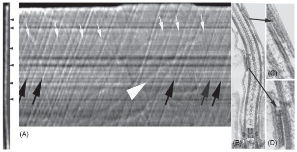
IFT particle movement analyzed using kymographs. (A) A flagellum with IFT particles (arrowheads) is shown to the left of “A” and a kymograph showing the movement of these particles is at the right of the flagellum. Anterograde particles move toward the flagellar tip (black arrows) and smaller retrograde particles move toward the base of the flagellum (white arrows). The white arrowhead points to a larger and slowly moving particle, likely moving along the flagellar surface. (B) Thin section of Chlamydomonas flagella showing IFT particles with higher magnification images shown in (C) and (D). It is not known if these are anterograde or retrograde particles.

Fig. 2.

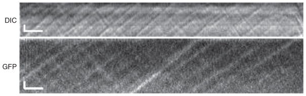
Comparison of IFT by DIC and wide-field fluorescence microscopy recorded with a digital camera. The vertical bar is 1 μm and the horizontal bar is 1 s.

The purpose of this chapter is to provide methods that can be used to observe, record, and measure IFT using commercially available equipment. It will be focused on observations of IFT in Chlamydomonas flagella, because the long flagella are ideal specimens to observe IFT. IFT can be observed using DIC and, with GFP-tagged IFT components, by fluorescence microscopy. The analytical methods described here also are useful for analyzing fluorescently labeled flagella, regardless of the organism from which images were captured.

II. Methods

The most important decision is to choose cells with long and relatively immobile flagella. In our hands, pf18, a Chlamydomonas mutant that lacks central microtubules and has fairly straight and rigid flagella, is the easiest strain with which to observe IFT. The flagella attach to coverslips and IFT can be observed throughout the flagellum from the base, where flagella exit the cell wall, to the distal tips. Other paralyzed flagellar mutants to consider include pf16, which has an unstable C1 microtubule, and pf1, which lacks spoke heads (Kozminski, 1995). For many experiments, motile cells need to be examined, and so methods to immobilize these cells also are described in this chapter.

A. Slide Preparation

Slides and coverslips must be clean for optimal imaging. They can be cleaned by soaking in hot water and detergent followed by extensive washing with deionized water and air or oven drying. Alternatively, they can be cleaned by an overnight soak in 6 N HCl followed by extensive washing in deionized water, rinsing in 95% EtOH, and air drying (Kozminski, 1995).

For DIC, thin (#0) coverslips can be used as a slide and coverslip. An aluminum slide is cut from a 1-mm-thick aluminum sheet and an opening, ~7.5 cm ×3 cm, is cut out for the coverslip. A clean 24-mm ×60-mm No 0 coverslip (Gold Seal #3223) is attached to the bar by double stick tape and two small (~2 mm ×20 mm) Parafilm spacers are placed on the large coverslip before mounting cells attached to a smaller coverslip (below) to avoid crushing and deflagellating cells.

DIC and fluorescence microscopy also can be carried out using standard cleaned glass slides and #1 or 1.5 coverslips. If cells are mounted in agar (below), the spacers are not needed.

B. Specimen Preparation

Observation of IFT in paralyzed mutants is relatively straightforward and primarily requires patience. Observation of IFT in nonparalyzed cells requires mechanical or chemical methods to paralyze flagella. In each of these methods, cells are applied to coverslips and allowed to sit for 2–5 min. This promotes attachment of flagella to the coverslips, which is essential for observing IFT.

Attachment of flagella to coverslips is facilitated by coating coverslips with 0.01–1 mg/ml poly-L-lysine (Sigma Corporation, St. Louis, MO P1274). Higher concentrations of polylysine will induce flagella to curl and to detach from cells (Blood-good, 1981). Polylysine is applied to clean cover glasses and allowed to sit for 5 min to overnight. Then rinse coverslips with water and air dry. Apply cells to the coverslips, allow cells to attach, and then invert the coverslips over the larger coverslip or slide with Parafilm spacers. Withdraw as much of the medium as possible using filter paper and seal the slides with VALAP.

Agarose can be used to mechanically immobilize motile cells. Kozminski (1995) formed a small agar chamber beneath the coverslip and placed cells in the chamber. We have had more success using 1–2% low EEO agarose (Fisher Scientific BP160) dissolved in culture medium and maintained at ~30°C. Apply the cells to a coverslip and allow them to attach for 2–5 min. Remove most of the media, add 8–10 μl of the agarose solution to the cells, invert over a slide, and seal with VALAP.

VALAP is made by adding equal weights of Vaseline, lanolin, and paraffin to a beaker and heating to melt the mixture. VALAP can be stored indefinitely at room temperature. For use, melt VALAP and apply to the slide with a glass Pasteur pipette. Flatten the bead of VALAP with a warm spatula to minimize the possibility of contaminating the objective lens.

Motile flagella can be paralyzed by adding 20 mM LiCl to the mounting medium. Although LiCl induces flagellar growth (Nakamura et al., 1987; Periz et al., 2007), little growth occurs in the time during which IFT is recorded and 20 mM LiCl does not induce changes in the rate or frequency of anterograde or retrograde IFT (Dentler, 2005). Used cautiously, addition of 10–20 mM LiCl can facilitate recording IFT in motile flagella.

C. Microscopy

1. Differential Interference Contrast

IFT was discovered using DIC microscopy and high-resolution objective and condenser lenses. Our best images are obtained using infinity-corrected optics and a Zeiss (Carl Zeiss, Thornwood, NY, USA) Axioplan 2ie upright microscope. Most flagella remain attached to the cover glass in the upright microscope but it is possible that an inverted microscope may maintain better attachment of flagella and better imaging.

Full and even illumination of the back focal plane of the condenser lens is essential for high-resolution imaging. With fixed tube length optics, a mercury or xenon lamp and a fiber-optic scrambler was essential to obtain sufficient illumination to produce high-quality images (Kozminski, 1995; Piperno et al., 1998). In our experience, this intense light damages the cells even after short periods of illumination. Light transmission is greatly improved with newer infinity-corrected optics and we currently use a standard halogen lamp built into the microscope base. Together with a UV- and IR-absorbing filter and a green interference filter, cells can be observed for at least 3 h without any visible damage.

High-resolution DIC requires objective and condenser lenses with numerical apertures of 1.4 or greater. Immersion oil must be used between the slide and condenser lens and between the coverslip and objective lens. The microscope must be properly aligned to produce full Koehler illumination.

To record IFT the long axis of the flagellum should fill the camera field as much as possible. This requires 100× NA1.4 planapochromat (for DIC) or 100× NA 1.3 plan fluar (for fluorescence) objective lenses. The image should be projected on the camera face using a 1.6× Bertrand lens (Optovar), and an 8× eyepiece or a 1.2× TV tube magnifier.

a. Specimen Orientation

Proper specimen orientation is essential. Normally, flagella are best observed when their long axis is perpendicular to the shear axis. For IFT, flagella must be positioned so that their long axis is parallel to the shear axis. The IFT particles then will move perpendicular to the shear axis and be shadowed. When properly oriented, the flagellum may be nearly invisible when observed through the microscope eyepieces but the increased contrast provided by the video camera and computer will make the flagellum and IFT visible on a monitor. While flagella in the proper orientation to the shear axis can be found by randomly scanning the slide, it is helpful to have a properly aligned rotating stage, so that the flagellum can be rotated to lie in the proper shear axis. For our Axioplan 2ie microscope, if a cell body is in the center of the field, the flagellum should point to ~10 o’clock for optimal orientation.

Flagella are most easily selected by scanning by eye. To observe flagella, close the condenser aperture diaphragm and scan the field. When the specimen to be recorded is found, open the diaphragm to fill the back focal plane for maximum resolution, and view the flagella on the monitor.

2. Fluorescence Microscopy

IFT also can be observed in tissues or in protozoan flagella if IFT particles contain fluorescently tagged molecules (Mueller et al., 2005; Snow et al., 2004). Some microscopy facilities may have better equipment for fluorescence microscopy than they do for DIC, so capturing IFT using fluorescence microscopy should be considered.

The major disadvantages of fluorescence microscopy include the requirement for a fluorescently tagged IFT particle or motor protein subunit and problems associated with photobleaching and phototoxicity. The primary requirements for microscope optics and specimen preparation are the same as described for DIC (above).

To minimize photobleaching, first find and orient flagella with observable IFT using DIC. Then switch to fluorescent illumination and record a series of images. Photo-toxicity can be a major problem and high levels of UV light can result in GFP-tagged IFT particles slowing down after ~30 s. To minimize photobleaching and phototoxic effects, we use an X-cite light (CanadaExfo Photonics Solutions, Mississauga, Ontario, Canada) at an intensity of 75% or less to observe movements of GFP-tagged kinesin-associated protein subunits (Mueller et al., 2005). Using these conditions, IFT can be observed and recorded for up to 1 min. Others have successfully used laser illumination systems to observe movements of GFP-tagged IFT particles (Qin et al., 2007). Use of monochromatic light sources also may reduce phototoxicity. Preliminary reports on the use of TIRF microscopy to study IFT are promising (see Chapter 9 by Engel et al., this volume).

Are the same particles observed using DIC and fluorescence microscopy? Comparisons of IFT recorded by fluorescence and DIC microscopy (Fig. 2) indicate that it is likely that the same anterograde particles are observed by both methods. However, the smaller retrograde IFT particles (Dentler, 2005; Iomini et al., 2001; Mueller et al., 2005) are more difficult to resolve using fluorescence microscopy, so many movies and kymographs must be examined to have a sufficient number of particle tracks to confidently assess the retrograde IFT rates using fluorescence microscopy.

D. Recording IFT

1. Cameras

A variety of cameras are available for microscopy, and each laboratory will likely have their own specific equipment. It is helpful to mount the camera on the microscope so that the camera can be rotated to orient the flagellum vertically on the screen. This reduces the size of the image to be captured, and reduces the memory required for image capture, and allows one to focus on IFT within the flagellum.

Our most reliable camera for DIC observations is a Nuvicon Video Camera (NC-70, DAGE-MTI, Michigan City, IN, USA). The camera is sufficiently sensitive to record IFT using halogen lamps (above) and adjustments are adequate to produce high-contrast images. Additional image enhancement can be done by sending the video signal through an Avio Image Σ processor, but to our knowledge, this equipment no longer is available. The Nuvicon camera must be used with a frame grabber card such as the Scion FG-7 (www.scioncorp.com), which can be used with Macintosh (OS10) and PC computers and Windows (Microsoft Corporation, Redmond, WA, USA). Digital cameras also can be used. We have had limited experience using an Orca ER (Hammamatsu Phototonics, Hammamatsu City, Japan) and find that it produces excellent images, depending on the capture software and computer buffering capacity.

For fluorescence microscopy, a highly sensitive digital camera must be used along with the appropriate light source. The camera must be sufficiently sensitive to detect a fluorescent signal in a flagellum and be fast enough to record particles moving at IFT rates. We have had the best experience with a Rolera MGi EMCCD camera, Q-Imaging, Surry, British Columbia, Canada (www.qimaging.com). Standard GFP filter sets should be sufficient to image GFP-tagged IFT particles, although a Semrock GFP-3035B filter set (www.Semrock.com) provides significantly brighter GFP images than conventional filters. Be aware that the DIC images taken with digital cameras are not as crisp as those taken with the Nuvicon camera, but this is a trade-off between magnification and light intensity that must be made to collect both DIC and fluorescent images from the same camera.

2. Image capture

Image capture can be carried out with a variety of cameras and programs. Two methods that we use are described below. We also have successfully used Slidebook software (http://www.intelligent-imaging.com/home.php) and a Hamamatsu Orca ER (www.hamamatsu.com) camera to capture images, but, for DIC, find the Nuvicon cameras to work slightly better than the digital cameras.

It is helpful, although not essential, to have a second (live) monitor that can be used to view and focus the live image. The signal from the camera passes through the live monitor and then into the frame grabber in the computer, where the image appears on the computer monitor.

a. Scion Image (Scion Corporation, Frederick, MD, USA)

The least expensive method, in terms of equipment and software, is to use a Nuvicon video camera, Scion frame grabber, and a Macintosh or PC computer. The computer requirements are modest: most of our images were captured with a Macintosh 7600 computer with 512 MB of RAM and a Scion VG5 frame grabber. A more modern computer with additional memory and newer frame-grabber board will allow capture of larger image stacks. The Nuvicon camera and controller are relatively inexpensive and the Image J program is free (http://rsbweb.nih.gov/ij/).

The following steps describe the capture process with the Scion VG5 frame grabber and Scion Image (http://www.scioncorp.com/frames/fr_technical_support.htm). For the newer FG7 frame grabber, software for Windows and Macintosh computers can be downloaded from Scion (http://www.scioncorp.com/frames/fr_technical_support.htm). Install the appropriate plug-ins into Image J before capturing image stacks using Image J.

1. Place the specimen on the microscope stage, focus the specimen, adjust the condenser focus, and open the field and condenser diaphragms to achieve Koehler illumination.

2. Select cells with straight flagella attached to the coverslips. If possible, select cells that are oriented parallel to the DIC shear. Most of the time, flagella will need to be oriented by rotating the microscope stage to orient the flagellum parallel to the DIC shear. In a Zeiss Axioplan, orient the flagella to point to ~10 o’clock, or ~315°.

3. Open Scion Image and select Special>Camera(Live).

4. Optimize image contrast using the camera controller.

5. Adjust image contrast and the DIC slider to obtain the best image on the computer and on the live monitor.

6. Rotate the camera to orient the image of the flagellum so the flagellum is vertical on the monitor.

7. Select a rectangular area to select the flagellum.

8. Set up to capture a movie. Stacks>Make Movie (movies are simply stacks of images).

   1. Select the number of frames to be captured. We usually use 600 frames, depending on the amount of memory available. Record the number of frames and the time of recording for measurements.

   2. Select the frame rate— usually 30 frames/s

9. Press “OK.” The computer will set up a buffer for the frames and will start to collect the images. Some adjustment for focus may need to be made. This is easily done looking at the “live” monitor but can be done viewing the computer image.

10. When frames are captured, save the movie to a file.

b. Metamorph (Molecular Devices, Downington, PA, USA)

The following steps are for Metamorph Version 7.5.6. Some older versions of Metamorph have a bug in the kymograph program that can lead to errors in the estimation of distance and should be used with caution.

1. Open the program and select Acquire>Acquire>Show Live.

2. Select the Center Quad camera area to increase the camera’s frame rate capability.

3. Select and adjust the EM gain in the Special tab in the Acquire window. A good starting range is 5 MHz, at a value around 2000.

4. Select an exposure time so that the camera’s frame rate is 10–30 frames/s. Do not use binning, or the image quality will be too poor for analysis.

5. Set up to capture a movie. Select Acquire>Stream Acquisition. Then, select the number of frames and hit the acquire button to capture the movie.

6. After the movie is acquired, save the movie.

E. IFT analysis

IFT particles rapidly move up and down the flagellum, so it is essential to visually separate anterograde and retrograde particles by preparing kymographs that reveal the location of each particle relative to the time recorded (Iomini et al., 2001). Anterograde particles, moving from base to tip are readily distinguished from retrograde particles, which move from the tip to the flagellar base. The size of the particles can be estimated from the thickness of the path. Kymographs are easily generated using Image J or Metamorph (version 7.5.6)

1. Kymograph Preparation

a. Image J

1. Individual kymographs

1. Open the captured movies (image stack) with Image J and rotate flagellar image stacks so that the flagella is vertical (Image>Rotate>Arbitrarily).

2. Use the rectangle tool to make a rectangular selection of the flagellum, cropping as close as possible to the flagellum.

3. Adjust contrast (Image>adjust>brightness/contrast). Set the maximum and minimum sliders to include the areas in the histogram. Click “Apply” to apply the contrast change to all frames in the image stack.

4. Reslice the image (Image>Stacks>Reslice). Select “Start At”: Left and click the Rotate 90 Degrees box. Then select “OK.” A “Reslice” image will open. This may be relatively faint, so the image can be greatly improved using “Z-project.”

5. Move the slider on the bottom of the Reslice window to select the frames that best show the IFT tracks.

6. With the Reslice window active, select Image>Stacks>Z project. Ignore the warning window and click OK.

7. Select start and stop slices. This can be ignored, if the flagellum is closely cropped, or the slices can be selected by observing the slices that show the best image as the slider in the Reslice window is moved. Select Average Intensity and click OK.

8. A kymogram showing anterograde and retrograde transport will appear in a new window, AVG_Reslice of (file name).

9. Save the kymogram as a tiff file (File>Save As…)

2. Kymograph montage

To analyze IFT, collect as many movies as possible. Some will show better IFT than others. To compare all tracks in various experiments, a montage combining all kymograms from an experiment can be prepared using Photoshop (Adobe Systems, INC, San Jose, CA, USA). Kymograph images are then sharpened and enhanced to visualize the IFT tracks and to allow comparison among different experiments.

1. Open each kymograph, adjust contrast with “levels” (select Auto), and copy the kymograph to a single Photoshop page. When all kymograms are arranged on the page, flatten the image layers (Layer>Flatten) and crop the image.

2. To enhance the images:

   1. Select the entire montage and apply Gaussian Blur (Filter>Blur>Gaussian Blur). Select 0.7 pixels and press OK.

   2. Apply Unsharp Mask (Filter>Sharpen>Unsharp Mask). Select 298%, 2.7 pixels, threshold =1 and press OK. This will provide a good set of kymograms in which IFT tracks are readily visible.

3. Save the final filtered montage as an uncompressed TIFF file for analysis with Image J

b. Metamorph

1. Open the captured movie with Metamorph.

2. Adjust digital contrast to best see IFT (Display>Adjust Digital Contrast).

3. Set up to make the kymograph (Stack>Kymograph).

4. Draw a straight line using the line tool along the length of the flagellum. Change the line width in the Kymograph window to cover the width of the flagellum.

5. Select which frames to make the Kymograph from. All frames can be used if the “All frames” box is checked.

6. Select Create to make the kymograph.

7. Adjust digital contrast on the kymograph so that the IFT tracks are most clearly seen.

8. Save the kymograph as a tiff file (File>Save).

2. Kymograph Analysis

IFT particle rates and frequencies are manually scored by analyzing kymograms with Image J or Metamorph software. For IFT rates, measure the angle of each anterograde (up and to the right) and each retrograde (down and to the right) track using the Image J angle tool or the Metamorph line tool. Save each measurement. Both Image J and Metamorph measurements can be opened in commonly used spreadsheets. Be certain to record the frame rate of the movie by dividing the total number of images (frames) by the recording time. The rate of movement is a function of the tangent of the measured angle of IFT movement and the measured length of the flagellum. The frequency (number of anterograde or retrograde tracks/time) is measured by counting the number of tracks and dividing by the time recorded.

Estimation of IFT particle frequencies with the fluorescent images is somewhat more problematic due to potential bleaching of the signal over the time course of image capture. We typically use only the first 30 s of a recording to estimate particle frequencies.

III. Summary

Recording and analyzing IFT is relatively simple and can be accomplished using commercially available cameras, computers, and software packages. Here we described two different packages but similar results can be obtained with other software. It is critical to have high-resolution optics, microscopes with high light throughput, and, for DIC, properly aligned the optics and flagellar orientation relative to the DIC shear. Of equal importance is patience. Frequently, one will start recording flagella exhibiting beautiful IFT only to find that the cell becomes camera-shy and glides out of the field of view. With patience and experience, however, IFT recordings are easily made.

References

- Badano JL, Mitsuma N, Beales PL, Katsanis N. The ciliopathies: An emerging class of human genetic disorders. Annu Rev Genomics Hum Genet. 2006;7:125–148. doi: 10.1146/annurev.genom.7.080505.115610. [DOI] [PubMed] [Google Scholar]
- Bloodgood RA. Flagella-dependent gliding motility in Chlamydomonas. Protoplasma. 1981;106:183–192. [Google Scholar]
- Dentler WL. Intraflagellar transport (IFT) during assembly and disassembly of Chlamydomonas flagella. J Cell Biol. 2005;170(4):649–659. doi: 10.1083/jcb.200412021. [DOI] [PMC free article] [PubMed] [Google Scholar]
- Iomini C, Babaev-Khaimovm V, Sassaroli M, Piperno G. Protein particles in Chlamydomonas flagella undergo a transport cycle consisting of four phases. J Cell Biol. 2001;153(1):13–24. doi: 10.1083/jcb.153.1.13. [DOI] [PMC free article] [PubMed] [Google Scholar]
- Kozminski KG. High-resolution imaging of flagella. Methods Cell Biol. 1995;47:263–271. doi: 10.1016/s0091-679x(08)60819-5. [DOI] [PubMed] [Google Scholar]
- Kozminski KG, Beech PL, Rosenbaum JL. The Chlamydomonas kinesin-like protein FPA10 is involved in motility associated with the flagellar membrane. J Cell Biol. 1995;131:1517–1527. doi: 10.1083/jcb.131.6.1517. [DOI] [PMC free article] [PubMed] [Google Scholar]
- Kozminski KG, Johnson KA, Forscher P, Rosenbaum JL. A motility in the eukaryotic flagellum unrelated to flagellar beating. Proc Natl Acad Sci USA. 1993;90:5519–5523. doi: 10.1073/pnas.90.12.5519. [DOI] [PMC free article] [PubMed] [Google Scholar]
- Marshall WF. The cell biological basis of ciliary disease. J Cell Biol. 2008;180(1):17–21. doi: 10.1083/jcb.200710085. [DOI] [PMC free article] [PubMed] [Google Scholar]
- Mueller J, Perrone CA, Bower R, Cole DG, Porter ME. The FLA3KAP subunit is required for the localization of kinesin-2 to the site of flagellar assembly and processive anterograde intraflagellar transport. Mol Biol Cell. 2005;16(3):1341–1354. doi: 10.1091/mbc.E04-10-0931. [DOI] [PMC free article] [PubMed] [Google Scholar]
- Nakamura S, Tabino H, Kojima MK. Effect of lithium on flagellar length in Chlamydomonas reinhardtii. Cell Struct Funct. 1987;12:369–374. [Google Scholar]
- Periz G, Dharia D, Miller SH, Keller LR. Flagellar elongation and gene expression in Chlamydomonas reinhardtii. Eukaryot Cell. 2007;6(8):1411–1420. doi: 10.1128/EC.00167-07. [DOI] [PMC free article] [PubMed] [Google Scholar]
- Piperno G, Siuda E, Henderson S, Segil M, Vaananen H, Sassaroli M. Distinct mutants of retrograde intraflagellar transport (IFT) share similar morphological and molecular defects. J Cell Biol. 1998;143(6):1591–1601. doi: 10.1083/jcb.143.6.1591. [DOI] [PMC free article] [PubMed] [Google Scholar]
- Qin H, Wang Z, Diener D, Rosenbaum J. Intraflagellar transport protein 27 is a small G protein involved in cell-cycle control. Curr Biol. 2007;17(3):193–202. doi: 10.1016/j.cub.2006.12.040. [DOI] [PMC free article] [PubMed] [Google Scholar]
- Snow JJ, Ou G, Gunnarson AL, Regina M, Walker S, Zhou HM, Brust-Mascher I, Scholey JM. Two anterograde intraflagellar transport motors cooperate to build sensory cilia on C. elegans neurons. Nat Cell Biol. 2004;6:1109–1113. doi: 10.1038/ncb1186. [DOI] [PubMed] [Google Scholar]