

Abstract
The acquisition time of BOLD contrast functional MRI (fMRI) data with whole-brain coverage typically requires a sampling rate of one volume in 1 3 seconds. Although the volumetric sampling time of a few seconds is adequate for measuring the sluggish hemodynamic response (HDR) to neuronal activation, faster sampling of fMRI might allow for monitoring of rapid physiological fluctuations and detection of subtle neuronal activation timing information embedded in BOLD signals. Previous studies utilizing a highly accelerated volumetric MR inverse imaging (InI) technique have provided a sampling rate of one volume per 100 ms with 5 mm spatial resolution. Here, we propose a novel modification of this technique, the echo-shifted InI, which allows TE to be longer than TR, to measure BOLD fMRI at an even faster sampling rate of one volume per 25 ms with whole-brain coverage. Compared with conventional EPI, echo-shifted InI provided 80-fold speedup with similar spatial resolution and less than 2-fold temporal SNR loss. The capability of echo-shifted InI to detect HDR timing differences was tested empirically. At the group level (n=6), echo-spaced InI was able to detect statistically significant HDR timing differences of as low as 50 ms in visual stimulus presentation. At the level of individual subjects, significant differences in HDR timing were detected for 400 ms stimulus-onset differences. Our results also show that the temporal resolution of 25 ms is necessary for maintaining the temporal detecting capability at this level. With the capabilities of being able to distinguish the timing differences in the millisecond scale, echo-shifted InI could be a useful fMRI tool for obtaining temporal information at a time scale closer to that of neuronal dynamics.
Keywords: echo-shifting, inverse imaging, fMRI, parallel imaging
INTRODUCTION
Volumetric acquisitions of whole-brain functional MRI (fMRI) (Belliveau et al., 1991) using the blood-oxygen-level-dependent (BOLD) contrast (Kwong et al., 1992, Ogawa et al., 1990) typically have a sampling rate of one volume per 1 3 seconds with about 3-mm spatial resolution, and this is used to observe the hemodynamic response (HDR) secondary to neuronal activity (Logothetis et al., 2001). While this sampling rate has been considered sufficient for monitoring the rather sluggish HDR, higher sampling rates might help reveal underlying neuronal dynamics and their behavioral correlates (Menon et al., 1998, Ogawa et al., 2000). High sampling rate on BOLD fMRI could also help monitor and suppress rapid physiological fluctuations in fMRI time series and accordingly to improve the detection sensitivity to brain activity (Lin et al., 2011, Särkkä et al., 2012).
The acquisition time of traditional Fourier-encoded MRI is constrained by the k-space traversal time. Echo-planar imaging (EPI) (Mansfield, 1977) and spiral imaging (Blum et al., 1987) utilize high gradient slew rates and strong high strength MRI gradients to achieve fast k-space traversal. The sampling rate for EPI could also be moderately improved by exploiting the symmetry in the k-space (McGibney et al., 1993). Parallel MRI using the spatial information among different channels of a receiving coil array can also help accelerate the data acquisition, using techniques such as k-space SMASH (Sodickson and Manning, 1997), or GRAPPA (Griswold et al., 2002) methods, or the image domain SENSE (Pruessmann et al., 1999) method. In fMRI, parallel MRI has been successfully combined with the gradient-echo EPI accelerated acquisitions (Preibisch et al., 2003, Schmidt et al., 2005). It has also been demonstrated that incorporating a static image as prior information can further improve the sensitivity of fMRI (Lin et al., 2005).
Other multi-slice-based approaches such as echo-shifted multi-slice EPI (Gibson et al., 2006), Multiplexed-EPI (M-EPI) (Feinberg et al., 2010) and blipped-CAIPI (Setsompop et al., 2012) can acquire one brain volume in 250 400 ms. Of these techniques, echo-shifted multi-slice EPI utilizes echo shifting with a multi-slice EPI readout, while M-EPI employs spatial multiplexing and multiband RF pulses to achieve the imaging acceleration. Blipped-CAIPI, in turn, introduces an inplane image shift in the phase encoding direction between the simultaneously acquired slices so that they can be separated easily without the voxel tilt problem. Moreover, high-speed echo-volumar image (EVI) integrated with parallel imaging could resolve the physiological signal fluctuation to increase the sensitivity in event-related fMRI (Posse et al., 2012, Witzel et al., 2011, Witzel et al., 2008). Taken together, these achievements have led to modest improvements on the volumetric sampling rate of fMRI.
The attainable acceleration rate of parallel MRI depends on the spatially independent information among the receiving coils. Without reaching the theoretical bounds, increasing the number of channels in a receiver coil array could improve the spatiotemporal resolution of parallel MRI by providing well-posed inverse problems (Ohliger et al., 2003, Wiesinger et al., 2004). Magnetic resonance inverse imaging (InI) is a technique that uses the spatial information among channels of a receive coil array to solve a set of ill-posed inverse problems in order to achieve highly accelerated BOLD fMRI acquisitions (Lin et al., 2012, Lin et al., 2006). InI is closely related to the MR-encephalography (Hennig et al., 2007). At 3T with a 32-channel head coil array, InI has been shown to achieve a 10 Hz sampling rate and a spatial resolution of 5 mm with the whole brain coverage (Lin et al., 2010, Lin et al., 2008a, Lin et al., 2008b, Liou et al., 2011, Tsai et al., 2012). The 10-Hz volumetric sampling rate is already a considerably improvement on the sampling rate of traditional fMRI—particularly when combined with jittered event-related stimulation paradigms. However, a further increase in sampling rate would be still desired to study much faster event-related brain activity.
In fMRI, the 10-Hz sampling rate of InI is limited by the echo time (TE) for the optimal sensitivity to the BOLD contrast (Menon et al., 1993). Using a 2kHz/pixel readout bandwidth, a 64×64 image matrix, and TE = 30 ms at 3T, the repetition time (TR) cannot be shorter than 60 ms when appropriate RF excitation and magnetization spoiling are taken into consideration. This is the natural consequence of steady-state incoherent pulse sequences, which require that the TR must be longer than TE. However, echo-shifted pulse sequences (Liu et al., 1993, Moonen et al., 1992) have allowed TR < TE. It has been previously reported that the echo-shifting technique can be combined with multi-slice EPI to achieve a TR of 250 ms with the whole-head coverage (Gibson et al., 2006). Our previous work has also utilized an echo-shifting pulse sequence to achieve TR = 20 ms in single-slice 2D fMRI experiments (Lin et al., 2006). Nevertheless, using single-slice fast imaging approach was challenging because the activation sites need to be figured out a priori.
Here, we incorporated the echo-shifting technique with volumetric InI in order to achieve a 40 Hz sampling rate (TR = 25 ms) with the whole head-coverage and about 5 mm of spatial resolution in the cortex without shortening the TE in order to maintain high BOLD signal sensitivity in fMRI experiments. Specifically, our approach utilizes the slice selection gradient, phase encoding gradient, and frequency encoding gradient to manipulate the transverse magnetization and shift the TE by one TR to achieve TR = 25 ms and TE = 33.2 ms. We analyzed the effect of flip angle of the echo-shifted InI theoretically and empirically. In addition, we evaluated the temporal signal-to-noise ratio (tSNR) (Parrish et al., 2000) of echo-shifted InI and compared the tSNR with that of a conventional EPI acquisition.
To test the capability of echo-shifted InI on differentiating the HDR timing at tens of millisecond time scale, we applied the echo-shifted InI in a visual fMRI experiment where the onset time of the visual stimuli were shifted at 50ms or 400 ms. Knowing that interregional vascular differences may confound BOLD timing information, our study focused on the HDR timing differences within the same region. It is also noteworthy that our ultimate goal of making the fMRI as rapid as possible may benefit certain applications beyond detecting interregional neuronal delays, such as dynamic functional connectivity analysis (Lee et al., 2012). However, this is beyond the scope of our study. The hypothesis was that if the stimulus onset latency was delayed by tens of milliseconds, the corresponding delay of hemodynamic response could be detected using echo-shifted InI. Here, we examined this hypothesis at individual and group level, respectively.
THEORY
Pulse sequence of echo-shifted InI
Figure 1 shows the pulse sequence diagram describing the echo-shifted InI pulse sequence to shift the TE by one TR. The gray lobes indicate the components that are used specifically to implement the echo shifting. The timing diagram is otherwise similar to a conventional single-slice 2D EPI acquisition used in applications requiring whole-brain coverage. The echo shifting gradient lobes in slice-selection, phase-encoding, and frequency-encoding directions immediately dephase the transverse magnetization so that there is no refocused magnetization in the first TR after RF excitation. After the readout, the gradient lobes with the opposite polarity—but twice the moments— dephase the transverse magnetization in the opposite direction. The echo-shifting gradient lobes in the next TR interval then refocuse the transverse magnetization into a gradient echo. Taken together, the transverse magnetization excited by the RF pulse is refocused at time TR + TE after the initial excitation, which is the effective TE in echo-shifted InI.
Figure 1.
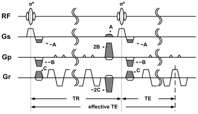
The echo-shifted InI pulse sequence. The white gradient lobes were used for the 2D EPI slice selection, phase encoding blips, and frequency encoding readouts. The gray gradient lobes were additional gradient pulses used for echo shifting.
Signal formation of echo-shifted InI
Here we derived the theoretical echo-shifted InI signal to facilitate the subsequent flip angle analysis. An echo-shifting sequence built up a coherent steady state for the transverse magnetization with the periodicity of nTR, where n denoted the number of repetitions. In our study the n = 1. According to previous studies(Chung and Duerk, 1999), the transverse magnetization in an echo shifting pulse sequence at time instant TE was
| (1) |
Here M0 denotes the longitudinal magnetization in the equilibrium and α is the flip angle. Eq.(1) allowed us to check the consistency and the discrepancy between the theoretical and the measured echo-shifted InI signals at different flip angles.
MATERIALS AND METHODS
Participants
Eight healthy participants, with normal or corrected-to-normal vision, were recruited for this study. Two of them were excluded due to the significant head movement during experiments. Informed consent for these experiments was obtained from each participant in accordance with the experimental protocol approved by the Massachusetts General Hospital Institutional Review Board.
Task
Figure 2 illustrates the paradigm design in the visual fMRI experiment. Subjects were instructed to maintain fixation at the center of a screen while viewing a high-contrast visual checkerboard contrast-reversing at 8 Hz. The checkerboard subtended 20° of visual angle and was generated from 24 evenly distributed radial wedges (15° each) and eight concentric rings of equal width. The two central concentric rings were removed. The stimuli were presented using the Presentation software (Version 14.9; Neuro Behavioral Systems, Albany, CA). The reversing checkerboard stimuli were presented for a duration of 500 ms duration and the onset of each stimulus was randomized with a minimum inter-stimulus interval of 2 seconds. Sixty stimuli were presented during eight 180-s runs, resulting in a total of 480 stimuli for each participant. Half of the visual stimuli were presented on left and the other half on the right visual hemifield. The onset time of the checkerboard stimuli on the left visual field was either synchronous or 400 ms after the MR trigger signal, which was delivered every second. Likewise, the onset time of the checkerboard presentation on the right visual field was either synchronous or 50 ms after the MR trigger signal. The timing shift of visual stimuli on left and right visual field was to test the time invariance property of the hemodynamic response function of the human visual system. In addition, a crosshair was provided in the center of the screen to assist the subjects to maintain accurate eye fixation. The cross hair was occasionally changed to an upside-down “T” for 600 ms and then changed back to a cross hair. The cross hair changes and checkerboard flashing never occurred within the same MR trigger. The participants were instructed to push a button on a response box whenever the cross hair changed, and these responses were recorded to confirm accurate performance and compliance with the task instructions.
Figure 2.
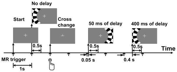
The visual task paradigm. The participants were instructed to maintain steady eye fixation on the crosshair and to push a button whenever the crosshair changed. The flashing checkerboard was presented on either left or right visual hemifield.
Echo-shifted InI acquisition
MRI data were collected with a 3T MRI scanner, using a body transmit coil and a 32-channel head array receive coil (Tim Trio, Siemens Medical Solutions, Erlangen, Germany). The array consisted of 32 circular surface coils tessellated to evenly cover the brain. The echo-shifted InI readout used EPI frequency encoding along the inferior–superior direction and phase encoding along the left–right direction after the whole-brain non-selective RF excitation. Echo-shifted InI reconstruction requires a reference scan that provides coil sensitivity maps covering the entire brain volume. Using this reference scan to construct a forward operator for spatial encoding, the accelerated acquisition replaces gradient encoding with an image reconstruction algorithm that involves solving a set of inverse problems along the anterior-posterior direction. The InI reference scan used the following imaging parameters: TR=25 ms, TE=8.2 ms (effective TE=33.2 ms), bandwidth=2894 Hz/Px; FOV 256 mm×256 mm×256 mm; 64×64×64 image matrix; flip angle = 13°. The partition phase encoding was used in the reference scan to obtain the spatial information along the anterior–posterior direction to be used as prior information in the image reconstruction. The total acquisition time for the reference scan was 12.8 s with 64 TRs allowing the coverage of a volume comprising 64 partitions with 8 repetitions. For the echo-shifted InI functional scans, we used the same volume prescription and TR, TE, flip angle, and bandwidth values as for the reference scan. The principal difference was that the partition phase encoding was removed so that a coronal projection image was obtained from each channel of the coil array. The echo-shifted InI reconstruction algorithm, described in the next section, was then used to estimate the spatial distribution of magnetization along the anterior–posterior direction. In each run, we collected 7200 measurements after 240 dummy measurements in order to reach the longitudinal magnetization steady state. A total of 8 runs of data were acquired from each participant.
In Figure 1, the gradient moment of the extra gradient pulse appearing immediately after the RF excitation in the slice-selection axis was A, which was ½ of slice-selection excitation gradient moment. The gradient moments B and C in Figure 1 used in phase and frequency encoding respectively were
| (2) |
where N denotes the number of voxels in one encoding direction (N=64 in this study), γ denotes the gyromagnetic ratio, and FOV denotes the field of view. The value of 0.75 in Eq. (2) was selected as the approximated maximal gradient strength allowed by the hardware.
Anatomical imaging
Structural MRI data for each participant were also collected in the same session using a conventional T1-weighted 3D imaging sequence (MPRAGE; TR/TE/TI = 2530/3.03/1100 ms, flip angle = 7°, partition thickness = 1.0 mm, image matrix = 256 × 224, 192 partitions, field-of-view = 25.6 cm × 22.4 cm). Using these data, the gray–white matter boundary for each participant was estimated by FreeSurfer (http://surfer.nmr.mgh.harvard.edu/) which uses an automatic segmentation algorithm to yield a triangulated mesh model with approximately 340,000 vertices (Dale et al., 1999, Fischl et al., 2001, Fischl et al., 1999). This anatomical model was then used to facilitate mapping of the structural image from native anatomical space to a standard cortical surface space (Dale et al., 1999, Fischl et al., 1999). To transform the functional results into this cortical surface space, the echo-shifted InI reference scan was spatially co-registered with the native space anatomical data using FLIRT (http://www.fmrib.ox.ac.uk/fsl), estimating a 12-parameter affine transformation between the volumetric echo-shifted InI reference and the MPRAGE anatomical space. The resulting spatial transformation was subsequently applied to each time point of the reconstructed echo-shifted InI hemodynamic estimates to spatially transform the signal estimates to a standard cortical surface space (Dale et al., 1999, Fischl et al., 1999).
Echo-shifted InI reconstruction
The raw data acquired from each channel i of the coil array was reconstructed by a standard 2D Fourier transformation, resulting in a series of complex-valued projection images. Next, we employed DRIFTER algorithm (Särkkä et al., 2012), which is a Bayesian method, to estimate and separate the physiological noise out from the fMRI signal. Unlike the widely used approach RETROICOR (Glover et al., 2000), the DRIFTER is able to track the changes in both amplitude and shape in periodic noise and separate the physiological noise from acquired data. The possible frequency estimation ranges set in DRIFTER for cardiac and respiratory noise are 0.75 Hz to 2.5 Hz and 0.083 Hz to 0.75 Hz, respectively. After the DRIFTER decomposed the fMRI signal into activation related brain signal, physiological noise and white noise, the physiological noise was subtracted from the original time course. Then we reshaped each 2D image into a vector and combined the series of image vectors into a 2D matrix Yi with the dimension of Ntime-by-[Nx×Ny], where Ntime denotes the number of acquisition time points. Nx and Ny denote the number of image pixel along the superior-inferior and the left-right directions respectively.
To reduce the temporal drift of the phase of complex-valued Yi , the phase of each pixel was corrected using a phase constraint procedure: we first simulated the 2D projection images at each channel of the coil array by synthetically summing up the 3D reference scan along the partition-encoding (anterior-posterior) direction such that the simulated echo-shifted InI acquisition , where h denotes the location indexed along partition encoding direction and r the location indexed on the image plane perpendicular to the partition encoding direction. The represents the reference scan signal of channel i with location indices r and h. The phase constraint was implemented by replacing the phase of each element in , which denotes the rth column vector of Yi , by the phase of .
After applying the phase constraint, for each channel and each pixel location in the projection data, the hemodynamic response (HDR) was separately estimated by using the standard general linear model (GLM) framework (Friston et al., 1995a, Friston et al., 1995b, Friston et al., 1995c). We used finite impulse response (FIR) basis functions to model the HDR to avoid bias in estimating the shape of the HDR. The FIR bases were temporally synchronized to the onsets of the stimuli, spanning over a 30 s period, including a 6 s pre-stimulus baseline and 24 s post-stimulus interval. Data were sampled at 40 Hz, resulting in HDR bases of 1200 temporally shifted discrete delta functions. The GLM included as model confounds constants, linear trends, and low-frequency drifts. The coefficient for each FIR basis was calculated by generalized least squares. Specifically, let denote the time-series vector of received response after applying the phase constraint and Χ denote the design matrix of the GLM. The estimated HDR basis coefficients are
| (3) |
After the GLM, the estimated HDR coefficiens br were used for volumetric spatial reconstruction. The reference scan provided the coil sensitivity map and the spatial information along the anterior-posterior direction was reconstructed. Specially, for the pixel of index r on the projection image plane, the estimated HDR coefficients from all channels of the coil array at a time instant t can be formulated as
| (4) |
where xr (t) is an nh-by-1 image vector to be reconstructed, b (t) is a nc-by-1 vector of the estimated instantaneous HDR basis coefficient, and n(t) is a nc-by-1 vector denoting the contamination noise. The matrix Ar is a nc-by-nh matrix, mapping the signals from the nh voxels of spatial index r along projection (anterior-posterior) direction to the nc-channel coil array observation. With the use of GLM residual error, the random variability between the hemodynamic responses detected by different channels of a coil array can be characterized by a noise covariance matrix C. Using the noise covariance, the forward operator Ar was then whitened to equalize the sensitivity of all channels of a coil array. Employing the singular value decomposition (SVD), the symmetric noise covariance matrix C= U Λ UH = (C1/2)(C1/2)H, where U is a complex unitary matrix and Λ is a non-negative real-valued rectangular diagonal matrix. The superscript H indicates the complex conjugate and transpose. Hence, C1/2= U Λ1/2 and C−1/2=Λ−1/2 UH. Using the whitened Ar, we have
| (5) |
where and . 〈•〉 represents the ensemble average, and Inc is an identity matrix of size nc-by-nc.
Solving the xr (t) in Eq. (5) can be an ill-posed inverse problem when the number of unknowns is larger than the observations. In order to obtain a unique solution, additional constraints need to be imposed. One common choice is the minimum-norm estimate (MNE) (Hämäläinen and Ilmoniemi, 1984):
| (6) |
where is the square of the ℓ2-norm and λ2 is a regularization parameter. The solution can be obtained by a time-invariant linear inverse operator Wr:
| (7) |
where R is a source covariance matrix. If no other spatial prior information was to be incorporated into R, then R= Inp, corresponding to a spatially uniform a priori assumption of the image contributing to the observed response. The regularization parameter can be calculated as , where ζ2 denotes the inverse of the pre-defined signal-to-noise ratio of the whitened data and tr(•) represents the trace of a matrix. Eq. (7) was repeated over 1200 time instants to reconstruct the hemodynamic response in 3D space over time.
To perform the statistical inference, the noise levels of the reconstructed volumetric images were estimated from the baseline MNE reconstruction. A baseline noise volume estimate can be calculated after defining a baseline interval, which was chosen as the interval between 0 and 6 s before the onset of the visual stimuli. Using these noise estimates, dynamic statistical parametric (dSPM) maps were derived as the ratio of the MNE reconstruction values to the baseline noise estimates at each time instant. The dSPM follows a t distribution under the null hypothesis of no hemodynamic response (Dale et al., 2000). Since the number of samples used to calculate the noise variance is large (240 in this study), the t distribution approaches the normal distribution and the t-statistics approximate the z-score.
In conventionally BOLD fMRI, brain volumes are reconstructed first followed by GLM analysis. In this study, as described above, we first performed the GLM deconvolution before volumetric reconstruction in order to reduce the dataset size and processing time, based on the assumption that these two operations commute. To verify this assumption, we tested on one participant if the order of GLM de-convolution and volumetric reconstruction was relevant, and found no substantial difference.
The temporal filter DRIFTER was employed due to the temporal instability of echo-shifted InI. Echo-shifted InI develops the steady-state free precession (SSFP) which could be disturbed by B0 fluctuation (Zhao et al., 2000). Physiological motion such as cardiac pulsation and respiration are shown to be the main sources of SSFP disturbance. The frequency of echo-shifted InI signal oscillation was the same with the frequency of physiologically induced B0 fluctuation (Zhao et al., 2000).
Temporal signal-to-noise ratio (tSNR) measurement of human brain
In fMRI, MR signal stability was restricted by multiple sources of variance, such as thermal noise or physiological noise (Bodurka et al., 2007, Kruger et al., 2001). Consequently, the Ernst angle, which provides the strongest MR signal strength for spoiled pulse sequences, did not guarantee the highest temporal SNR (tSNR), which has been shown to be a good measure of sensitivity to system instabilities and physiological signal variations (Kruger and Glover, 2001, Kruger et al., 2001, Triantafyllou et al., 2005). To examine the effect of flip angle, the flip angle was varied from 2° to 90° in 2° increments. Note that the flip angle here was nominal flip angle rather than the actual flip angle that varied across the brain due to RF field inhomogeneity. The first step of tSNR calculation was to calculate the noise covariance from the time series of resting state images. Then we spatially whitened the MR signal such that the noise signals across different channels were uncorrelated. The mean MR signal intensity of each voxel was averaged over the time series of 50 repetitive frames of signal magnitude. Likewise, the noise variation of each voxel was calculated from the variance of the time series. The voxel-wise MR signal power of each channel was combined using sum of signal powers of all channels, and noise variation was the sum of noise variances of all channels. The voxel-wise tSNR was the square root of the ratio of signal power to noise variance. Finally, the mean tSNR was averaged across gray matter image voxels. For the theoretical curve of echo-shifted InI signal magnitude, Eq. (1) was calculated with the predetermined input parameters T1, T2*, TR, TE and flip angle, and finally normalized the peak value of the theoretical curve to 1.
Actual flip angle measurement
The magnetic field experienced by spins may not be homogeneous and is influenced by several factors including the tissue dielectric constant, local chemical environment and RF wavelength. Hence, the actual flip angle after RF excitation may differ from the nominal one. To measure the difference between the actual and nominal flip angles, we progressively increased the nominal flip angle from 15° to 150° in 15° increments (Hornak et al., 1988). The nominal flip angle is controlled by the transmitted RF amplitude Arf. For every voxel, the magnitude of MR signal is a function of Arf which can be described as
| (8) |
where I denotes the MR signal intensity, ρ denotes the maximum intensity among all nominal flip angles and ρ denotes the linear relationship between RF amplitude and the actual flip angle. Since the RF amplitude is incremented through a sufficiently large range, a spatial map of actual flip angles can be found by nonlinearly fitting the measurement of I along the incremented flip angles with Eq. (8). EPI was used in this measurement and TR was set to 6 seconds.
Quantification of hemodynamic response timing
The HDR timing directly estimated from the measured hemodynamic response was considered less reliable due to the noise contamination. To reduce the noise, the measured hemodynamic response within the region of interests (ROI) was first fitted to a canonical model (Glover, 1999), and the fitted curves across the ROI image pixels were then averaged and linearly normalized such that the maximum was set to 1. In order to quantify the timing of hemodynamic response, we derived three timing indices: Onset, Time-to-Half (TTH), and Time-to-Peak (TTP). The Onset timing index is the intercept with the time axis of the fitted straight line over the rising edge of fitted hemodynamic response. (The rising edge was defined as the time course running from 10% to 90% of the peak of the fitted model.) The Time-to-Half timing index is the time reaching the mid-point of the rising edge of fitted hemodynamic response. The other timing index Time-to-Peak is the time of the peak of the fitted hemodynamic response (see Figure 3).
Figure 3.
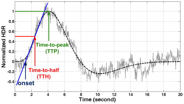
The illustration of the three timing indices: Onset, Time-to-Half (TTH) and Time-to-Peak (TTP). The gray trace represents the measured hemodynamic response. The black dashed trace represents the canonical model fitted to the measured time course. The blue line represents the line fitted to the rising edge of the canonical model.
Statistical analysis of individual-level and group-level HDR timing
For the individual-level statistical analysis, the HDRs of individual result at each ROI vertex were fitted to the canonical model after being morphed to the template brain. The timing indices associated with different stimuli onset time were calculated. Two t-tests were conducted over the ROI vertices: one of them is the paired t-test that tested whether the timing indices corresponding to different stimuli onset time was statistically distinguishable; the other t-test was to test whether the differences of timing indices were the same as the differences of visual stimuli onsets. For the group-level statistical analysis, each individual’s HDRs were averaged over ROI vertices. Then the timing indices were calculated based on the averaged HDR of each individual. The group-level statistical analysis was conducted over the timing indices of all the individuals. As in the individual-level analysis, the paired t-test was also conducted in the group level. Besides, we also calculated the confidence interval of timing indices with the probability of 0.95.
RESULTS
Reconstructed images
Since we used the 3D reference scan as the sensitivity mapping matrix, the image of MNE solution contained virtually no structural information. To facilitate the visualization, the MNE solution was added by matrix of ones and then multiplied it by the 3D reference image. The middle panel in Figure 4 shows the reconstruction of one time point of the MNE reconstruction at different axial slices. For comparison, the reference scan was also shown on the left panel. The right panel in Figure 4 shows the image of difference that represented the MNE solution. All the images shown in Figure 4 were the square root of the sum of square over all the channel images. Due to the higher coil sensitivity near the brain surface, the signal of MNE solution appeared stronger in the cortex. In other words, echo-shifted InI was more sensitive to the cortical region such as visual cortex than to the deeper brain region such as thalamus.
Figure 4.
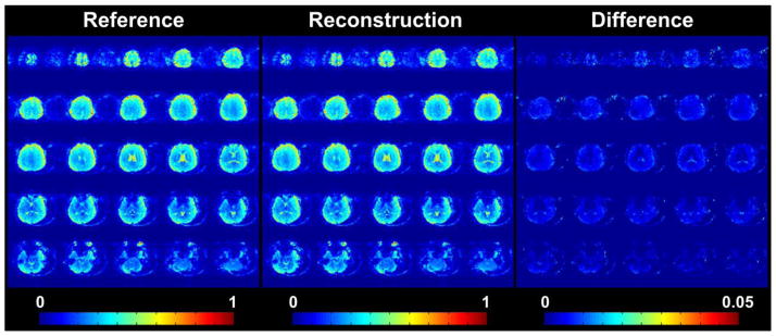
The reference, reconstructed and difference images of one single subject. The reference image is shown on the left panel. The reconstructed image is shown in the middle panel and the difference image is shown on the right panel. The signal strengths are encoded as shown in the colorbars. Please note that the dynamic range of the difference image is different from the other two images.
Flip angle analysis
Figure 5a shows the value of the transverse magnetization of gray matter measured with different nominal flip angles. This value was normalized by the maximum amplitude across all flip angles. The theoretical curve was predicted by Eq. (1) and normalized by the maximal magnetization. The theoretical curve was in good agreement with the measured curve for small flip angles. The measured and theoretical curves showed a discrepancy when the flip angles were higher than the Ernst angle of 10°. Such discrepancy has been reported and may be explained by the lack of consideration of the dispersion of resonance offset angles within one voxel in the derivation of Eq. (1) (Chung and Duerk, 1999). The other possible reason for the discrepancy might be the inaccurate operation of flip angle. Assuming the rate of inaccuracy was fixed across different nominal flip angles (e.g. 1% deviation from the nominal RF amplitude), larger nominal flip angle would cause larger phase offset. The phase offset would led to elevated baseline of SSFP signal especially when the TR was short (Zhao et al., 2000). We further calculated the tSNR of echo-shifted InI and compared with that of conventional EPI (Figure 5b). For echo-shifted InI the highest tSNR was obtained when the flip angle was around 6 degrees. This optimal flip angle may change due to the different T1 and T2* values within the gray matter ROI across subjects used in the tSNR measurements. In addition, the highest tSNR for EPI was obtained when the flip angle was 90° with TR = 2s. The tSNR ratio of EPI to echo-shifted InI was 1.71. Considering both the peak echo-shifted InI signal and the rather moderate modulation of the flip angle over tSNR, we adopted a flip angle of 13° in this study.
Figure 5.
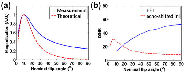
The dependence of echo-shifted InI signal and the temporal SNR (tSNR) on the nominal flip angle. (a) The theoretical (blue solid trace) and the measured (red dashed trace) amplitudes of transverse magnetization at different flip angles. The blue solid trace indicates the normalized magnetization amplitudes measured and averaged over the cortical gray matter. The red dashed trace represents the theoretical curve derived from Eq. (1). (b) The tSNR of echo-shifted InI (red dashed trace) and EPI (blue solid trace) against different flip angles.
Actual flip angle analysis
Figure 6 showed the spatial map of the difference between the actual flip angle and nominal flip angle (13°). The local B1+ field around the cortex was generally smaller than the nominal one but gradually increased when the location moved toward the center of the brain. The mean and standard deviation of flip angle difference were −0.41° and 1.55° respectively. This result supports the selected flip angle is generally valid across the whole brain.
Figure 6.

The spatial map of the difference between the actual flip angle and nominal flip angle (13°). The flip angle differences are encoded as shown in the scalebar. This map was obtained from one single subject.
Temporal and spectral analysis
The steady-state transverse magnetization in the echo-shifted InI had higher temporal instability due to motion artifacts or any imperfect gradient moment (Bernstein et al., 2004, Gibson et al., 2006). To investigate the issue of signal stability, the time course and the power spectrum of echo-shifted InI voxles averaged across the gray matter are shown in Figure 7. For comparison, the echo-shifted InI processed by DRIFTER (esInI-DRIFTER) and InI without echo shifting were also included. The temporal means of the time courses in Figure 7a were normalized to 1 in order to facilitate the comparison between three different methods. The echo-shifted InI (standard deviation = 7.2×10⁻³) was less temporally stable than InI (standard deviation = 6.3×10⁻³) (Figure 7a) and exhibited more prominent respiratory oscillations (~0.1 Hz) (Figure 7b). As for the oscillations induced by cardiac pulsation (~1.1 Hz), echo-shifted InI and InI were around the same level of signal strength (Figure 7b). However, the first harmonic of pulsation-induced physiological noise of echo-shifted InI was greatly suppressed by DRIFTER. The temporal standard deviation of esInI-DRIFTER was reduced to 6.8×10⁻³. Figure 7c demonstrated the activation maps of echo-shifted InI with and without DRIFTER. A physiologically unlikely activation site at the upper edge of the medial wall was shown in the activation map of echo-shifted InI but not in the map of esInI-DRIFTER. The HDRs of the same vertex in the visual cortex are shown in Figure 7d. The HDR of esInI-DRIFTER appeared to be more similar to the canonical model than the HDR of echo-shifted InI.
Figure 7.
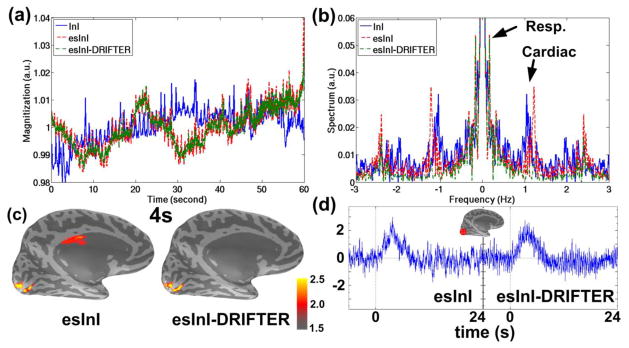
The temporal and spectral characteristics of echo-shifted InI and InI of one single subject. (a) The time courses of the InI, echo-shifted InI and esInI-DRIFTER averaged over gray matter image voxels. (b) The magnitude of the InI, echo-shifted InI and esInI-DRIFTER spectra. (c) The cortical map of statistical BOLD activation 4s after stimuli onset. Echo-shifted InI is shown on the left panel and esInI-DRIFTER on the right. (d) The time courses of echo-shifted InI (left panel) and esInI-DRIFTER (right panel) from the same vertex of the visual cortex. The center of the circled red cross indicated the location of the vertex.
Visual experiments
Figure 8 shows the group-averaged BOLD signal of the conventional EPI and the echo-shifted InI on an inflated cortical surface representation. Specifically, the top and bottom rows of Figure 8a respectively show the spatial distribution of the normalized HDR of EPI and echo-shifted InI at 4 seconds after the onset of visual stimuli presented in the right visual hemifield. The BOLD signals of both EPI and echo-shifted InI were linearly scaled to between −1 and +1. Both EPI and echo-shifted InI exhibited strong BOLD signals and similar spatial distribution in the left visual cortex when the visual stimuli were presented in the right visual hemifield. Figure 8b depicts the normalized HDRs averaged over a region of interest (ROI) defined in the left visual cortex.
Figure 8.
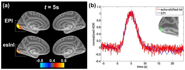
The group-averaged spatial distribution and time course of the normalized HDR of echo-shifted InI (esInI) and EPI. (a) The snapshot of the BOLD signal at 5 s after right visual stimuli onset. The BOLD activations at the gray-white matter boundary have been mapped to the cortical surface. The color scale bar encodes the normalized BOLD signal strength. (b) The normalized HDRs averaged over the visual cortex ROI in the left hemisphere, indicated by the green patch in the figure inset that, is highlighted by the dashed rectangular box in panel (a).
The stimulus-related visual cortex activity was clearly observed in the group averaged dSPM. Figure 9 shows frames of echo-shifted InI in the occipital lobe at every 25 ms. In this case, the visual stimuli were delivered to the right visual hemifield. These frames show progressively increasing BOLD signal starting at 3 s after the stimuli onset. The signal decreased to baseline approximately 7 s after the stimuli onset. Taken together, the data in Figure 9 suggests that echo-shifted InI can provide spatiotemporal characterization of BOLD signal of human visual cortex with unprecedented temporal resolution.
Figure 9.
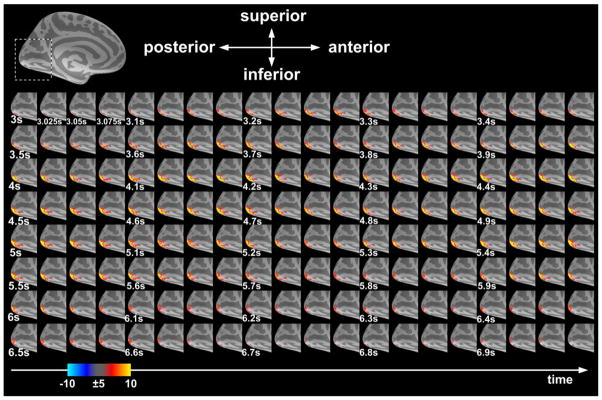
The group-averaged snapshots of the left hemispheric visual cortex dSPMs acquired by echo-shifted InI. At the top of the figure, the dashed rectangular box indicates the ROI in the left inflated cortical surface. The color bar shows the z-statistics of BOLD activations.
In the timing analysis, the ROI-averaged HDRs of each individual are shown in Figure 10. The timing axis is with respect to the onset of MR trigger. The HDRs in Figure 10a were evoked by right visual-hemifield stimuli that were either 0 ms or 50 ms lagged behind the MR trigger. Similarly, the HDRs in Figure 10b were evoked by left visual-hemifield stimuli that were either 0 ms or 400 ms lagged behind the MR trigger. All the HDRs were normalized by the peak values of the fitting curves. The timing differences between the blue and red traces in Figure 10b are generally larger than the timing differences in Figure 10a, which is consistent with the larger shift of stimuli onset time in Figure 10b. The individual-level statistical results are listed in Table 1. The results marked in red indicate not only that the HDRs corresponding to the different stimulus-onset shifts are temporally distinguishable but also that the timing differences between HDRs were statistically similar to the stimuli onset latency. Table 1b shows that 83% (5 out of 6) of the individual testing results of latency differences in the Time-to-Half columns were statistically distinguishable (values marked red). The results suggested that echo-shifted InI was able to differentiate between the HDRs with stimuli onset latency of at least 400 ms and the estimation of the timing differences was statistically similar to 400 ms in the individual level. No statistical results were marked in red in Table 1a because the temporal variation across vertices in each individual was higher than 50 ms. Nevertheless, 83% of the timing indices in Table 1a were statistically similar to 50 ms.
Figure 10.
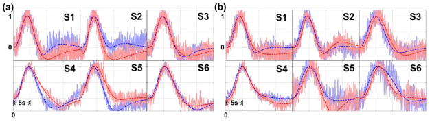
The normalized HDRs and fitting curves of each individual. The individuals were indexed from S1 to S6. (a) The HDR corresponding to the visual stimuli with no delay (blue) vs. 50-ms delay (red). (b) The HDR corresponding to the visual stimuli with no delay (blue) vs. 400-ms delay (red). The solid traces indicated the measured data and the dashed traces indicated the fitting curves.
Table 1.
The results of hypothesis testing in the individual level. (a) The testing results associated with stimuli time shift = 50 ms. (b) The testing results associated with stimuli time shift = 400 ms. τ50 and τ400 indicate the difference on timing indices associated with stimuli time shifts of 50 ms and 400 ms, respectively.
| (a) | Onset | Time-To-Half | Time-To-Peak | |||
|---|---|---|---|---|---|---|
| Hypothesis test | τ50 = 0? | τ50 = 50? | τ50 = 0? | τ50 = 50? | τ50 = 0? | τ50 = 50? |
| S1 | Y (p=0.096) | Y (p=0.193) | Y (p=0.286) | Y (p=0.818) | Y (p=0.355) | Y (p=0.148) |
| S2 | N (p<0.001) | N (p<0.001) | Y (p=0.491) | Y (p=0.919) | N (p<0.001) | N (p<0.001) |
| S3 | Y (p=0.250) | Y (p=0.434) | Y (p=0.311) | Y (p=0.673) | Y (p=0.487) | Y (p=0.122) |
| S4 | Y (p=0.737) | Y (p=0.987) | Y (p=0.728) | Y (p=0.935) | Y (p=0.618) | Y (p=0.739) |
| S5 | Y (p=0.503) | Y (p=0.255) | Y (p=0.221) | Y (p=0.477) | N (p<0.001) | N (p<0.001) |
| S6 | Y (p=0.073) | Y (p=0.147) | Y (p=0.142) | Y (p=0.240) | Y (p=0.280) | Y (p=0.404) |
| (b) | Onset | Time-To-Half | Time-To-Peak | |||
| Hypothesis test | τ400 = 0? | τ400 = 400? | τ400 = 0? | τ400 = 400? | τ400 = 0? | τ400 = 400? |
| S1 | N (p<0.001) | Y (p=0.164) | N (p<0.001) | Y (p=0.310) | N (p=0.030) | N (p<0.001) |
| S2 | N (p<0.001) | Y (p=0.175) | N (p<0.001) | Y (p=0.055) | N (p=0.002) | Y (p=0.924) |
| S3 | N (p<0.001) | N (p<0.001) | N (p<0.001) | N (p<0.001) | N (p<0.001) | N (p=0.003) |
| S4 | N (p=0.006) | Y (p=0.566) | N (p=0.009) | Y (p=0.902) | Y (p=0.194) | Y (p=0.116) |
| S5 | Y (p=0.087) | Y (p=0.603) | N (p=0.032) | Y (p=0.393) | N (p=0.005) | Y (p=0.466) |
| S6 | Y (p=0.168) | Y (p=0.679) | N (p=0.049) | Y (p=0.564) | Y (p=0.110) | Y (p=0.885) |
The testing results highlighted in red demonstrate τ50 and τ400 values that were statistically significantly distinguishable (τ>0) and statistically similar to the stimuli onset latency.
Figure 11 shows the averaged HDR and fitting curves across the individuals. Figure 11a is associated with the stimuli onset latency of 50 ms. The timing differences of Onset, Time-to-Half, and Time-to-Peak were 218 ms, 121 ms and 64 ms respectively. The timing differences of Time-to-Half, and Time-to-Peak were statistically similar to 50 ms (p=0.100, p=0.911 respectively). Figure 11b is associated with the stimuli onset latency of 400 ms. In Figure 11b, likewise, the timing differences of Onset, Time-to-Half, and Time-to-Peak were 609 ms, 562 ms and 312 ms respectively. All the timing differences in terms of Onset, Time-to-Half, and Time-to-Peak were statistically similar to 400 ms of stimuli onset latency (p=0.054, p=0.061, p=0.435 respectively). The group-level statistical results are shown in Table 2. When the stimuli onset latency was 50 ms, the paired t-test results of Onset, Time-to-Half, and Time-to-Peak were p=0.016, p=0.019 and p=0.618 respectively. The confidence intervals of the mean with probability of 95% in terms of Onset, Time-to-Half, and Time-to-Peak were -246 ms to 374 ms, 30 ms to 212 ms and 62 ms to 375 ms. The stimuli onset latency of 50 ms was within the confidence intervals of Onset and Time-To-Half. On the other hand, when the stimuli onset latency was 400 ms, the paired t-test results of Onset, Time-to-Half, and Time-to-Peak were p<0.001, p<0.001 and p=0.03 respectively. The confidence intervals of the mean with probability of 95% in terms of Onset, Time-to-Half, and Time-to-Peak were 395 ms to 823 ms, 390 ms to 735 ms and 46 ms to 578 ms. The stimuli onset latency of 400 ms was within the confidence intervals of all timing indices. The statistical results suggested that echo-shifted InI was able to differentiate between the HDRs and estimate the stimuli onset latency with the time difference as short as 50 ms at group level.
Figure 11.
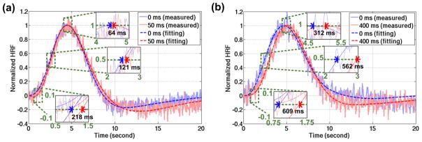
The group-averaged HDRs and fitting curves. (a) HDR timing measures to visual stimuli with no delay (blue) vs. 50-ms delay (red). (b) HDR timing measures to visual stimuli with no delay (blue) vs. a 400-ms delay (red). In both figures (a, b), the solid traces with lighter color represented the measured data and the dashed traces represented the fitted model. The three insets in each panel were enlarged for better visualization on Onset, Time-to-Half, and Time-to-Peak.
Table 2.
The results of timing analysis in the group level. The p-values were from the hypothesis testing that the mean of timing index was equal to 0.
| Time shift | Onset | Timt-To-Half | Time-To-peak | |||
|---|---|---|---|---|---|---|
| mean | CI (95%) | mean | CI (95%) | mean | CI (95%) | |
| 50 ms | 218 ms (p=0.016) | 62ms to 375 ms | 121 ms (p=0.019) | 30 ms to 212 ms | 64 ms (p=0.618) | −246 ms to 374 ms |
| 400 ms | 609 ms (p<0.001) | 395 ms to 823 ms | 562 ms (p<0.001) | 390 ms to 735 ms | 312 ms (p=0.03) | 46 ms to578 ms |
The CI denotes confidence interval of mean with the probability of 0.95.
Finally, echo-shifted InI turns off the fat suppression otherwise the dephased gradient moment cannot be refocused. As a consequence, the fat signal of the scalp would appear on the brain as Nyquist ghost artifact. However, the static fat signal had minimum effect on the dynamic functional response in the present result. As shown in the Figure 12a, the bright fat signal was aliased in the visual cortex. Nevertheless, the aliased voxels showed the BOLD activation normally. The voxel enclosed by the blue square block also had normal HDR as shown in Figure 12b.
Figure 12.
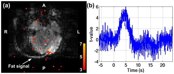
The statistical map and HDR of BOLD activation of one single subject while the aliased fat signal was presented. (a) The statistical map 4s after the right visual stimuli onset. (b) The HDR of the voxel enclosed by the blue block in (a).
DISCUSSION
The echo shifting technique was first developed to make rapid T2* weighted imaging available on standard clinical scanners (van Gelderen et al., 2012), such as fMRI based on BOLD contrast (Duyn et al., 1994) and MR thermometry (Chung et al., 1999, de Zwart et al., 1996, Harth et al., 1997). In our previous work, echo shifting technique has been used in 2D single-slice InI to achieve 20 ms of acquisition time (Lin et al., 2006). The challenge for the 2D method is that one needs to know where the activation is located prior to the experiment. This study extends the previous version of 2D method to a 3D method that allows obtaining a whole brain volume in a single shot.
A T2*-weighted 3D imaging with echo shifting has been introduced as PRESTO-SENSE, which has temporal resolution of 500 ms per brain volume and voxel size of 4×4×4 mm3(Klarhofer et al., 2003). Unlike the PRESTO-SENSE, which may accelerate the acquisition by a factor of 2 along the phase encoding direction, echo-shifted InI reduces the scanning time by 64-fold without the compromise of voxel size. Compared with echo-shifted InI, these multi-slice techniques may be more prone to inflow effects than the present echo-shifted InI approach with 3D encoding (Duyn et al., 1994b). In addition, multi-slice excitation, which combines all the slices into one image, incurs the shot-to-shot phase instability, potentially adding to signal fluctuation (van Gelderen et al., 2012). On the contrary, volume acquisition is free from such effects because of the single shot approach.
Although our results suggest that echo-shifted InI has no shot-to-shot phase instability within one volume, echo-shifted InI seemed to be temporally instable across volumes, as the know property of steady-state coherent pulse sequence. Our empirical data suggests that the temporal instability of echo-shifted InI was 14.3% higher than that of InI. The spectrum analysis showed that most of the temporal variation came from the respiratory and cardiac oscillation. However, this problem could be alleviated by employing the temporal filtering technique DRIFTER (Särkkä et al., 2012). The DRIFTER suppressed the physiological noise and hereby not only increased the spatial stability of BOLD activation map but also the temporal stability of HDR. One of the other possible sources of temporal instability is the dynamic inaccuracy of system operation, such as non-ideal gradient strength or flip angle. If the temporal pattern of inaccurate system operation is non-periodic, the DRIFTER can barely reduce the temporal instability. However, as shown in Figure 7b, the noise floor of echo-shifted InI was in the same level with InI. Hence, the empirical data did not suggest that the dynamic imperfect system realization would cause echo-shifted InI more temporal instable than InI.
In the timing analysis, we used Onset, Time-to-Half and Time-to-Peak to quantify the activation time of evoked hemodynamic responses. The capability of echo-shifted InI in detecting the timing difference of HDR was tested in the individual level and group level. The results suggested that echo-shift InI could detect the timing difference in the individual level when the HDRs were 400 ms apart. The echo-shifted InI might not be able to detect the timing difference as small as 50 ms because the temporal variation of HDR was higher than that. However, our data suggested that such temporal variation could be reduced after group average (n=6) so that the timing difference of 50 ms was detectable to the echo-shifted InI in the group level. Additionally, to demonstrate that volumetric scan time of 25 ms was required for such detection capability, we sub-sampled the HDRs to the temporal resolution of 100 ms, 400 ms and 1s and then analyzed the timing differences in group level. The results listed in Table 3 suggested that the variation of timing indices increased as the temporal resolution decreased. Therefore, the high temporal resolution of echo-shifted InI was important for reliable detection of timing difference.
Table 3.
The group-level timing indices when the temporal resolutions were 25 ms, 100 ms, 400 ms and 1s.
| Scan time | Time shift = 50 ms | Time shift = 400 ms | ||||
|---|---|---|---|---|---|---|
| Onset | TTH | TTP | Onset | TTH | TTP | |
| 25 ms | μ= 218 ms σ= 61 ms |
μ= 121 ms σ= 35 ms |
μ= 64 ms σ= 121 ms |
μ= 609 ms σ= 83 ms |
μ= 562 ms σ= 67 ms |
μ= 312 ms σ= 103 ms |
| 100 ms | μ= 170 ms σ= 100 ms |
μ= 88 ms σ= 55 ms |
μ= 40 ms σ= 135 ms |
μ= 646 ms σ= 100 ms |
μ= 636 ms σ= 56 ms |
μ= 396 ms σ= 124 ms |
| 400 ms | μ= 40 ms σ= 197 ms |
μ= 18 ms σ= 130 ms |
μ= −72 ms σ= 139 ms |
μ= 539 ms σ= 165 ms |
μ= 459 ms σ= 103 ms |
μ= 236 ms σ= 261 ms |
| 1 s | μ= 9 ms σ= 175 ms |
μ= −79 ms σ= 209 ms |
μ=−103 ms σ= 234 ms |
μ= 283 ms σ= 312 ms |
μ= 411 ms σ= 178 ms |
μ= 441 ms σ= 173 ms |
The μ, σ denotes the mean of timing index and its standard deviation, respectively.
Although it was premature to conclude from our data which timing index was the most accurate one, the timing index Time-To-Half performed generally better in the detection of timing difference in either individual or group level. Onset, by definition, was calculated from 10% to 90% of the peak of the fitted model. Therefore the random noise that fluctuated over 10% in the baseline, which usually was the case, might affect the accuracy of Onset. Time-To-Peak, on the other hand, was picked at a relatively late stage when the bottom-up serial processing order might already be partially confounded by top-down (countercurrent) feedback.
The dephasing magnetization immediately after the RF excitation in the first TR period and then refocusing by the other gradient lobes in the second TR period (gradient lobes A, B and C in Figure 1) can impose some diffusion weighting. To check how much diffusion weighting was introduced into the echo-shifted InI images, we calculated the associated b-value (Le Bihan, 1995). Ignoring the diffusion weighting due to the frequency and phase encoding gradient moments, the b-value of the echo-shifted InI was 2G2δ2(TR − δ), where G denoted the strength of dephasing gradient and δ denoted the pulse duration of dephasing gradient. This formulation is similar to the b-value corresponding to bipolar gradient (Stejskal and Tanner, 1965) which was formulated as γ2G2δ2(Δ − δ/ 3), where Δ denoted the spacing of the two bipolar gradients. With G = 18.713 mT/m and δ =0.24 ms in our study, the b-value of echo-shifted InI was approximately equal to 0.0009 s/mm2, which caused negligible diffusion attenuation effect.
In contrast to the high temporal resolution of echo-shifted InI, its spatial resolution was limited to the number of independent information from the coil array. Besides, the level of point spreading that depended on the chosen reconstruction methods determined spatial resolution. In this study we employed the MNE in the image reconstruction process. Consistent with our previous submissions and publications (Lin et al., 2010, Lin et al., 2008b), we found that the spatial resolution is ~5 mm at the cortex, while in the subcortical area the spatial resolution was about 12~16 mm (see Figure 13 in the APPENDIX). For studies on cortical activity, the spatial resolution was adequate. For studies involving deeper brain regions, additional techniques that reconstruct images with less compromise in spatial resolution may need to be used. One possible strategy to improve the spatial resolution was to make more sophisticated use of the spatial information, such as reconstructing the images in frequency domain instead of in the image domain (Lin et al., 2010) or using spatial filtering (Lin et al., 2008b, Liou et al., 2011). Yet another strategy is to acquire different projection images over repetitive measurements and subsequently to reconstruct images using concatenated data (Wen-Kai Tsai et al., 2012). However, it is true that our method should not be used in fMRI experiments where high spatial resolution is required.
Figure 13.

The PSF across the whole brain when MNE was used for spatial reconstruction. The unit is millimeter. Higher PSF value means lower spatial resolution.
As a consequence of acceleration along the projection direction, motion correction was difficult to be applied on the series of projection images. Hence, instantaneous InI reconstruction can be useful provided 1) the reference scan was satisfactory and 2) there is minimal motion between the instantaneous InI measurement and the reference scan measurement. Even the two above-mentioned assumptions stand, the instantaneous InI reconstruction can still have a lower resolution than the reference scan because any dynamic information different from the reference scan, including noise and signal, will be spatially smeared as the consequence of using the constraint to minimize the error quantified by the ℓ2-norm.
In summary, our data suggest that echo-shifted InI may help achieve an unprecedented fMRI sampling rate of one brain volume per 25 ms with the nominal spatial resolution of 4×4×4 mm3. By employing the principle of echo shifting, we were able to obtain BOLD data with a TR shorter than the TE, which was required to achieve the optimal BOLD contrast. The effect of nominal flip angle on the echo-shifted InI was explored in terms of MR signal strength and tSNR. The measured curve of echo-shifted InI signal strength against different flip angles was generally consistent with the curve predicted by the equation derived in previous studies (Chung and Duerk, 1999). Compared with conventional EPI, which allows whole-brain acquisitions in 2 seconds, echo-shifted InI provided 80-fold speedup with less than 2-fold tSNR loss. The capabilities of echo-shifted InI were investigated by testing whether the time shift of visual stimuli in millisecond scale could be detected based on the time courses of hemodynamic responses at visual cortex. According to the experimental results, echo-shifted InI could detect the hemodynamic responses timing difference of 400 ms at individual level. After group average, echo-shifted InI could detect the timing difference as small as 50 ms. Taken together, we hope that echo-shifted InI can be a useful tool for future investigations of hemodynamic timing in cortical and subcortical areas.
Highlights.
The shortest TR in steady state incoherent pulse sequences is constrained by the optimal TE for BOLD contrast (~30 ms at 3T).
Echo-shifted InI integrates the echo shifting and InI techniques to measure BOLD fMRI at a sampling rate of one volume per 25 ms with whole brain coverage.
Compared with EPI, the echo-shifted InI provides 80-fold speedup with similar spatial resolution and less than 2-fold temporal SNR loss.
Using the echo-shifted InI, the hemodynamic responses at the human visual cortex corresponding to different stimuli onset latencies demonstrate similar time shift.
Acknowledgments
We appreciate the technical support by Mary T. O’Hara and Lawrence T. Whiteat Athinoula A. Martinos Center for Biomedical Imaging. This work was supported in part by the An-Yi Hung and Stephanie Rossi. Additionally, this work was supported by National Institutes of Health (NIH) Grants R01DA14178, R01MH083744, R21DC010060, R01HD040712, R01NS037462, P41 RR14075, R01EB006847, RO1EB000790, R21EB007298, the Mental Illness and Neuroscience Discovery Institute (MIND), NSC 100-2917-I-564-027 (National Science Council, Taiwan), NSC 101-2628-B-002-005-MY3 (National Science Council, Taiwan), 100-EC-17-A-19-S1-175 (Ministry of Economic Affairs, Taiwan), NHRI-EX102-10247EI (National Health Research Institute, Taiwan), and Academy of Finland (the FiDiPro program and grant 127624), Finnish Cultural Foundation, and Finnish Foundation for Technology Promotion. The research environment was supported by NIH/National Center for Research Resources Shared Instrumentation Grants S10RR014978, S10RR021110, S10RR019307, and S10RR023401.
APPENDIX.
This study employed MNE for the spatial reconstruction of echo-shifted InI. The performance of the reconstruction can be quantified using similar procedure in MEG source analysis (Chang et al., 2010). The spatial resolution can be estimated by calculating the point spread function (PSF) at each location as
| (8) |
where denotes the distance between the true source at the location of the hth element of the column vector xr and the source estimate at the location of the h′th element of the column vector xr. denotes the source estimate at the location of the h′th element of the column vector xr while the true source is at the location of hth element of the column vector xr. PSFrh is the point spread at the location of the hth element of the column vector xr.
Figure 13 shows the PSF map across the whole brain. As expected, the spatial resolution at the cortex is close to the voxel size. However, the spatial resolution became lower at deeper brain regions.
Footnotes
Publisher's Disclaimer: This is a PDF file of an unedited manuscript that has been accepted for publication. As a service to our customers we are providing this early version of the manuscript. The manuscript will undergo copyediting, typesetting, and review of the resulting proof before it is published in its final citable form. Please note that during the production process errors may be discovered which could affect the content, and all legal disclaimers that apply to the journal pertain.
RFERENCES
- Belliveau J, Kennedy D, McKinstry R, Buchbinder B, Weisskoff R, Cohen M, Vevea J, Brady T, Rosen B. Functional mapping of the human visual cortex by magnetic resonance imaging. Science. 1991;254:716–719. doi: 10.1126/science.1948051. [DOI] [PubMed] [Google Scholar]
- Bernstein MA, King KF, Zhou ZJ. Handbook of MRI pulse sequences. Amsterdam ; Boston: Academic Press; 2004. [Google Scholar]
- Blum MJ, Braun M, Rosenfeld D. Fast magnetic resonance imaging using spiral trajectories. Australas Phys Eng Sci Med. 1987;10:79–87. [PubMed] [Google Scholar]
- Bodurka J, Ye F, Petridou N, Murphy K, Bandettini PA. Mapping the MRI voxel volume in which thermal noise matches physiological noise--implications for fMRI. Neuroimage. 2007;34:542–549. doi: 10.1016/j.neuroimage.2006.09.039. [DOI] [PMC free article] [PubMed] [Google Scholar]
- Chang WT, Nummenmaa A, Hsieh JC, Lin FH. Spatially sparse source cluster modeling by compressive neuromagnetic tomography. Neuroimage. 2010;53:146–160. doi: 10.1016/j.neuroimage.2010.05.013. [DOI] [PMC free article] [PubMed] [Google Scholar]
- Chung YC, Duerk JL. Signal formation in echo-shifted sequences. Magn Reson Med. 1999;42:864–875. doi: 10.1002/(sici)1522-2594(199911)42:5<864::aid-mrm5>3.0.co;2-8. [DOI] [PubMed] [Google Scholar]
- Chung YC, Duerk JL, Shankaranarayanan A, Hampke M, Merkle EM, Lewin JS. Temperature measurement using echo-shifted FLASH at low field for interventional MRI. J Magn Reson Imaging. 1999;9:138–145. doi: 10.1002/(sici)1522-2586(199901)9:1<138::aid-jmri18>3.0.co;2-a. [DOI] [PubMed] [Google Scholar]
- Dale AM, Fischl B, Sereno MI. Cortical surface-based analysis. I. Segmentation and surface reconstruction. Neuroimage. 1999;9:179–194. doi: 10.1006/nimg.1998.0395. [DOI] [PubMed] [Google Scholar]
- Dale AM, Liu AK, Fischl BR, Buckner RL, Belliveau JW, Lewine JD, Halgren E. Dynamic statistical parametric mapping: combining fMRI and MEG for high-resolution imaging of cortical activity. Neuron. 2000;26:55–67. doi: 10.1016/s0896-6273(00)81138-1. [DOI] [PubMed] [Google Scholar]
- de Zwart JA, van Gelderen P, Kelly DJ, Moonen CT. Fast magnetic-resonance temperature imaging. Journal of magnetic resonance Series B. 1996;112:86–90. doi: 10.1006/jmrb.1996.0115. [DOI] [PubMed] [Google Scholar]
- Duyn JH, Mattay VS, Sexton RH, Sobering GS, Barrios FA, Liu G, Frank JA, Weinberger DR, Moonen CT. 3-dimensional functional imaging of human brain using echo-shifted FLASH MRI. Magn Reson Med. 1994;32:150–155. doi: 10.1002/mrm.1910320123. [DOI] [PubMed] [Google Scholar]
- Feinberg DA, Moeller S, Smith SM, Auerbach E, Ramanna S, Gunther M, Glasser MF, Miller KL, Ugurbil K, Yacoub E. Multiplexed echo planar imaging for sub-second whole brain FMRI and fast diffusion imaging. PloS one. 2010;5:e15710. doi: 10.1371/journal.pone.0015710. [DOI] [PMC free article] [PubMed] [Google Scholar]
- Fischl B, Liu A, Dale AM. Automated manifold surgery: constructing geometrically accurate and topologically correct models of the human cerebral cortex. IEEE Trans Med Imaging. 2001;20:70–80. doi: 10.1109/42.906426. [DOI] [PubMed] [Google Scholar]
- Fischl B, Sereno MI, Dale AM. Cortical surface-based analysis. II: Inflation, flattening, and a surface-based coordinate system. Neuroimage. 1999;9:195–207. doi: 10.1006/nimg.1998.0396. [DOI] [PubMed] [Google Scholar]
- Friston KJ, Frith CD, Frackowiak RS, Turner R. Characterizing dynamic brain responses with fMRI: a multivariate approach. Neuroimage. 1995a;2:166–172. doi: 10.1006/nimg.1995.1019. [DOI] [PubMed] [Google Scholar]
- Friston KJ, Frith CD, Turner R, Frackowiak RS. Characterizing evoked hemodynamics with fMRI. Neuroimage. 1995b;2:157–165. doi: 10.1006/nimg.1995.1018. [DOI] [PubMed] [Google Scholar]
- Friston KJ, Holmes AP, Poline JB, Grasby PJ, Williams SC, Frackowiak RS, Turner R. Analysis of fMRI time-series revisited. Neuroimage. 1995c;2:45–53. doi: 10.1006/nimg.1995.1007. [DOI] [PubMed] [Google Scholar]
- Gibson A, Peters AM, Bowtell R. Echo-shifted multislice EPI for high-speed fMRI. Magn Reson Imaging. 2006;24:433–442. doi: 10.1016/j.mri.2005.12.030. [DOI] [PubMed] [Google Scholar]
- Glover GH. Deconvolution of impulse response in event-related BOLD fMRI. Neuroimage. 1999;9:416–429. doi: 10.1006/nimg.1998.0419. [DOI] [PubMed] [Google Scholar]
- Glover GH, Li TQ, Ress D. Image-based method for retrospective correction of physiological motion effects in fMRI: RETROICOR. Magn Reson Med. 2000;44:162–167. doi: 10.1002/1522-2594(200007)44:1<162::aid-mrm23>3.0.co;2-e. [DOI] [PubMed] [Google Scholar]
- Griswold MA, Jakob PM, Heidemann RM, Nittka M, Jellus V, Wang J, Kiefer B, Haase A. Generalized autocalibrating partially parallel acquisitions (GRAPPA) Magn Reson Med. 2002;47:1202–1210. doi: 10.1002/mrm.10171. [DOI] [PubMed] [Google Scholar]
- Hämäläinen M, Ilmoniemi R. Interpreting measured magnetic fields of the brain: estimates of curent distributions. Helsinki University of Technology; Helsinki, Finland: 1984. [Google Scholar]
- Harth T, Kahn T, Rassek M, Schwabe B, Schwarzmaier HJ, Lewin JS, Modder U. Determination of laser-induced temperature distributions using echo-shifted TurboFLASH. Magn Reson Med. 1997;38:238–245. doi: 10.1002/mrm.1910380212. [DOI] [PubMed] [Google Scholar]
- Hennig J, Zhong K, Speck O. MR-Encephalography: Fast multi-channel monitoring of brain physiology with magnetic resonance. Neuroimage. 2007;34:212–219. doi: 10.1016/j.neuroimage.2006.08.036. [DOI] [PubMed] [Google Scholar]
- Hornak JP, Szumowski J, Bryant RG. Magnetic field mapping. Magn Reson Med. 1988;6:158–163. doi: 10.1002/mrm.1910060204. [DOI] [PubMed] [Google Scholar]
- Klarhofer M, Dilharreguy B, van Gelderen P, Moonen CT. A PRESTO-SENSE sequence with alternating partial-Fourier encoding for rapid susceptibility-weighted 3D MRI time series. Magn Reson Med. 2003;50:830–838. doi: 10.1002/mrm.10599. [DOI] [PubMed] [Google Scholar]
- Kruger G, Glover GH. Physiological noise in oxygenation-sensitive magnetic resonance imaging. Magn Reson Med. 2001;46:631–637. doi: 10.1002/mrm.1240. [DOI] [PubMed] [Google Scholar]
- Kruger G, Kastrup A, Glover GH. Neuroimaging at 1.5 T and 3.0 T: comparison of oxygenation-sensitive magnetic resonance imaging. Magn Reson Med. 2001;45:595–604. doi: 10.1002/mrm.1081. [DOI] [PubMed] [Google Scholar]
- Kwong KK, Belliveau JW, Chesler DA, Goldberg IE, Weisskoff RM, Poncelet BP, Kennedy DN, Hoppel BE, Cohen MS, Turner R, et al. Dynamic magnetic resonance imaging of human brain activity during primary sensory stimulation. Proc Natl Acad Sci U S A. 1992;89:5675–5679. doi: 10.1073/pnas.89.12.5675. [DOI] [PMC free article] [PubMed] [Google Scholar]
- Le Bihan D. Diffusion and perfusion magnetic resonance imaging : applications to functional MRI. New York: Raven Press; 1995. [Google Scholar]
- Lee HL, Zahneisen B, Hugger T, Levan P, Hennig J. Tracking dynamic resting-state networks at higher frequencies using MR-encephalography. NeuroImage. 2012;65C:216–222. doi: 10.1016/j.neuroimage.2012.10.015. [DOI] [PubMed] [Google Scholar]
- Lin FH, Huang TY, Chen NK, Wang FN, Stufflebeam SM, Belliveau JW, Wald LL, Kwong KK. Functional MRI using regularized parallel imaging acquisition. Magn Reson Med. 2005;54:343–353. doi: 10.1002/mrm.20555. [DOI] [PMC free article] [PubMed] [Google Scholar]
- Lin FH, Nummenmaa A, Witzel T, Polimeni JR, Zeffiro TA, Wang FN, Belliveau JW. Physiological noise reduction using volumetric functional magnetic resonance inverse imaging. Hum Brain Mapp. 2011 doi: 10.1002/hbm.21403. [DOI] [PMC free article] [PubMed] [Google Scholar]
- Lin FH, Tsai KW, Chu YH, Witzel T, Nummenmaa A, Raij T, Ahveninen J, Kuo WJ, Belliveau JW. Ultrafast inverse imaging techniques for fMRI. Neuroimage. 2012 doi: 10.1016/j.neuroimage.2012.01.072. [DOI] [PMC free article] [PubMed] [Google Scholar]
- Lin FH, Wald LL, Ahlfors SP, Hamalainen MS, Kwong KK, Belliveau JW. Dynamic magnetic resonance inverse imaging of human brain function. Magn Reson Med. 2006;56:787–802. doi: 10.1002/mrm.20997. [DOI] [PubMed] [Google Scholar]
- Lin FH, Witzel T, Chang WT, Wen-Kai Tsai K, Wang YH, Kuo WJ, Belliveau JW. K-space reconstruction of magnetic resonance inverse imaging (K-InI) of human visuomotor systems. Neuroimage. 2010;49:3086–3098. doi: 10.1016/j.neuroimage.2009.11.016. [DOI] [PMC free article] [PubMed] [Google Scholar]
- Lin FH, Witzel T, Mandeville JB, Polimeni JR, Zeffiro TA, Greve DN, Wiggins G, Wald LL, Belliveau JW. Event-related single-shot volumetric functional magnetic resonance inverse imaging of visual processing. Neuroimage. 2008a;42:230–247. doi: 10.1016/j.neuroimage.2008.04.179. [DOI] [PMC free article] [PubMed] [Google Scholar]
- Lin FH, Witzel T, Zeffiro TA, Belliveau JW. Linear constraint minimum variance beamformer functional magnetic resonance inverse imaging. Neuroimage. 2008b;43:297–311. doi: 10.1016/j.neuroimage.2008.06.038. [DOI] [PMC free article] [PubMed] [Google Scholar]
- Liou ST, Witzel T, Numenmaa A, Chang WT, Tsai KW, Kuo WJ, Chung HW, Lin FH. Functional magnetic resonance inverse imaging of human visuomotor systems using eigenspace linearly constrained minimum amplitude (eLCMA) beamformer. Neuroimage. 2011;55:87–100. doi: 10.1016/j.neuroimage.2010.11.072. [DOI] [PMC free article] [PubMed] [Google Scholar]
- Liu G, Sobering G, Duyn J, Moonen CT. A functional MRI technique combining principles of echo-shifting with a train of observations (PRESTO) Magn Reson Med. 1993;30:764–768. doi: 10.1002/mrm.1910300617. [DOI] [PubMed] [Google Scholar]
- Logothetis NK, Pauls J, Augath M, Trinath T, Oeltermann A. Neurophysiological investigation of the basis of the fMRI signal. Nature. 2001;412:150–157. doi: 10.1038/35084005. [DOI] [PubMed] [Google Scholar]
- Mansfield P. Multi-planar image formation using NMR spin echoes. Journal of Physics C: Solid State Physics. 1977;10:55–L58. [Google Scholar]
- McGibney G, Smith MR, Nichols ST, Crawley A. Quantitative evaluation of several partial Fourier reconstruction algorithms used in MRI. Magn Reson Med. 1993;30:51–59. doi: 10.1002/mrm.1910300109. [DOI] [PubMed] [Google Scholar]
- Menon RS, Luknowsky DC, Gati JS. Mental chronometry using latency-resolved functional MRI. Proc Natl Acad Sci U S A. 1998;95:10902–10907. doi: 10.1073/pnas.95.18.10902. [DOI] [PMC free article] [PubMed] [Google Scholar]
- Menon RS, Ogawa S, Tank DW, Ugurbil K. Tesla gradient recalled echo characteristics of photic stimulation-induced signal changes in the human primary visual cortex. Magn Reson Med. 1993;30:380–386. doi: 10.1002/mrm.1910300317. [DOI] [PubMed] [Google Scholar]
- Moonen CT, Liu G, van Gelderen P, Sobering G. A fast gradient-recalled MRI technique with increased sensitivity to dynamic susceptibility effects. Magn Reson Med. 1992;26:184–189. doi: 10.1002/mrm.1910260118. [DOI] [PubMed] [Google Scholar]
- Ogawa S, Lee TM, Kay AR, Tank DW. Brain magnetic resonance imaging with contrast dependent on blood oxygenation. Proc Natl Acad Sci U S A. 1990;87:9868–9872. doi: 10.1073/pnas.87.24.9868. [DOI] [PMC free article] [PubMed] [Google Scholar]
- Ogawa S, Lee TM, Stepnoski R, Chen W, Zhu XH, Ugurbil K. An approach to probe some neural systems interaction by functional MRI at neural time scale down to milliseconds. Proc Natl Acad Sci U S A. 2000;97:11026–11031. doi: 10.1073/pnas.97.20.11026. [DOI] [PMC free article] [PubMed] [Google Scholar]
- Ohliger MA, Grant AK, Sodickson DK. Ultimate intrinsic signal-to-noise ratio for parallel MRI: electromagnetic field considerations. Magn Reson Med. 2003;50:1018–1030. doi: 10.1002/mrm.10597. [DOI] [PubMed] [Google Scholar]
- Parrish TB, Gitelman DR, LaBar KS, Mesulam MM. Impact of signal-to-noise on functional MRI. Magn Reson Med. 2000;44:925–932. doi: 10.1002/1522-2594(200012)44:6<925::aid-mrm14>3.0.co;2-m. [DOI] [PubMed] [Google Scholar]
- Posse S, Ackley E, Mutihac R, Rick J, Shane M, Murray-Krezan C, Zaitsev M, Speck O. Enhancement of temporal resolution and BOLD sensitivity in real-time fMRI using multi-slab echo-volumar imaging. Neuroimage. 2012;61:115–130. doi: 10.1016/j.neuroimage.2012.02.059. [DOI] [PMC free article] [PubMed] [Google Scholar]
- Preibisch C, Pilatus U, Bunke J, Hoogenraad F, Zanella F, Lanfermann H. Functional MRI using sensitivity-encoded echo planar imaging (SENSE-EPI) Neuroimage. 2003;19:412–421. doi: 10.1016/s1053-8119(03)00080-6. [DOI] [PubMed] [Google Scholar]
- Pruessmann KP, Weiger M, Scheidegger MB, Boesiger P. SENSE: sensitivity encoding for fast MRI. Magn Reson Med. 1999;42:952–962. [PubMed] [Google Scholar]
- Särkkä S, Solin A, Nummenmaa A, Vehtari A, Auranen T, Vanni S, Lin FH. Dynamic retrospective filtering of physiological noise in BOLD fMRI: DRIFTER. Neuroimage. 2012;60:1517–1527. doi: 10.1016/j.neuroimage.2012.01.067. [DOI] [PMC free article] [PubMed] [Google Scholar]
- Schmidt CF, Degonda N, Luechinger R, Henke K, Boesiger P. Sensitivity-encoded (SENSE) echo planar fMRI at 3T in the medial temporal lobe. Neuroimage. 2005;25:625–641. doi: 10.1016/j.neuroimage.2004.12.002. [DOI] [PubMed] [Google Scholar]
- Setsompop K, Gagoski BA, Polimeni JR, Witzel T, Wedeen VJ, Wald LL. Blipped-controlled aliasing in parallel imaging for simultaneous multislice echo planar imaging with reduced g-factor penalty. Magn Reson Med. 2012;67:1210–1224. doi: 10.1002/mrm.23097. [DOI] [PMC free article] [PubMed] [Google Scholar]
- Sodickson DK, Manning WJ. Simultaneous acquisition of spatial harmonics (SMASH): fast imaging with radiofrequency coil arrays. Magn Reson Med. 1997;38:591–603. doi: 10.1002/mrm.1910380414. [DOI] [PubMed] [Google Scholar]
- Stejskal EO, Tanner JE. Spin Diffusion Measurements: Spin Echoes in the Presence of a Time-Dependent Field Gradient. The Journal of chemical physics. 1965;42:288–292. [Google Scholar]
- Triantafyllou C, Hoge RD, Krueger G, Wiggins CJ, Potthast A, Wiggins GC, Wald LL. Comparison of physiological noise at 1.5 T, 3 T and 7 T and optimization of fMRI acquisition parameters. Neuroimage. 2005;26:243–250. doi: 10.1016/j.neuroimage.2005.01.007. [DOI] [PubMed] [Google Scholar]
- Tsai KWK, Nummenmaa A, Witzel T, Chang WT, Kuo WJ, Lin FH. Multi-projection magnetic resonance inverse imaging of the human visuomotor system. Neuroimage. 2012;61:304–313. doi: 10.1016/j.neuroimage.2012.01.115. [DOI] [PMC free article] [PubMed] [Google Scholar]
- van Gelderen P, Duyn JH, Ramsey NF, Liu G, Moonen CT. The PRESTO technique for fMRI. Neuroimage. 2012 doi: 10.1016/j.neuroimage.2012.01.017. [DOI] [PMC free article] [PubMed] [Google Scholar]
- Wen-Kai Tsai K, Nummenmaa A, Witzel T, Chang WT, Kuo WJ, Lin FH. Multi-projection magnetic resonance inverse imaging of the human visuomotor system. Neuroimage. 2012 doi: 10.1016/j.neuroimage.2012.01.115. [DOI] [PMC free article] [PubMed] [Google Scholar]
- Wiesinger F, Boesiger P, Pruessmann KP. Electrodynamics and ultimate SNR in parallel MR imaging. Magn Reson Med. 2004;52:376–390. doi: 10.1002/mrm.20183. [DOI] [PubMed] [Google Scholar]
- Witzel T, Polimeni JR, Lin FH, Numenmaa A, Wald LL. Proc ISMRM. 2011. Single-shot whole brain echo volume imaging for temporally resolved physiological signals in fMRI; p. 633. [Google Scholar]
- Witzel T, Polimeni JR, Wiggins GC, Lin FH, Biber S, Hamm M, Seethamraju R, Wald LL. Proc ISMRM. 2008. Single-shot echo-volumar imaging using highly parallel detection; p. 1387. [Google Scholar]
- Zhao X, Bodurka J, Jesmanowicz A, Li SJ. B(0)-fluctuation-induced temporal variation in EPI image series due to the disturbance of steady-state free precession. Magn Reson Med. 2000;44:758–765. doi: 10.1002/1522-2594(200011)44:5<758::aid-mrm14>3.0.co;2-g. [DOI] [PubMed] [Google Scholar]