The influence of assortativity on the robustness and evolvability of gene regulatory networks upon gene birth

Abstract

Gene regulatory networks (GRNs) represent the interactions between genes and gene products, which drive the gene expression patterns that produce cellular phenotypes. GRNs display a number of characteristics that are beneficial for the development and evolution of organisms. For example, they are often robust to genetic perturbation, such as mutations in regulatory regions or loss of gene function. Simultaneously, GRNs are often evolvable as these genetic perturbations are occasionally exploited to innovate novel regulatory programs. Several topological properties, such as degree distribution, are known to influence the robustness and evolvability of GRNs. Assortativity, which measures the propensity of nodes of similar connectivity to connect to one another, is a separate topological property that has recently been shown to influence the robustness of GRNs to point mutations in cis-regulatory regions. However, it remains to be seen how assortativity may influence the robustness and evolvability of GRNs to other forms of genetic perturbation, such as gene birth via duplication or de novo origination. Here, we employ a computational model of genetic regulation to investigate whether the assortativity of a GRN influences its robustness and evolvability upon gene birth. We find that the robustness of a GRN generally increases with increasing assortativity, while its evolvability generally decreases. However, the rate of change in robustness outpaces that of evolvability, resulting in an increased proportion of assortative GRNs that are simultaneously robust and evolvable. By providing a mechanistic explanation for these observations, this work extends our understanding of how the assortativity of a GRN influences its robustness and evolvability upon gene birth.

1. Introduction

Gene expression determines cellular phenotype. The regulation of gene expression in turn governs the ability of a cell to respond to a new environment (Gasch et al., 2000; Causton et al., 2001) or differentiate along a particular lineage (Davidson et al., 2002; Huang et al., 2005). Understanding gene regulation at molecular resolution and how it results in stable, measurable phenotypes is one of the major ongoing challenges in evolutionary and developmental biology (Davidson, 2006).

The entirety of a cell’s regulatory interactions can be conceptualized as a gene regulatory network (GRN), where genes are represented as nodes and regulatory interactions as edges. The gene expression patterns that produce cellular phenotypes are dictated by the dynamics of the GRN. Both experimental and theoretical studies have shown that GRNs possess certain attributes that contribute to the growth and perpetuation of organisms. For instance, GRNs can often maintain their function in the face of genetic perturbation, a property known as robustness (Wagner, 2005). Illustrative examples include gene knockout in the yeast Saccharomyces cerevisiae (Jeong et al., 2001) and GRN rewiring in the bacterium Escherichia coli (Isalan et al., 2008); in both cases, genetic perturbations often fail to alter a growth phenotype. Theoretical models of GRNs have not only recapitulated this robustness (Wagner, 1994; Aldana et al., 2007), but have shown that robustness itself is an evolvable property (Ciliberti et al., 2007b).

Experimental (Guet et al., 2002; Hunziker et al., 2010) and theoretical studies (Aldana et al., 2007; Ciliberti et al., 2007a) have also shown that GRNs can respond to mutation by innovating phenotypes, and are therefore intrinsically evolvable (Wagner, 2011). For example, a diverse set of phenotypic responses to environmental conditions, akin to Boolean logic gates, was obtained by rewiring synthetic 3-gene regulatory circuits in E. coli (Guet et al., 2002). Adaptive evolution necessitates the innovation of such phenotypes, and the ability to generate new regulatory programs therefore confers a selective advantage (Levine and Tjian, 2003). And, like robustness, this ability has itself been shown to be an evolvable property in GRNs (Crombach and Hogeweg, 2008).

Extant GRNs are a product of mutation and selection, and a major mutational force that drives their evolution is the addition of new genes. New genes are often introduced via gene duplication (Ohno, 1970; Zhang, 2003; Conant and Wolfe, 2008), and the subsequent regulatory and biochemical divergence of the duplicate is thought to impact the growth and evolution of GRNs (Babu and Teichmann, 2003; Teichmann and Babu, 2004). New genes are also introduced via de novo origination (Tautz and Domazet-Lo so, 2011), which is now considered to be more important than previously appreciated (Carvunis et al., 2012). In either case, the introduction of a new gene is a perturbation that is most often detrimental (Lynch and Conery, 2000) and only rarely beneficial to the organism (Carvunis et al., 2012). Yet, the abundance of genetic material in living organisms that has been attributed to duplication (Lynch and Conery, 2000) and de novo origination (Carvunis et al., 2012) is a testament to the occasional success of these genetic perturbations. This occasional success is mirrored in theoretical models of GRNs, which not only find that the addition of new genes is sometimes tolerated, but also that it may permit the exploration of novel phenotypes (Aldana et al., 2007). However, it is not fully understood how the intrinsic properties of GRNs allow for the conservation of existing phenotypes (robustness) while simultaneously facilitating the exploration of novel phenotypes (evolvability).

The structural makeup of GRNs may help clarify this issue. Several theoretical analyses have demonstrated that the robustness and evolvability of GRNs are influenced by their underlying topological properties (Variano et al., 2004; Poblanno-Balp and Gershenson, 2011). For example, GRNs possess heavy-tailed distributions of the number of regulatory targets per gene (Babu et al., 2004), and qualitatively similar degree distributions have been shown to yield increased robustness to genetic perturbation (Aldana and Cluzel, 2003) and an enhanced capacity to evolve novel phenotypes (Oikonomou and Cluzel, 2006), as compared to homogeneous random degree distributions.

Assortativity is a separate topological property, which can be used to measure the tendency for pairs of connected nodes in a network to possess similar numbers of connections (Newman, 2002). This property can vary between networks, even if they possess identical degree distributions, and can affect their dynamical behavior (Pomerance et al., 2009; Pechenick et al., 2012). Assortativity is known to vary among real-world networks (Newman, 2002; Foster et al., 2010), and a recent study reported that the assortativity of GRNs tends to be positive (i.e., assortative) (Piraveenan et al., 2012), whereas random networks with similarly heterogeneous degree distributions tend to be negative (i.e., disassortative) (Johnson et al., 2010). In the context of a GRN composed primarily of transcription factors (TFs), this positive assortativity might reflect that TFs that regulate a large number of other TFs tend to mutually regulate each other more often than would be expected by chance. It could also reflect that those TFs tend not to fall under extensive regulation by TFs that only regulate a few other TFs. The reason for the purported assortativity of GRNs is unknown, but recent theoretical results suggest that assortative GRNs may have an advantage over disassortative GRNs due to an increased robustness to mutations in the cis-regulatory logic of their constituent genes (Pechenick et al., 2012).

While the robustness of a GRN influences its evolutionary success, the observed robustness to mutation in cis-regulatory regions (Pechenick et al., 2012) does not necessarily imply robustness to other perturbations. Given the apparent assortativity of GRNs (Piraveenan et al., 2012), and the evolutionary significance of gene duplication (Lynch and Conery, 2000) and de novo origination (Carvunis et al., 2012), it is important to understand whether the assortativity of a GRN influences its robustness to such genetic perturbations. Further, since gene birth may result in the advent of novel phenotypes, it is also important to understand how the assortativity of a GRN influences evolvability. Unfortunately, it is currently not possible to address such questions in an experimental system. While the construction of small synthetic regulatory circuits in cells is possible (Gardner et al., 2000; Elowitz and Leibler, 2000; Purnick and Weiss, 2009), the relatively large GRNs that are needed to vary assortativity at high resolution make the direct testing of these questions impractical. We therefore employ an abstract computational model of genetic regulation (Kauffman, 1969) to construct GRNs with different values of assortativity and then assess the rates at which they: (1) conserve their existing phenotypes following the introduction of a new gene, and (2) innovate new phenotypes as a result of the same perturbation. We thereby provide theoretical insight into how assortativity may affect the robustness and evolvability of GRNs upon gene birth.

2. Methods

2.1. Boolean networks

We used Boolean networks to model GRNs (Kauffman, 1969) (Fig. 1). In this model, genes are represented as nodes and regulatory interactions as directed edges. These edges emanate from nodes that are regulators and terminate at nodes that are regulatory targets. Gene expression is binary, such that the state σ_i(t) of node i at time t is either expressed σ_i(t) = 1 (i.e., activated) or not σ_i(t) = 0 (i.e., repressed). Node states are updated synchronously according to their signal-integration logic f_i, which maps the combination of states of the k_in,i regulators of node i to the updated state

Figure 1.

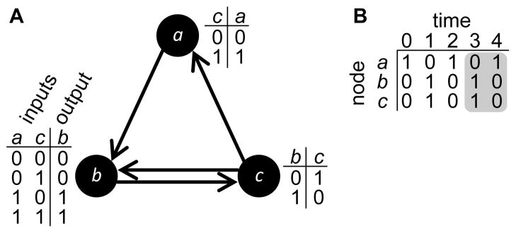
A Boolean Network example. (A) This Boolean network is composed of 3 nodes and 4 directed edges. Each node possesses a look-up table with the signal-integration logic that determines the dynamics of the Boolean network by defining the expression state of the node at time t + 1 as a function of the states of its inputs at time t. For example, the signal-integration logic for node b shows how each possible combination of expression states σ_a(t) and σ_c(t) of the inputs at time t dictate the expression state σ_b(t + 1). (B) Starting with initial states at t = 0, the states are updated according to the signal-integration logic until they repeat, forming an attractor (shaded region), which is analogous to a phenotype. In this example, the attractor length is two. For visual clarity, the size of the network depicted here is much smaller than those used in this study.

$${\sigma }_i(t+1)=f_i({\sigma }_{i_1}(t),\dots ,{\sigma }_{i_{k_{\text{in},i}}}(t)),$$ (1)

where σ_i1, …, σ_ikin,iare the states of the k_in,i regulators of node i. This process is deterministic, such that the combination of the states of all N nodes Σ_t = σ₁(t), …, σ_N (t) at time t, referred to as a configuration, will always result in the same updated configuration Σ_t+1. Since the number of possible configurations is finite (2^N), this deterministic updating of node states will eventually lead to a previously encountered configuration. Specifically, given an initial configuration Σ₀, there is some time t+l in which the previously encountered configuration Σ_t is encountered again:

$${\mathrm{\sum }}_0\to \cdots \to {\mathrm{\sum }}_t\to \cdots \to {\mathrm{\sum }}_{t+l-1}\to {\mathrm{\sum }}_t\to \cdots .$$ (2)

Such a cycle P_∞(Σ₀) is referred to as an attractor of length l,

$$P_{\infty }({\mathrm{\sum }}_0)={\mathrm{\sum }}_t\to \cdots \to {\mathrm{\sum }}_{t+l-1},$$ (3)

which we consider as a phenotype and which has been likened to cell fate (Huang et al., 2005). For any given GRN, we refer to the collection of all its unique attractors as the attractor set Ω, and the number of its unique attractors |Ω| as the cardinality of the attractor set.

Though abstract, Boolean networks have been successfully used to predict gene expression in multiple model systems, including the yeast S. cerevisiae (Serra et al., 2004), the fly Drosophila melanogaster (Albert and Othmer, 2003), and the plant Arabidopsis thaliana (Espinosa-Soto et al., 2004). GRNs modeled using Boolean networks can be perturbed in explicitly defined ways, and the resulting attractors of large ensembles of GRNs are easily identified and compared. Therefore, this model system is a valuable tool with which to address questions about the robustness and evolvability of GRNs (Aldana et al., 2007; Payne and Moore, 2011; Pechenick et al., 2012).

2.2. Degree distribution

GRNs with heavy-tailed output degree distributions were generated by approximating a power-law distribution, as follows. For each node in the GRN, its number of regulatory targets k_out was selected from the distribution (Darabos et al., 2009):

$$p(k_{\text{out}})=\frac{1}{Z(\gamma )}{k}_{\text{out}}^{-\gamma },$$ (4)

with the normalization constant $Z(\gamma )={\sum }_{j=1}^N{j}^{-\gamma }$. Drawing the output degrees from this distribution and then randomly selecting k_out regulatory targets for each node resulted in a network with a Poisson input degree distribution. The combination of Poisson input and power-law output degree distribution was chosen because it more closely resembles experimental regulatory network data from E. Coli, B. Subtilis, and S. cerevisiae than the degree distributions of homogeneous random topologies (Aldana et al., 2007).

2.3. Assortativity

Degree assortativity r ∈ [−1, 1] is a global network property that captures the extent to which nodes of similar degree are connected to one another (Newman, 2002). It is calculated as the following coefficient:

$$r=\frac{\frac{1}{M}{\sum }_i{j}_i{k}_i-{(\frac{1}{M}{\sum }_i\frac{1}{2}(j_i+k_i))}^2}{\frac{1}{M}{\sum }_i\frac{1}{2}(j_i^2+k_i^2)-{(\frac{1}{M}{\sum }_i\frac{1}{2}(j_i+k_i))}^2},$$ (5)

where j_i, k_i are the degrees of the nodes at the ends of edge i, and M is the number of edges in the network. When r > 0 the network is said to be assortative or positively assortative, and when r < 0 it is disassortative or negatively assortative. GRNs are directed networks, and as such j and k can either represent the in- or out-degree, thereby resulting in four different ways to perform the above calculation (Foster et al., 2010). Following our earlier work (Pechenick et al., 2012), we focus exclusively on the case where both j and k are out-degrees, and will refer to this out-out assortativity (Foster et al., 2010) simply as assortativity.

We used an iterative edge-swapping method to rewire each GRN to achieve the desired assortativity value (Milo et al., 2003; Payne and Eppstein, 2009). Briefly, two edges i → j and x → y were randomly chosen for an edge-swap that resulted in two new edges i → y and x → j. The assortativity of the GRN with the new edges was compared to the original GRN, and if the edge-swap altered the value in the desired direction the new edges were kept. Otherwise, the new edges were reverted to the original edges. This process was repeated until the desired value was reached, or a maximum number of swaps was attempted (Section 2.6). This method preserves the degree distribution of the GRN, which enables an investigation of the effects of assortativity on a GRN while controlling for the effects of its degree distribution.

2.4. Gene birth, conservation, and innovation

Our method for simulating gene birth follows the duplication and divergence procedure of Aldana et al. (2007) and is outlined in Fig. 2. A node c is selected at random for duplication and is included in the new GRN as node d. The divergence of d from c is accomplished in four steps: (1) outgoing edges are rewired such that they point to randomly chosen nodes (preserving the out-degree of d), (2) incoming edges are rewired such that they emanate from randomly chosen nodes (preserving the in-degree of d), (3) the signal-integration logic of d is randomly initialized such that each entry is filled with a 0 or 1 with equal probability (ρ = 0.5), and (4) the signal-integration logic of the regulatory targets of d are expanded. Upon expansion, the regulatory targets of d maintain their signal-integration logic for the case where d is repressed. For the case where d is activated, the corresponding elements of signal-integration logic are assigned at random, such that each entry is filled with a 0 or 1 with equal probability. While this method is inspired by gene duplication (Aldana et al., 2007), the immediate and extreme nature of the subsequent divergence leaves no resemblance between the original gene and its duplicate. As such, the method can just as easily be thought to simulate de novo origination.

Figure 2.

Gene birth. (A) The original GRN. (B) A node c from the original GRN is duplicated to form d. Edges characterizing the relationship between c and other nodes are reproduced for d, shown with dashed arrows. (C) Edges for d are randomly rewired, preserving in- and out-degree. (D) The original GRN, now shown with signal-integration logic. (E) New signal-integration logic must be assigned for the new node and its regulatory targets in the perturbed GRN. Nodes that are not regulatory targets of d retain their original signal-integration logic (e.g., node b). Nodes a and c are regulatory targets of d, and their signal-integration logic must be expanded to account for the possibility of d being activated or repressed. The original signal-integration logic is maintained for the case where d is repressed, and new signal-integration logic is randomly chosen (ρ = 0.5) for the case where d is activated (bold). Finally, signal-integration logic is randomly chosen (ρ = 0.5) for d itself.

We are here concerned with the robustness of GRNs to gene birth, which is ascertained through a measure of conservation (Aldana et al., 2007). An attractor is considered conserved if it exists unaltered in the attractor set of the perturbed GRN. Let P_∞(Σ₀) denote the attractor of a GRN prior to gene birth, where Σ₀ is an initial configuration within the attractor itself (i.e., Σ₀ ∈ P_∞(Σ₀)). Then, let $P_{\infty }^{\prime }({\overline{\mathrm{\sum }}}_0^0)$ denote the corresponding attractor of the GRN after gene birth given the expanded initial configuration ${\overline{\mathrm{\sum }}}_0^0=\{{\mathrm{\sum }}_0,{\sigma }_{N+1}(0)=0\}$ that is identical to Σ₀ save the addition of the state of the new node, which is repressed (as indicated by the subscript). Analogously, let $P_{\infty }^{\prime }({\overline{\mathrm{\sum }}}_0^1)$ denote the attractor where the new node is activated in the initial configuration ( ${\overline{\mathrm{\sum }}}_0^1=\{{\mathrm{\sum }}_0,{\sigma }_{N+1}(0)=1\}$). In general, we use Σ̄₀ to represent an initial configuration with N + 1 nodes. Given these definitions, attractor conservation occurs when P_∞(Σ₀) is equal to either $P_{\infty }^{\prime }({\overline{\mathrm{\sum }}}_0^0)$ or $P_{\infty }^{\prime }({\overline{\mathrm{\sum }}}_0^1)$. To compare attractors of different dimension, the state of the new node σ_N+1 is ignored (Aldana et al., 2007). A GRN demonstrates set conservation if every attractor in the GRN prior to gene birth is conserved after gene birth.

We are additionally concerned with the evolvability of GRNs upon gene birth, which is ascertained through a stringent measure of innovation (Aldana et al., 2007). Innovation is said to have occurred if at least one novel attractor exists after gene birth. This measure is stringent because an attractor $P_{\infty }^{\prime }({\overline{\mathrm{\sum }}}_0)$ is only considered novel if there is no overlap between its configurations and those of the attractors in the attractor set prior to gene birth. Formally, an attractor $P_{\infty }^{\prime }({\overline{\mathrm{\sum }}}_0)$ is novel if $\forall {\overline{\mathrm{\sum }}}_t\in P_{\infty }^{\prime }({\overline{\mathrm{\sum }}}_0)\nexists {\overline{\mathrm{\sum }}}_t\in P_{\infty }({\mathrm{\sum }}_0)\forall P_{\infty }({\mathrm{\sum }}_0)\in \mathrm{\Omega }$.

2.5. Out-components

The regulatory influence of node i is reflected in its out-component (OC), which is the set of weakly connected nodes in a directed network that is reachable via directed paths staring from i (Figure 3). Therefore, the OC of node i is the set of all nodes that i may directly or indirectly influence. The OC of node i was determined by identifying all regulatory targets of node i, all of their regulatory targets, and so on until every reachable node was identified. Regulatory targets were identified strictly on a topological basis, where j is a regulatory target of i as long as the edge i → j exists in the network. Mean OC size (S̄) for a GRN was calculated as follows:

$$\overline{S}=\frac{{\sum }_{i=1}^N{S}_i}{N},$$ (6)

where S_i is the number of nodes in the OC of node i.

Figure 3.

Out-components of GRNs. An out-component (OC) can be drawn around each node in the GRN. The OC of node i consists of six nodes (large shaded region), and the OC of node j consists of three nodes (small shaded region). There are two nodes that belong to the OCs of both i and j (overlap of shaded regions).

2.6. Simulation details

Weakly connected GRNs without self-loops were generated for size N = 30. This size was selected as a compromise between those GRNs that are large enough to achieve a range of assortativity values, but also small enough to compute the numerous simulations described below. In particular, the lengths of individual attractors produced by chaotic GRNs grow very quickly as N is increased (Kauffman, 1993), and some of these attractors may be effectively too long to enumerate. Therefore the ability to calculate even modest numbers of attractors is limited by the choice of N.

Although the dynamics of biological GRNs are influenced by their autoregulatory self-loops (Alon, 2006), their presence is confounding with respect to understanding the effects of assortativity. Increasing the number of self-loops is a trivial way to increase the assortativity of a network, as by definition a self-loop connects a node to itself, and thus always contributes positively to assortativity. Self-loops were therefore excluded from the main analysis in order to isolate the effects of assortativity from those of self-loops.

Multiple heavy-tailed degree distributions were generated by drawing out-degrees from power-law distributions with γ = 3.10, 2.25, 1.81, 1.55. These values of γ were chosen because they yield distributions such that k̄_in = 1.3, 2, 3, 4, respectively. These k̄_in were calculated for the specific size of the GRNs considered in this study (Aldana et al., 2007):

$${\overline{k}}_{\text{in}}=\frac{{\sum }_{j=1}^N{j}^{1-\gamma }}{{\sum }_{j=1}^N{j}^{-\gamma }}$$ (7)

(k̄_in = 1.3 was chosen because k̄_in = 1 only exists in the limit of γ → ∞). Note that k̄_in = k̄_out.

Boolean networks lie in one of three dynamical regimes: ordered, critical, or chaotic. The sensitivity of these GRNs to perturbation defines their dynamical regime, and can be calculated as s = 2ρ(1 − ρ)k̄_in, where ρ is the probability of assigning a 1 within the signal-integration logic of the GRN. A GRN is in the chaotic regime when s > 1, the ordered regime when s < 1, and the critical regime when s = 1 (Shmulevich and Kauffman, 2004). We use ρ = 0.5 across all simulations, and the above k̄_in values thus yield the desired dynamical regimes (Table 1). Visual inspection of Derrida plots (Derrida and Pomeau, 1986) confirmed that the selected parameters for each degree distribution produced GRNs in the respective regimes (Fig. S1). After the topology of a GRN was created, the signal-integration logic of each node was generated at random, such that the probability of choosing a 0 or 1 was equal.

Table 1.

Lower and upper bounds on assortativity.

Regime	γ	k̄out	Assortativity (r ± 0.01) Bounds
Ordered	3.10	1.3	−0.29 ≤ r ≤ 0.48
Critical	2.25	2.0	−0.49 ≤ r ≤ 0.20
Chaotic	1.81	3.0	−0.58 ≤ r ≤ 0.01
	1.55	4.0	−0.64 ≤ r ≤ −0.02

For each of the four values of k̄_out, 45000 GRNs were generated with assortativity values that lie within the bounds shown in Table 1. While the theoretical bounds of assortativity are r ∈ [−1, 1], in practice they are constrained by degree distribution (Dodds and Payne, 2009; Johnson et al., 2010). The bounds used here were experimentally determined for each k̄_out by performing first 2000 edge-swaps toward an assortativity value of −1, and then for the same GRN another 2000 edge-swaps toward a value of 1 on each of 1000 GRNs. This number of edge-swaps was chosen as a balance between computational efficiency and achieving a wide range of assortativity values (Pechenick et al., 2012). From each resulting distribution of assortativity ranges, a representative range was chosen such that both low and high bounds were together contained within 25% of observed ranges.

It is important to point out that sampling from a degree distribution yields a specific degree sequence, which may vary between successive draws from the distribution. To ensure that each degree sequence was represented at each assortativity value, we adopted the following experimental design. Within each set of assortativity bounds, 9 linearly spaced assortativity values were chosen, and 5000 degree sequences were tuned to within 0.01 of every value, preserving weak-connectivity and prohibiting self-loops. Thus each of the 5000 degree sequences are represented at every one of the 9 assortativity values. For each of the 5000 degree sequences, the same signal-integration logic was assigned and the same gene birth event was performed at every assortativity value. As a result of this approach, assortativity was the sole property varied for each degree sequence.

As with assortativity bounds, the null distribution of assortativity values for a particular GRN depends on k̄_out (Foster et al., 2010; Johnson et al., 2010). To calculate these null distributions, 1000 GRNs were constructed for each k̄_out without regard to assortativity. To remove any potential structural bias introduced during construction, 10 × M random edge-swaps were performed for each GRN, such that degree sequence, weak connectivity, and lack of self-loops were all preserved (Maslov and Sneppen, 2002). Assortativity was then measured for each GRN, and these 1000 assortativity values served as a null distribution for each k̄_out. The null distributions were used to verify that the bounds of assortativity considered in this study (Table 1) lie outside what is expected at random.

To calculate conservation and innovation, it is necessary to characterize the entire attractor set of the GRNs both before and after gene birth. While such exhaustive enumeration is possible for small GRNs (Aldana et al., 2007; Payne and Moore, 2011), the size of the GRNs considered herein necessitated a sampling approach. For each GRN, both before and after gene birth, we randomly sampled 10⁶ initial configurations Σ₀, recorded the corresponding attractors, and compared the attractor sets of the perturbed and original GRNs. To ensure the accuracy of our conservation measure, we additionally took a single configuration from each attractor of the original GRN and used it as an initial configuration in the perturbed GRN. We then recorded the attractors of the perturbed GRN for the case where the new node was active and for the case where it was repressed. This ensured that any attractor present in both the original and perturbed GRNs would not be overlooked as a result of undersampling. Analogously, we used every configuration in the attractor set of the perturbed GRN as an initial configuration in the original GRN, recorded the corresponding attractors, and updated the attractor set if necessary. This allowed us to ensure the accuracy of our innovation measure by determining whether novel attractors were in fact novel or were simply overlooked in the original GRN as a result of undersampling. These two post-sampling steps were repeated until no new attractors were discovered in either the original or perturbed GRNs.

3. Results

3.1. The influence of assortativity on conservation and innovation

The sensitivity of conservation and innovation to changes in assortativity varied between dynamical regimes (Fig. 4). Conservation decreased slightly with assortativity in the ordered regime (Fig. 4a), but increased in the critical (Fig. 4b) and chaotic regimes (Fig. 4c–d). The extent of this increase became more pronounced as the dynamical regime of the GRN shifted toward chaos. For example, when k̄_out = 4, we observed a 116% increase in conservation when comparing the GRNs of the lowest and highest assortativity values. Innovation decreased with assortativity in the critical (Fig. 4b) and chaotic regimes (Fig. 4c–d), and this trend again became more pronounced as the GRNs became more chaotic. In contrast, no trend was observed between innovation and assortativity in the ordered regime (Fig. 4a). These results corroborate previous observations (Aldana et al., 2007) that the dynamical regime of a GRN impacts its capacity for conservation and innovation, and highlights the sensitivity of these properties to changes in assortativity. Furthermore, we observed that assortativity does not influence the dynamical regime of a GRN (Fig. S1), which underscores that any sensitivity to assortativity is not simply a byproduct of variation within or between dynamical regimes.

Figure 4.

Proportion of GRNs with set conservation, innovation, or both as a function of assortativity. (Above) Light gray bars show the proportion of GRNs at a fixed assortativity value that exhibited set conservation after gene birth. Medium gray bars represent the proportion that exhibited innovation. Dark gray bars show the overlap, which is the proportion that both conserved and innovated. These overlap proportions are mirrored above and below the x-axis such that heights of light gray and medium gray bars accurately portray total conservation and innovation, respectively. Each bar is a proportion of 5000 GRNs for each of: k̄_out ∈ {1.3, 2.0, 3.0, 4.0} (denoted by A–D) and 9 assortativity values. Each degree sequence and gene birth combination is represented at every assortativity value. (Below) The proportion of the overlap is shown at a zoomed-in scale. Note that the domains for assortativity differ for A–D (Table 1). Note also that total proportions of conservation and innovation may not add up to 1, as some GRNs may exhibit neither. The legend in (D) applies to all panels. The percentage change from the smallest to the largest assortativity value is shown for conservation, innovation, and both. Statistical significance for Spearman’s correlation is denoted by * (p < 0.05), ** (p < 0.01), or *** (p < 0.001). Vertical dashed lines show the minimum and maximum assortativity values for the middle 95% of the null distribution for each k̄_out (see Section 2.6).

Following gene birth, some GRNs exhibited conservation and innovation simultaneously (Fig. 4). In the ordered regime, the proportion of networks able to achieve this balance decreased slightly as assortativity increased (Fig. 4a), while in the critical regime no trend was observed (Fig. 4b). In the chaotic regime, this proportion increased dramatically. For instance, when k̄_out = 4, the proportion of networks exhibiting both conservation and innovation increased by 176%, when comparing the GRNs with the lowest and highest assortativity values.

In a similar but separate analysis, GRNs with self-loops displayed qualitatively similar results as GRNs without self-loops (Fig. S2). Specifically, ordered (Fig. S2a) and critical (Fig. S2b) GRNs with self-loops were minimally affected by assortativity, whereas chaotic GRNs with self-loops exhibited increases in conservation and decreases in innovation (Fig. S2c–d). Furthermore, these latter trends produced concomitant increases in the proportion of GRNs that exhibited both conservation and innovation, e.g., for GRNs with k̄_out = 4 where this proportion increased 173% from the lowest to highest assortativity value (Fig. S2d). And, while a significant increase was not observed for GRNs with k̄_out = 3 when considering all assortativity values (Fig. S2c), upon considering the highest 7 assortativity values there was a significant increase of 61% (Spearman’s correlation, p < 0.01) in GRNs that both conserved and innovated.

In contrast to GRNs without self-loops, critical GRNs with self-loops appeared to be less sensitive to the effects of assortativity (Fig. S2a), whereas ordered GRNs with self-loops displayed an increased rate of innovation along with an apparent lack of trend in those GRNs that both conserved and innovated (Fig. S2b). While these differences may point to an interaction between the effects of assortativity and self-loops, elucidating such a mechanism is beyond the scope of the current investigation.

Qualitative changes in conservation and innovation between dynamical regimes and multiple assortativity values were also observed for larger GRNs where N = 100 (Fig. S3). Ordered (Fig. S3a) and critical (Fig. S3b) GRNs with N = 100 were relatively insensitive to changes in assortativity, whereas for chaotic GRNs with N = 100 (Fig. S3c–d) increasing assortativity produced increased conservation and decreased innovation. And, while GRNs that both conserved and innovated were too few to detect statistically significant trends, the chaotic GRNs with high assortativity values were seemingly more likely to both conserve and innovate compared with their counterparts with lower assortativity values (Fig. S3c–d). Unfortunately, the power to study the effects of assortativity on GRNs with N = 100 is substantially limited by the small numbers of GRNs capable of simultaneous conservation and innovation (irrespective of N), along with the computational difficulties of calculating the long attractors in Boolean networks of this size (particularly in the chaotic regime). Therefore, in the following sections we focus on GRNs with N = 30 and without self-loops, explaining the increase in conservation and decrease in innovation observed in critical (Fig. 4b) and chaotic (Fig. 4c–d) GRNs, along with the slight decrease in conservation observed in ordered (Fig. 4a) GRNs.

3.2. The influence of assortativity on the cardinality of the attractor set

Conservation requires that a GRN maintains all of the attractors in its attractor set after gene birth. In Fig. 5, we depict the relationship between the cardinality of the attractor set and assortativity. We observe a slight increase in the cardinality of the attractor set for ordered GRNs (Fig. 5a, statistically significant but not visually discernable) and a strong decrease for critical and chaotic GRNs (Fig. 5b–d). Since it is easier to conserve fewer attractors than many (Fig. S4), one simple way in which assortativity influences conservation is by modifying the cardinality of the attractor set. This explains, at least in part, the negative trend between conservation and assortativity in ordered GRNs, and the corresponding positive trends in critical and chaotic GRNs (Fig. 4).

Figure 5.

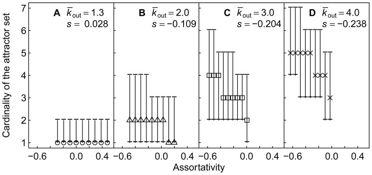
Cardinality of the attractor set as a function of assortativity. Points represent the median cardinality of the attractor set before gene birth in 5000 GRNs at a fixed assortativity value, whereas error bars represent the 25^th and 75^th percentiles. GRNs are grouped according to their k̄_out and assortativity value, as in Figure 4. For all k̄_out, the cardinality of the attractor set is significantly affected by assortativity (Spearman’s correlation coefficient (s), p ≪ 0.001).

3.3. The influence of assortativity on the conservation of individual attractors

In addition to influencing the cardinality of the attractor set, assortativity may separately impact the probability with which individual attractors are conserved. To determine the likelihood of conserving an individual attractor irrespective of the number of attractors in the attractor set, we measured the proportion of all attractors from all GRNs that were conserved after gene birth (Fig. 6; note that this proportion is different from that of Fig. 4, which depicted the proportion of GRNs that exhibited set conservation.) Further, we split this proportion into two categories: (1) the trivial case resulting from the constitutive repression of the new node within the attractor, and (2) a nontrivial case where an attractor was conserved despite activation of the new node within the attractor. For GRNs in the ordered regime, we observed no relationship between assortativity and the conservation of individual attractors (Fig. 6a). In contrast, the conservation of individual attractors increased significantly for GRNs in the critical and chaotic regimes (Fig. 6b–d), for both of the aforementioned categories. Therefore, the attractor sets of assortative GRNs are not only easier to conserve because of their reduced cardinality (Fig. 5), but also because their constituent attractors are themselves easier to conserve.

Figure 6.

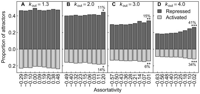
Proportion of attractors that are conserved after gene birth as a function of assortativity. (Dark gray) Proportion of attractors that are conserved as a result of the repression of the new node in all of the configurations in the attractor. (Light gray) Proportion of attractors that are conserved despite the new node being activated. For each bar, all attractors are considered for 5000 GRNs with the same k̄_out and a fixed assortativity value, as described in Figure 4. Note that the domains for assortativity differ for A–D. The legend in (D) applies to all panels. The percentage change from the smallest to the largest assortativity value is shown for each form of attractor conservation. Statistical significance for Spearman’s correlation is denoted by * (p < 0.05), ** (p < 0.01), or *** (p < 0.001).

3.4. The influence of attractor length on the conservation of individual attractors

Why are the individual attractors of assortative GRNs easier to conserve? We have shown elsewhere that increased assortativity leads to a decrease in attractor length (recapitulated here in Fig. S5), and that shorter attractors are more phenotypically robust (Pechenick et al., 2012). In Fig. 7, we show the relationship between the lengths of attractors that were or were not conserved as a function of assortativity. The lengths of conserved attractors tended to be shorter than those of non-conserved attractors, suggesting that individual attractors of assortative GRNs are easier to conserve because they are shorter.

Figure 7.

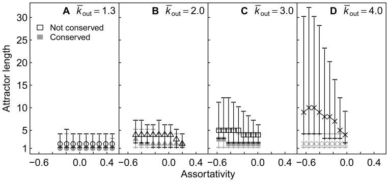
Lengths of attractors that were or were not conserved as a function of assortativity. Each point represents the median length of unique attractors before gene birth in 5000 GRNs at a fixed assortativity value. Error bars represent the 25^th and 75^th percentiles. Medians and percentiles for attractors that were not conserved are shown in black, whereas those for attractors that were conserved are shown in gray. GRNs are grouped according to their k̄_out and assortativity value, as in Figure 4. Conserved attractors are significantly shorter for every assortativity value and every k̄_out (Wilcoxon Rank Sum test, p ≪ 0.001).

In order to more completely address the role of attractor length on attractor conservation, we examined its influence on the dynamics of (1) the new node and (2) the regulatory targets of the new node. We observed that shorter attractors had a reduced probability of activating the new node, relative to longer attractors (Fig. S6). Since attractor conservation is certain when the new node is repressed, shorter attractors are expected to be conserved with higher likelihood than longer attractors.

When the new node is activated, attractor conservation is no longer certain. To describe how attractors may be conserved in this case, we introduce the term target rule utilization (U), which is defined as the number of elements in the expanded (see Section 2.4) signal-integration logic of all the regulatory targets of the new node that are accessed at some point during the attractor. The variable U thus captures the number of unique binary decisions encountered within the attractor as a direct result of the new node being activated. In other words, it is the extent to which the new node is capable of perturbing that specific attractor. This is evident in the relationship we observed between the probability of attractor conservation, p(C), and U, where $p(C)={(\frac{1}{2})}^U$ (Fig. 8). This simple relationship can be understood as follows: With each increase of U by 1, the GRN must access an additional element of the signal-integration logic that never existed in the GRN prior to gene birth. And with each novel element, there is a 50% chance that the expression of the regulatory target will deviate from what it would have been in the original GRN (since ρ = 0.5, see Section 2.4). Such a deviation changes the attractor, preventing its conservation. Thus, the likelihood of conservation is the combined probability that none of the U accessed elements cause a deviation.

Figure 8.

Proportion of attractors that are conserved after gene birth (p(C)) as a function of target rule utilization (U). The points are observed proportions of all attractors for 45000 GRNs for each value of k̄_out across all measured assortativity values, and data that exists for larger values of U are not shown if there is no conservation. The predicted proportion of conservation is shown by the solid line.

Since U considers the influence of a new node over all its regulatory targets, one explanation for how some GRNs could produce attractors with higher values of U is that the new node simply has more regulatory targets. However, this cannot explain the observed differences in attractor conservation, because we ensured that the same new nodes with their respective out-degrees were tested at every different assortativity value within a dynamical regime (see Section 2.6).

Another possibility is that U is influenced by the length of the attractor under consideration. Here, the intuition is that an attractor that is short realizes only a few combinations of the regulatory inputs in its signal-integration logic, and this is likely to result in a small value of U. In contrast, a long attractor that realizes many combinations may be more likely to encounter more of those specific combinations that occur as a result of activation of the new node, resulting in a higher value of U. In support of this hypothesis, we observed that the average value of U increased with increasing attractor length (Fig. S7). And, since shorter attractors produce a smaller average U (Fig. S7), they are expected to be conserved more often than longer attractors.

3.5. The influence of out-components (OCs) on innovation

Innovation was also sensitive to the effects of assortativity, but unlike conservation the trends were generally decreasing (Fig. 4b–d). It was apparent that innovation was more likely when the new node regulated many targets (Fig. S8), which suggested that the extent of the regulatory influence exerted by the new node impacted the likelihood of innovation. However, our experimental approach ensured that there was the same distribution of new node out-degrees present for GRNs at every assortativity value (Section 2.6), thus requiring an additional explanation for how the extent of the regulatory influence could change with assortativity.

The out-component (OC) of a node in a GRN is characterized by the nodes that it potentially regulates (Fig. 3), and we reasoned that the new node might exert a different amount of regulatory influence depending on whether its OC was large or small. The mean OC size of a GRN shrinks as assortativity increases (Fig. S9), and might therefore explain how assortativity influences innovation.

To examine the effects of OCs on innovation, we considered only the most assortative GRNs, which have the smallest mean OC sizes yet still exhibit some variation in OC sizes (Fig. S9). This approach allowed us to establish the independent effect of OC size. We then grouped networks by the out-degree of the new node and whether its OC was large or small (Figure 9). We observed that for GRNs where the new node has many regulatory targets, innovation does not depend on the OC size of the new node. This suggests that a new node with high out-degree exerts enough of an influence over the GRN that the size of its OC matters less. In contrast, for GRNs with new nodes that possess fewer regulatory targets, innovation was sensitive to the OC size of the new node, such that a new node with a small OC was less likely to innovate than a new node with a large OC. This underscores that innovation is sensitive to the regulatory influence of the new node, and also that the extent of this influence is shaped by more than simply the number of targets regulated. Since GRNs that follow a heavy-tailed out-degree distribution are likely to have new nodes with low out-degree, the observed effect is expected to be wide-reaching despite not being statistically significant for higher out-degree. Therefore, as assortative GRNs possess smaller OCs (Fig. S9), they are expected to show reduced rates of innovation (Fig. 4).

Figure 9.

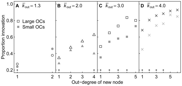
Proportion of innovation as a function of the out-degree of the new node and whether the new node possesses a large or small out-component (OC). The 5000 GRNs at the highest assortativity value for each k̄_out were binned by the out-degree of the new node. Each out-degree bin was then split into two groups according to whether the new node possesses a large OC (larger or equal to the median OC size) or small OC (smaller than the median OC size). Black markers represent the proportion of GRNs that innovated at least one attractor where new nodes possess large OCs, and gray markers represent innovation for GRNs where new nodes possess small OCs. Asterisks mark significant differences in proportions between large and small OC categories (p < 0.05, Pearson’s chi-squared test). Only out-degrees for which at least 30 GRNs were present in large and small OC bins are plotted.

4. Discussion

Two central forces driving the evolution of GRNs are gene duplication (Lynch and Conery, 2000) and de novo origination (Carvunis et al., 2012). Using a computational model of genetic regulation, we have shown that the conservation of existing phenotypes by GRNs subject to gene birth is influenced by assortativity. To explain this observation, we have proposed the following pair of mechanisms. First, the cardinality of the attractor set shrinks with increasing assortativity, thereby making set conservation more likely. Attractor set cardinality is akin to the number of potential cell types that may be reached via differentiation (Huang et al., 2009), and a cell with an assortative GRN might thus have a reduced capacity for differentiation. As GRNs grow in size and complexity, the cardinality of the attractor set also grows (Kauffman, 1971), making it unlikely that all possible attractors would represent normal cell types (Huang et al., 2009). In this case, an assortative GRN would limit the number of normally unaccessed attractors, some of which may correspond to an abnormal phenotype. To our knowledge, this is the first study to identify a relationship between the assortativity of a GRN and the cardinality of its attractor set.

Second, attractor length shrinks with increasing assortativity, and shorter attractors are more likely to be conserved. This is consistent with previous observations regarding the robustness of shorter attractors (Luo and Turner, 2011). A number of theoretical studies have shown a correlation between attractor length and mutational robustness, where GRNs with shorter attractors were more robust to genetic perturbation (Mihaljev and Drossel, 2009; Szejka and Drossel, 2010). And, we have previously shown that GRNs with shorter attractors are more phenotypically robust when faced with mutation to their cis-regulatory logic (Pechenick et al., 2012). In line with these previous observations, we have now shown that shorter attractors are also less likely to be affected by gene birth, because their small sizes limit the extent to which novel regulatory decisions are encountered within the context of the existing regulatory program. Therefore, assortative GRNs with their shorter attractors are robust to a variety of genetic perturbations.

In contrast to conservation, we found that the likelihood of innovation by a GRN decreased with increasing assortativity. This was due to a shrinking average sphere-of-influence associated with increased assortativity. Specifically, the out-component (OC) of the new node was on average smaller for assortative GRNs, and thus the regulatory influence of the new node was lessened. This is related to our previous observation that in-components (ICs) tend to shrink with increasing assortativity (Pechenick et al., 2012). The capacity for a new gene to yield an innovation is thus tied to its regulatory influence; however, such innovation is typically deleterious in natural systems (Lynch and Conery, 2000). Indeed, it has been shown that gene duplication events in S. cerevisiae were less likely to occur in well connected portions of the protein-protein interaction network (Li et al., 2006). Thus with their smaller OCs, assortative GRNs may to some extent be shielded from perturbation, and less likely to utilize these perturbations for innovation.

The relationship between GRN components and robustness has also recently been investigated by Peixoto (2012), who observed that populations of GRNs evolved under strong selection for environmental robustness tended to develop small, dense subgraphs. These subgraphs acted as master regulators that were segregated from much of the GRN, and were therefore largely autonomous. The robustness of GRNs to environmental perturbation is related to their robustness to genetic perturbation (Ciliberti et al., 2007b), and the reported relationship between dense subgraphs and robustness is consistent with our own observations. We previously linked small, autonomous ICs to high phenotypic robustness in the face of mutation to the cis-regulatory logic of the GRN (Pechenick et al., 2012), and we here show that small OCs limit the extent of the perturbation caused by gene birth. Taken together, these studies illustrate complementary processes by which GRNs might achieve higher robustness. Peixoto (2012) allowed the transition from a random topology to a segregated core topology through changes in the degree distribution, and we showed that changing the assortativity while holding the degree distribution constant can lead to changes in ICs (Pechenick et al., 2012) and OCs. Therefore, there may exist multiple avenues of structural alteration for an evolutionary process to achieve a GRN with a highly robust topology.

We further observed that increasingly assortative GRNs were more likely to simultaneously conserve and innovate. Assortative GRNs displayed a marked increase in conservation that outpaced the decrease in innovation, with the result that assortative GRNs more often achieved both. Thus, an apparent tradeoff of assortative GRNs–that they are highly robust but less evolvable–is not the whole story. Instead, we found that assortative GRNs maximize the intersection of robustness and evolvability. While innovation is rarely tolerated in natural systems (Lynch and Conery, 2000), it will sometimes produce a phenotype on which selection can act (Levine and Tjian, 2003), and our results suggest that assortative GRNs may be poised for the exploration of novel phenotypes conditional upon the conservation of existing phenotypes.

The influence of assortativity on the overlap of robustness and evolvability varied with dynamical regime. Ordered and critical GRNs showed a weak negative trend and no trend, respectively, whereas chaotic GRNs showed positive trends. This is consistent with our previous observations, where the phenotypic robustness of ordered and critical GRNs were relatively insensitive to changes in assortativity (Pechenick et al., 2012). This relative insensitivity of critical GRNs is noteworthy, as there is some evidence to support the hypothesis that biological regulatory networks operate close to criticality (Shmulevich et al., 2005; Nykter et al., 2008). However, the differences in trends highlight a consequence of analyzing populations of GRNs without considering assortativity. For example, Aldana et al. (2007) observed that critical GRNs jointly conserve and innovate more often than ordered or chaotic GRNs, and cited this as further support for the criticality hypothesis. Yet, once GRNs are subdivided by their assortativity, we saw that assortative chaotic (k̄_out = 3.0) GRNs maximized this overlap of robustness and evolvability. Remarkably, the assortativity of a GRN had no impact on its dynamical regime, and therefore the observed high overlap for assortative chaotic GRNs was not the result of their transitioning toward criticality. In a separate study, Payne and Moore (2011) performed an exhaustive analysis of the robustness of signal-integration logic in small regulatory circuits, and also observed that chaotic GRNs can maximize these two properties. Taken together, these results present a challenge to the current understanding of how criticality provides an evolutionary advantage over GRNs that operate in the chaotic dynamical regime.

One limitation of this study is a lack of consideration of selection and the potential fitness effects of innovation. While gene duplicates are thought to initially experience relaxed selection, many eventually fall under strong purifying selection (Wagner, 2002), and it is this selection that produces innovation from variation (Wagner, 2008). We have shown that assortativity influences the likelihood that a GRN produces variation in the form of new phenotypes, but does assortativity affect the evolution of a specific phenotype with improved fitness? This question can be addressed through the in silico evolution of GRNs that are under selection for specific phenotypes that confer a fitness advantage (Oikonomou and Cluzel, 2006; Greenbury et al., 2010). Using such an approach, it has been observed that topological properties of GRNs, such as degree distribution, affect their ability to evolve specific phenotypes (Oikonomou and Cluzel, 2006; Greenbury et al., 2010), and future studies should examine whether and how assortativity plays a role.

Another direction of future research concerns the robustness of GRNs to recombination. Recombination is a major force that generates genetic variation, and the robustness of GRNs to recombination is therefore of considerable interest (Martin and Wagner, 2009). Through computational analysis of an alternative model of GRNs, Martin and Wagner (2009) showed that populations of GRNs are more robust to genetic point mutations after evolving to recombination-selection balance. However, the effects of nonrandom assortativity were not considered. Therefore, a natural extension of this work will be to assess the influence of assortativity on the robustness of GRNs to recombination.

Our theoretical work has suggested that the assortativity of a GRN influences its robustness and evolvability, and experimental evidence will be instrumental in determining the biological relevance of these findings. For example, future advances in synthetic biology (Purnick and Weiss, 2009) may one day enable the construction of synthetic GRNs that are large enough to directly evaluate the influence of assortativity on robustness and evolvability. In the meantime, our attention turns to the assortativity values of network representations of existing biological datasets (Piraveenan et al., 2012), and interpreting these values in the context of the underlying GRN of a cell. To understand the complex nature of this task, it is important to keep in mind the multiple layers of genetic regulation. For example, the chromatin immunoprecipitation (ChIP) data produced by ENCODE (ENCODE Project Consortium et al., 2011) may eventually lead to a comprehensive human transcription factor network. Properties of this network, such as assortativity, could be calculated, but its topology represents only a single regulatory layer of the GRN. Additional layers that could be considered include post-transcriptional regulation by microRNAs (Chen and Rajewsky, 2007) and post-translational regulation by protein phosphorylation (Linding et al., 2007, 2008). Each time a new layer of regulation is included, the topology of the apparent GRN will change, and properties such as assortativity may also change. This is one of the advantages of first taking a theoretical approach to understanding the effects of the assortativity of a GRN. Multiple layers of regulation can be implicitly represented in an abstract computational model, and this allows us to infer how functional properties of the GRN may be influenced by its topology. It will be important to place the results of future experimentation, such as the assortativity of experimental datasets and the phenotypic output of synthetic GRNs, in the appropriate context of the multiple layers of gene regulation.

Supplementary Material

01

Figure S1: Derrida plot showing the Hamming distance between two updated GRN configurations as a function of the Hamming distance between their initial configurations. For a GRN, an initial configuration Σ₀ was perturbed by randomly flipping initial states to yield Σ̃₀. H(Σ₀, Σ̃₀) represents the Hamming distance between these two initial configurations. Each configuration was then updated, resulting in two new configurations Σ₁ and Σ̃₁, respectively. H(Σ₁, Σ̃₁) is the Hamming distance between the updated configurations. This process was repeated with 1000 randomly generated Σ₀ for each possible value of H(Σ₀, Σ̃₀), and each Σ₀ was paired with randomly chosen (ρ = 0.5) signal-integration logic. The above was performed for 1000 GRNs for each k̄_out and assortativity value. The resulting 9 sets of points for each k̄_out are overlaid, and due to their similarity cannot be visually distinguished. The line y = x is shown for reference.

Figure S2: Proportion of GRNs that have self-loops with set conservation, innovation, or both as a function of assortativity. (Above) Light gray bars show the proportion of GRNs at a fixed assortativity value that exhibited set conservation after gene birth. Medium gray bars represent the proportion that exhibited innovation. Dark gray bars show the overlap, which is the proportion that both conserved and innovated. These overlap proportions are mirrored above and below the x-axis such that heights of light gray and medium gray bars accurately portray total conservation and innovation, respectively. Each bar is a proportion of 1000 GRNs for each of: k̄_out ∈ {1.3, 2.0, 3.0, 4.0} (denoted by A–D) and 9 assortativity values. Each degree sequence and gene birth combination is represented at every assortativity value. (Below) The proportion of the overlap is shown at a zoomed-in scale. Note that the domains for assortativity differ for A–D. Note also that total proportions of conservation and innovation may not add up to 1, as some GRNs may exhibit neither. The legend in (D) applies to all panels. The percentage change from the smallest to the largest assortativity value is shown for conservation, innovation, and both. Statistical significance for Spearman’s correlation is denoted by * (p < 0.05), ** (p < 0.01), or *** (p < 0.001). Vertical dashed lines show the minimum and maximum assortativity values for the middle 95% of the null distribution for each k̄_out (see Section 2.6).

Figure S3: Proportion of large GRNs (N = 100) with set conservation, innovation, or both as a function of assortativity. (Above) Light gray bars show the proportion of GRNs at a fixed assortativity value that exhibited set conservation after gene birth. Medium gray bars represent the proportion that exhibited innovation. Dark gray bars show the overlap, which is the proportion that both conserved and innovated. These overlap proportions are mirrored above and below the x-axis such that heights of light gray and medium gray bars accurately portray total conservation and innovation, respectively. Each bar is a proportion of 1800 GRNs for each of: k̄_out ∈ {1.3, 2.0, 3.0, 4.0} (denoted by A–D) and 3 assortativity values. Each degree sequence and gene birth combination is represented at every assortativity value. A total of 10³ initial configurations Σ₀ were randomly sampled for each GRN, as opposed to 10⁶ for GRNs with N = 30, as described in Section 2.6. (Below) The proportion of the overlap is shown at a zoomed-in scale. Note that the domains for assortativity differ for A–D. Note also that total proportions of conservation and innovation may not add up to 1, as some GRNs may exhibit neither. The legend in (D) applies to all panels.

Figure S4: The cardinality of the attractor set of GRNs as a function of assortativity. The data are separated into two groups: GRNs that exhibited set conservation and those that did not. Each point represents the median number of attractors before gene birth in 5000 GRNs at a fixed assortativity value. Error bars represent the 25^th and 75^th percentiles. Medians and percentiles for GRNs that did not conserve all attractors are shown in black, whereas those that did conserve are shown in gray. GRNs are grouped according to their k̄_out and assortativity value, as in Figure 4. GRNs that conserved possess significantly fewer attractors for every assortativity value and every k̄_out (Wilcoxon Rank Sum test, p < 0.01).

Figure S5: Lengths of attractors as a function of assortativity. Each point represents the median length of unique attractors before gene birth in 5000 GRNs at a fixed assortativity value. Error bars represent the 25^th and 75^th percentiles. GRNs are grouped according to their k̄_out and assortativity value, as in Figure 4. For all k̄_out, attractor lengths significantly decrease with assortativity (Spearman’s correlation, p ≪ 0.001).

Figure S6: The probability of the new node being activated in an attractor as a function of attractor length. All attractors from 45000 GRNs (before gene birth) with the same k̄_out across all measured assortativity values were binned according to their length. Points show the proportion of each bin for which at least one state in the attractor activated the new node in the network after gene birth. Only bins that contained at least 50 attractors were plotted. Note the logarithmic scale of the x-axis. For k̄_out = 3 and k̄_out = 4, the probability of activation significantly increases with attractor length (Spearman’s correlation, p ≪ 0.001).

Figure S7: Average target rule utilization as a function of attractor length. All attractors (before gene birth) were binned according to their length as in Figure S6, except only attractors with at least one state that lead to activation of the new node were considered. Target rule utilization was then averaged by the number of targets, and the mean of the bin was plotted. Only means for bins that contained at least 30 attractors were plotted. Note that x- and y-axes are presented at different scales. The p-values are presented for Spearman’s correlation.

Figure S8: Proportion of GRNs that innovated after gene birth as a function of out-degree of the new node. The points are observed proportions of all 45000 GRNs for each value of k̄_out across all measured assortativity values. Only bins that contained at least 30 GRNs were plotted. For all k̄_out, the proportion of GRNs that innovate significantly increases with out-degree of the new node (Spearman’s correlation, p < 0.05).

Figure S9: Mean out-component (OC) sizes as a function of assortativity. Each point represents the median of the distribution of mean OC sizes of 5000 GRNs (before gene birth) for a given k̄_out and fixed assortativity value. Error bars represent the 25^th and 75^th percentiles. GRNs are grouped according to their k̄_out and assortativity value, as in Figure 4. For all k̄_out, mean OC sizes significantly decrease with assortativity (p ≪ 0.001).

References

- Albert R, Othmer HG. The topology of the regulatory interactions predicts the expression pattern of the segment polarity genes in Drosophila melanogaster. Journal of Theoretical Biology. 2003;223:1–18. doi: 10.1016/s0022-5193(03)00035-3. [DOI] [PMC free article] [PubMed] [Google Scholar]
- Aldana M, Balleza E, Kauffman S, Resendiz O. Robustness and evolvability in genetic regulatory networks. Journal of Theoretical Biology. 2007;245:433–448. doi: 10.1016/j.jtbi.2006.10.027. [DOI] [PubMed] [Google Scholar]
- Aldana M, Cluzel P. A natural class of robust networks. Proceedings of the National Academy of Sciences USA. 2003;100:8710–8714. doi: 10.1073/pnas.1536783100. [DOI] [PMC free article] [PubMed] [Google Scholar]
- Alon U. An Introduction to Systems Biology: Design Principles of Biological Circuits. Chapman & Hall/CRC; 2006. [Google Scholar]
- Babu M, Luscombe N, Aravind L, Gerstein M, Teichmann S. Structure and evolution of transcriptional regulatory networks. Current Opinion in Structural Biology. 2004;14:283–291. doi: 10.1016/j.sbi.2004.05.004. [DOI] [PubMed] [Google Scholar]
- Babu MM, Teichmann SA. Evolution of transcription factors and the gene regulatory network in Escherichia coli. Nucleic Acids Research. 2003;31:1234–1244. doi: 10.1093/nar/gkg210. [DOI] [PMC free article] [PubMed] [Google Scholar]
- Carvunis AR, Rolland T, Wapinski I, Calderwood MA, Yildirim MA, Simonis N, Charloteaux B, Hidalgo CA, Barbette J, Santhanam B, Brar GA, Weissman JS, Regev A, Thierry-Mieg N, Cusick ME, Vidal M. Protogenes and de novo gene birth. Nature. 2012;487:370–374. doi: 10.1038/nature11184. [DOI] [PMC free article] [PubMed] [Google Scholar]
- Causton HC, Ren B, Koh SS, Harbison CT, Kanin E, Jennings EG, Lee TI, True HL, Lander ES, Young RA. Remodeling of yeast genome expression in response to environmental changes. Molecular Biology of the Cell. 2001;12:323–337. doi: 10.1091/mbc.12.2.323. [DOI] [PMC free article] [PubMed] [Google Scholar]
- Chen K, Rajewsky N. The evolution of gene regulation by transcription factors and microRNAs. Nature Reviews Genetics. 2007;8:93–103. doi: 10.1038/nrg1990. [DOI] [PubMed] [Google Scholar]
- Ciliberti S, Martin O, Wagner A. Innovation and robustness in complex regulatory gene networks. Proceedings of the National Academy of Sciences USA. 2007a;104:13591–13596. doi: 10.1073/pnas.0705396104. [DOI] [PMC free article] [PubMed] [Google Scholar]
- Ciliberti S, Martin O, Wagner A. Robustness can evolve gradually in complex regulatory gene networks with varying topology. PLoS Computational Biology. 2007b;3:e15. doi: 10.1371/journal.pcbi.0030015. [DOI] [PMC free article] [PubMed] [Google Scholar]
- Conant GC, Wolfe KH. Turning a hobby into a job: How duplicated genes find new functions. Nature Reviews Genetics. 2008;9:938–950. doi: 10.1038/nrg2482. [DOI] [PubMed] [Google Scholar]
- Crombach A, Hogeweg P. Evolution of evolvability in gene regulatory networks. PLoS Compututational Biology. 2008;4:e1000112. doi: 10.1371/journal.pcbi.1000112. [DOI] [PMC free article] [PubMed] [Google Scholar]
- Darabos C, Tomassini M, Giacobini M. Dynamics of unperturbed and noisy generalized Boolean networks. Journal of Theoretical Biology. 2009;260:531–544. doi: 10.1016/j.jtbi.2009.06.027. [DOI] [PubMed] [Google Scholar]
- Davidson EH. The Regulatory Genome: Gene Regulatory Networks in Development and Evolution. Academic Press; 2006. [Google Scholar]
- Davidson EH, Rast JP, Oliveri P, Ransick A, Calestani C, Yuh CH, Minokawa T, Amore G, Hinman V, Arenas-Mena C, Otim O, Brown CT, Livi CB, Lee PY, Revilla R, Rust AG, jun Pan Z, Schilstra MJ, Clarke PJC, Arnone MI, Rowen L, Cameron RA, McClay DR, Hood L, Bolouri H. A genomic regulatory network for development. Science. 2002;295:1669–1678. doi: 10.1126/science.1069883. [DOI] [PubMed] [Google Scholar]
- Derrida B, Pomeau Y. Random networks of automata: a simple annealed approximation. Europhysics Letters. 1986;1:45–49. [Google Scholar]
- Dodds P, Payne J. Analysis of a threshold model of social contagion on degree-correlated networks. Physical Review E. 2009;79:066115. doi: 10.1103/PhysRevE.79.066115. [DOI] [PubMed] [Google Scholar]
- Elowitz MB, Leibler S. A synthetic oscillatory network of transcriptional regulators. Nature. 2000;403:335–338. doi: 10.1038/35002125. [DOI] [PubMed] [Google Scholar]
- ENCODE Project Consortium. Myers R, Stamatoyannopoulos J, Snyder M, Dunham I, Hardison R, Bernstein B, Gingeras T, Kent W, Birney E, Wold B, Crawford G. A user’s guide to the encyclopedia of DNA elements (ENCODE) PLoS biology. 2011:9. doi: 10.1371/journal.pbio.1001046. [DOI] [PMC free article] [PubMed] [Google Scholar]
- Espinosa-Soto C, Padilla-Longoria P, Alvarez-Buylla ER. A gene regulatory network model for cell-fate determination during Arabidopsis thaliana flower development that is robust and recovers experimental gene expression profiles. The Plant Cell. 2004;16:2923–2939. doi: 10.1105/tpc.104.021725. [DOI] [PMC free article] [PubMed] [Google Scholar]
- Foster J, Foster D, Grassberger P, Paczuski M. Edge direction and the structure of networks. Proceedings of the National Academy of Sciences USA. 2010;107:10815–10820. doi: 10.1073/pnas.0912671107. [DOI] [PMC free article] [PubMed] [Google Scholar]
- Gardner TS, Cantor CR, Collins JJ. Construction of a genetic toggle switch in Escherichia coli. Nature. 2000;403:339–342. doi: 10.1038/35002131. [DOI] [PubMed] [Google Scholar]
- Gasch AP, Spellman PT, Kao CM, Carmel-Harel O, Eisen MB, Storz G, Botstein D, Brown PO. Genomic expression programs in the response of yeast cells to environmental changes. Molecular Biology of the Cell. 2000;11:4241–4257. doi: 10.1091/mbc.11.12.4241. [DOI] [PMC free article] [PubMed] [Google Scholar]
- Greenbury SF, Johnston IG, Smith MA, Doye JPK, Louis AA. The effect of scale-free topology on the robustness and evolvability of genetic regulatory networks. Journal of Theoretical Biology. 2010;267:48–61. doi: 10.1016/j.jtbi.2010.08.006. [DOI] [PubMed] [Google Scholar]
- Guet CC, Elowitz MB, Hsing W, Leibler S. Combinatorial synthesis of genetic networks. Science. 2002;296:1466–1470. doi: 10.1126/science.1067407. [DOI] [PubMed] [Google Scholar]
- Huang S, Eichler G, Bar-Yam Y, Ingber D. Cell fates as high-dimensional attractor states of a complex gene regulatory network. Physical Review Letters. 2005;94:128701. doi: 10.1103/PhysRevLett.94.128701. [DOI] [PubMed] [Google Scholar]
- Huang S, Ernberg I, Kauffman S. Cancer attractors: A systems view of tumors from a gene network dynamics and developmental perspective. Seminars in Cell and Developmental Biology. 2009;20:869876. doi: 10.1016/j.semcdb.2009.07.003. [DOI] [PMC free article] [PubMed] [Google Scholar]
- Hunziker A, Tuboly C, Horvath P, Krishna S, Semsey S. Genetic flexibility of regulatory networks. Proceedings of the National Academy of Sciences USA. 2010;107:12998–13003. doi: 10.1073/pnas.0915003107. [DOI] [PMC free article] [PubMed] [Google Scholar]
- Isalan M, Lemerle C, Michalodimitrakis K, Horn C, Beltrao P, Raineri E, Garriga-Canut M, Serrano L. Evolvability and hierarchy in rewired bacterial gene networks. Nature. 2008;452:840–845. doi: 10.1038/nature06847. [DOI] [PMC free article] [PubMed] [Google Scholar]
- Jeong H, Mason SP, Barabási AL, Oltvai Z. Lethality and centrality in protein networks. Nature. 2001;411:41–42. doi: 10.1038/35075138. [DOI] [PubMed] [Google Scholar]
- Johnson S, Torres JJ, Marro J, Muñoz MA. Entropic origin of disassortativity in complex networks. Physical Review Letters. 2010;104:108702. doi: 10.1103/PhysRevLett.104.108702. [DOI] [PubMed] [Google Scholar]
- Kauffman S. Metabolic stability and epigenesis in randomly constructed genetic nets. Journal of Theoretical Biology. 1969;22:437–467. doi: 10.1016/0022-5193(69)90015-0. [DOI] [PubMed] [Google Scholar]
- Kauffman S. Differentiation of malignant to benign cells. Journal of Theoretical Biology. 1971;31:429–451. doi: 10.1016/0022-5193(71)90020-8. [DOI] [PubMed] [Google Scholar]
- Kauffman SA. The Origins of Order: Self Organization and Selection in Evolution. Oxford University Press; 1993. [Google Scholar]
- Levine M, Tjian R. Transcription regulation and animal diversity. Nature. 2003;424:147–151. doi: 10.1038/nature01763. [DOI] [PubMed] [Google Scholar]
- Li L, Huang Y, Xia X, Sun Z. Preferential duplication in the sparse part of yeast protein interaction network. Molecular Biology Evolution. 2006;23:24672473. doi: 10.1093/molbev/msl121. [DOI] [PubMed] [Google Scholar]
- Linding R, Jensen LJ, Ostheimer GJ, van Vugt MA, Jørgensen C, Miron IM, Diella F, Colwill K, Taylor L, Elder K, Metalnikov P, Nguyen V, Pasculescu A, Jin J, Park JG, Samson LD, Woodgett JR, Russell RB, Bork P, Yaffe MB, Pawson T. Systematic discovery of in vivo phosphorylation networks. Cell. 2007;129:1415–1426. doi: 10.1016/j.cell.2007.05.052. [DOI] [PMC free article] [PubMed] [Google Scholar]
- Linding R, Jensen LJ, Pasculescu A, Olhovsky M, Colwill K, Bork P, Yaffe MB, Pawson T. Networkin: a resource for exploring cellular phosphorylation networks. Nucleic Acids Research. 2008;36:D695–D699. doi: 10.1093/nar/gkm902. [DOI] [PMC free article] [PubMed] [Google Scholar]
- Luo JX, Turner MS. Functionality and metagraph disintegration in Boolean networks. Journal of Theoretical Biology. 2011;282:65–70. doi: 10.1016/j.jtbi.2011.05.006. [DOI] [PubMed] [Google Scholar]
- Lynch M, Conery JS. The evolutionary fate and consequences of duplicate genes. Science. 2000;290:1151–1155. doi: 10.1126/science.290.5494.1151. [DOI] [PubMed] [Google Scholar]
- Martin OC, Wagner A. Effects of recombination on complex regulatory circuits. Genetics. 2009;183:673–684. doi: 10.1534/genetics.109.104174. [DOI] [PMC free article] [PubMed] [Google Scholar]
- Maslov S, Sneppen K. Specificity and stability in the topology of protein networks. Science. 2002;296:910–913. doi: 10.1126/science.1065103. [DOI] [PubMed] [Google Scholar]
- Mihaljev T, Drossel B. Evolution of a population of random Boolean networks. The European Physics Journal B. 2009;67:259–267. [Google Scholar]
- Milo R, Kashtan N, Itzkovitz S, Newman M, Alon U. On the uniform generation of random graphs with prescribed degree sequences. 2003. Arxiv preprint cond-mat/0312028. [Google Scholar]
- Newman M. Assortative mixing in networks. Physical Review Letters. 2002;89:208701. doi: 10.1103/PhysRevLett.89.208701. [DOI] [PubMed] [Google Scholar]
- Nykter M, Price N, Aldana M, Ramsey S, Kauffman S, Hood L, Yli-Harja O, Shmulevich I. Gene expression dynamics in the macrophage exhibit criticality. Proceedings of the National Academy of Sciences USA. 2008;105:1897–1900. doi: 10.1073/pnas.0711525105. [DOI] [PMC free article] [PubMed] [Google Scholar]
- Ohno S. Evolution by Gene Duplication. Springer-Verlag; 1970. [Google Scholar]
- Oikonomou P, Cluzel P. Effects of topology on network evolution. Nature Physics. 2006;2:532–536. [Google Scholar]
- Payne J, Eppstein M. Evolutionary dynamics on scale-free interaction networks. IEEE Transactions on Evolutionary Computation. 2009;13:895–912. [Google Scholar]
- Payne JL, Moore JH. Robustness, evolvability, and accessibility in the signal-integration space of regulatory circuits. Proceedings of the European Conference on Artificial Life, ECAL-2011; 2011. pp. 662–669. [Google Scholar]
- Pechenick DA, Payne JL, Moore JH. The influence of assortativity on the robustness of signal-integration logic in gene regulatory networks. Journal of Theoretical Biology. 2012;296:21–32. doi: 10.1016/j.jtbi.2011.11.029. [DOI] [PMC free article] [PubMed] [Google Scholar]
- Peixoto TP. Emergence of robustness against noise: A structural phase transition in evolved models of gene regulatory networks. Physical Review E. 2012;85:041908. doi: 10.1103/PhysRevE.85.041908. [DOI] [PubMed] [Google Scholar]
- Piraveenan M, Prokopenko M, Zomaya A. Assortative mixing in directed biological networks. IEEE/ACM Transactions on Computational Biology and Bioinformatics. 2012;9:66–78. doi: 10.1109/TCBB.2010.80. [DOI] [PubMed] [Google Scholar]
- Poblanno-Balp R, Gershenson C. Modular random Boolean networks. Artificial Life. 2011;17:331–351. doi: 10.1162/artl_a_00042. [DOI] [PubMed] [Google Scholar]
- Pomerance A, Ott E, Girvan M, Losert W. The effect of network topology on the stability of discrete state models of genetic control. Proceedings of the National Academy of Sciences USA. 2009;106:8209–8214. doi: 10.1073/pnas.0900142106. [DOI] [PMC free article] [PubMed] [Google Scholar]
- Purnick PEM, Weiss R. The second wave of synthetic biology: from modules to systems. Nature Reviews Molecular Cell Biology. 2009;10:410–422. doi: 10.1038/nrm2698. [DOI] [PubMed] [Google Scholar]
- Serra R, Villani M, Semeria A. Genetic network models and statistical properties of gene expression data in knock-out experiments. Journal of Theoretical Biology. 2004;227:149–157. doi: 10.1016/j.jtbi.2003.10.018. [DOI] [PubMed] [Google Scholar]
- Shmulevich I, Kauffman S, Aldana M. Eukaryotic cells are dynamically ordered or critical but not chaotic. Proceedings of the National Academy of Sciences USA. 2005;102:13439–13444. doi: 10.1073/pnas.0506771102. [DOI] [PMC free article] [PubMed] [Google Scholar]
- Shmulevich I, Kauffman SA. Activities and sensitivities in Boolean network models. Physical Review Letters. 2004;93:048701. doi: 10.1103/PhysRevLett.93.048701. [DOI] [PMC free article] [PubMed] [Google Scholar]
- Szejka A, Drossel B. Evolution of Boolean networks under selection for a robust response to external inputs yields an extensive neutral space. Physical Review E. 2010;81:021908. doi: 10.1103/PhysRevE.81.021908. [DOI] [PubMed] [Google Scholar]
- Tautz D, Domazet-Lo so T. The evolutionary origin of orphan genes. Nature Reviews Genetics. 2011;12:692–702. doi: 10.1038/nrg3053. [DOI] [PubMed] [Google Scholar]
- Teichmann SA, Babu MM. Gene regulatory network growth by duplication. Nature Genetics. 2004;36:492–496. doi: 10.1038/ng1340. [DOI] [PubMed] [Google Scholar]
- Variano E, McCoy J, Lipson H. Networks, dynamics, and modularity. Physical Review Letters. 2004;92:188701. doi: 10.1103/PhysRevLett.92.188701. [DOI] [PubMed] [Google Scholar]
- Wagner A. Evolution of gene networks by gene duplications: A mathematical model and its implications on genome organization. Proceedings of the National Academy of Sciences USA. 1994;91:4387–4391. doi: 10.1073/pnas.91.10.4387. [DOI] [PMC free article] [PubMed] [Google Scholar]
- Wagner A. Selection and gene duplication: a view from the genome. Genome Biology. 2002;3:1012. doi: 10.1186/gb-2002-3-5-reviews1012. [DOI] [PMC free article] [PubMed] [Google Scholar]
- Wagner A. Robustness and Evolvability in Living Systems. Princeton University Press; 2005. [Google Scholar]
- Wagner A. Gene duplications, robustness and evolutionary innovations. Bioessays. 2008;30:367373. doi: 10.1002/bies.20728. [DOI] [PubMed] [Google Scholar]
- Wagner A. The Origins of Evolutionary Innovations. Oxford University Press; 2011. [Google Scholar]
- Zhang J. Evolution by gene duplication: an update. TRENDS in Ecology and Evolution. 2003;18:292–298. [Google Scholar]
Associated Data
This section collects any data citations, data availability statements, or supplementary materials included in this article.
Supplementary Materials