Error and Performance Analysis of MEMS-based Inertial Sensors with a Low-cost GPS Receiver

Abstract

Global Navigation Satellite Systems (GNSS), such as the Global Positioning System (GPS), have been widely utilized and their applications are becoming popular, not only in military or commercial applications, but also for everyday life. Although GPS measurements are the essential information for currently developed land vehicle navigation systems (LVNS), GPS signals are often unavailable or unreliable due to signal blockages under certain environments such as urban canyons. This situation must be compensated in order to provide continuous navigation solutions. To overcome the problems of unavailability and unreliability using GPS and to be cost and size effective as well, Micro Electro Mechanical Systems (MEMS) based inertial sensor technology has been pushing for the development of low-cost integrated navigation systems for land vehicle navigation and guidance applications. This paper will analyze the characterization of MEMS based inertial sensors and the performance of an integrated system prototype of MEMS based inertial sensors, a low-cost GPS receiver and a digital compass. The influence of the stochastic variation of sensors will be assessed and modeled by two different methods, namely Gauss-Markov (GM) and AutoRegressive (AR) models, with GPS signal blockage of different lengths. Numerical results from kinematic testing have been used to assess the performance of different modeling schemes.

1. Introduction

Recent advances in Micro Electro Mechanical Systems (MEMS) based inertial sensors are quite significant in that they promise to be smaller and cheaper systems. MEMS is the integration of mechanical elements, sensors, actuators, and electronics on a common silicon substrate through the utilization of microfabrication technology (Figure 1). MEMS are expected to revolutionize many product categories by bringing together silicon based microelectronics with micromachining technology, and enabling complete systems-on-a-chip to be realized [1].

Figure 1.

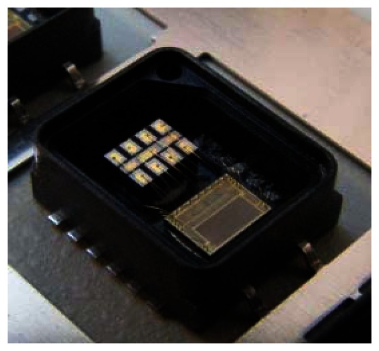
MEMS based Accelerometer (VTI Inc.).

Among the applications of MEMS technology, MEMS- based inertial sensors such as MEMS based gyroscopes and MEMS based accelerometers have been adopted as aiding sensors to improve navigation information continuity. While the MEMS based gyroscope is a relatively new technology and still an ongoing research activity for commercial uses, the MEMS based accelerometer has been widely utilized in a variety of developments and its success is significant.

In the navigation field, it has been reported that many efforts have been made to make the smaller and less expensive navigation devices available for more users. MEMS based inertial sensors have recently drawn great attention as aiding GPS outages with low inherent cost, small size, low power consumption, and solid reliability. However, their performance is still considered poor in accuracy for certain applications. In this paper, the MEMS based inertial sensors' performance will be investigated and a land vehicle navigation system prototype will be developed by integrating MEMS based inertial sensors, a low cost GPS receiver and a digital compass.

In spite of the smaller size and cost effectiveness of MEMS based inertial sensors, the error behaviour of MEMS based inertial sensors must be appropriately treated in order to turn the raw sensor measurements into reliable and useful data for vehicle position determination. When we confine the scope of application of MEMS based inertial sensors to aiding GPS solutions to a relatively short period of time, some deterministic error sources (zero-offset bias and 1^st order scale factor) and stochastic variation (random noise) can be considered as the main concerns to be discussed among the different types of error sources for MEMS based inertial sensors. Besides, the understanding of their stochastic variations is of significant importance for the development of optimal estimation algorithms.

In the subsequent sections, the conventional error model of inertial sensors will be simplified considering MEMS based sensor design and a short time period usage assumption. The deterministic error sources will be estimated by using multi-position test which is well described in the reference [2], and the stochastic variation will be modeled by 1^st order Gauss-Markov (GM), which has been widely used in navigation field, and a higher order AutoRegressive (AR) model introduced in [3]. The deterministic error sources (zero-offset bias and 1^st order scale factor) of MEMS based inertial sensors estimated by using multi-position testing in the laboratory will be referenced to initial measurement in kinematic environments. For the stochastic variation, not only the conventional 1^st order GM model but also a higher order AR model will be used in optimal estimation algorithm (i.e. Kalman filter) to quantify the effect of precise stochastic modeling method for MEMS based inertial sensor applications in kinematic environments. When the performance of MEMS-based inertial sensors are admissible for a certain application such as land vehicle navigation, a continuous integrated navigation system will be available by integrating GPS with cheaper and smaller inertial sensors in urban canyons with GPS signal blockages.

2. Accelerometer/Gyroscope Error Model and Stochastic Modeling

There are two major aspects that should be considered in the error analysis of any MEMS-based sensor: (1) error analysis to identify deterministic error and non-deterministic (stochastic) error sources; and (2) the development of stochastic modeling methods used to characterize the random part of the sensor output.

2.1. Error Sources and Error Models

Current commercial accelerometers/gyroscopes are mainly classified as either mechanical or solid-state. As mentioned before, all accelerometers/gyroscopes are suffering from a variety of error sources which are slightly different depending upon different types of the manufacturing principles. The error equation of conventional mechanical inertial sensors from the reference [2] will be first introduced and the error equation will then be simplified according to the tolerance of a specific application such as land vehicle navigation system and MEMS technology.

Conventionally, the measurement in the X-axis provided by accelerometer ( ã_x ) can be expressed in terms of the applied acceleration acting along its sensitive axis ( a_x ) and the accelerations acting along the pendulum and hinge axes, a_y and a_z respectively, by the equation [2]:

$${\tilde{a}}_x=(1+S_x)a_x+M_y{a}_y+M_z{a}_z+B_f+B_v{a}_x{a}_y+n_x$$ (1)

where S_x is the scale factor error, usually expressed in polynomial form to include non-linear effects, M_y ,M_z are the cross-axis coupling factors, B_f is the measurement zero-offset bias, B_v is the vibro-pendulous error coefficient, and n_x is the random noise.

For an accelerometer based on MEMS technology and non-pendulous design, it is reasonable to expect that the cross-axis coupling factors and vibro-pendulous error would be insignificant because most MEMS accelerometers are assembled as three single-axis accelerometers so that they have low cross-axis coupling factors [4]. Then, the conventional error model can be simplified as below,

$${\tilde{a}}_x=a_x+S_x{a}_x+B_f+n_x$$ (2)

As indicated by Equation (2), the zero-offset bias and the 1^st order scale factor are the main concerns for the deterministic error sources and the last term is the stochastic variation of the sensor output. The Y-axis and Z-axis measurements can be expressed in the same way.

Similarly, current commercial gyroscopes utilize different development principles, resulting in various types of gyroscopes with distinct characteristics for each one. Accordingly, assuming the acceleration sensitive errors are negligible, the measured angular rate can be modeled for many applications as [2]

$${\tilde{\omega }}_z=(1+S_z){\omega }_z+M_x{\omega }_x+M_y{\omega }_y+B_f+n_z$$ (3)

where S_x is the scale factor which may be expressed as a polynomial in ^ωz to represent scale factor non-linearity, M_y ,M_z are the cross-axis coupling factors, B_f is the measurement zero-offset bias, n_z is the random noise. Using the same assumption in the accelerometer case, Equation (3) can be simplified as

$${\tilde{\omega }}_z={\omega }_z+S_z{\omega }_z+B_f+n_z$$ (4)

in which only the zero-offset bias and 1^st order scale factor are included with significant contribution to the deterministic error sources. Equations (2) and (4) will be used to estimate the deterministic error sources (zero-offset bias and 1^st order scale factor) by using multi-position testing.

2.2. Stochastic Modeling

Considering only linear stationary stochastic processes, one way to specify a random process is to describe in detail the conceptual chance experiment giving rise to the process [5]. As it can be seen, many signals are quite different, even with same mean and variance values, so it is clear that more information than just mean and variance is needed in order to describe the random process more precisely. It has been seen that the autocorrelation function, denoted as R_X (τ) in the sequel, is an important descriptor of a random process that is relatively easy to obtain because it depends on only the second-order probability density for the process [5]. Thus, if R_X (τ) is known a-prior or if we can estimate R_X (τ) from observational data, then we can use this information to help “identify” which of the special models (if any) would fit the process under study [6].

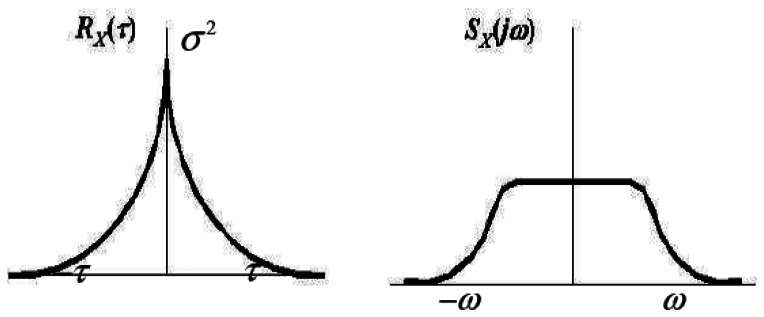
If a stationary Gaussian process X_t has an exponential Autocorrelation, it is called a Gauss-Markov (GM) process. As shown in Figure 2, the autocorrelation and spectral functions of 1^st order GM process have the form of

$$\begin{array}{cc}& R_X(\tau )={\sigma }^2{e}^{-\beta \left|\tau \right|}\\ S_X(j\omega )=\frac{2{\sigma }^2\beta }{{\omega }^2+{\beta }^2}& \left[\text{or}{S}_X(s)=\frac{2{\sigma }^2\beta }{-s^2+{\beta }^2}\right]\end{array}$$ (5)

Figure 2.

Autocorrelation and FFT Transform of 1^st Order Gauss Markov Process

The mean-square value and time constant for the process are given by the σ² and 1/β parameters, respectively. The Gauss-Markov process is a very useful process in applied work because (i) it can fit a large number of physical processes with reasonable accuracy, and (ii) it has a relatively simple mathematical description. In positioning and navigation fields, 1^st order Gauss-Markov process has been frequently used to describe the stochastic behaviors due to its simple estimation.

However, quite often even with simple representation of time-correlated signal behaviour, the estimated autocorrelation and its FFT transform are quite different from 1^st order Gauss-Markov process shown in Figure 2. Considering the very noisy measurements and poor performance of MEMS based inertial sensors, the more precise and appropriate stochastic modeling is desirable. In this paper, a higher order AutoRegressive model will be applied and compared with 1^st order Gauss-Markov process.

Some of special discrete parameter stochastic models which can provide us with a structure for fitting models to practical data have been studied in probability and mathematical statistics theory such as the purely random noise {ε_t}, the AutoRegressive model (AR), the MovingAverage model (MA), the mixed AutoRegressive/MovingAverage model (ARMA), the harmonic model, just to mention a few. Among the discrete parameter stochastic models, AR model has been widely adopted to describe random noise output of physical systems in many fields because the relatively simple parameter estimation and the value of {ε_t } is “drawn into” the process {X_t } and thus influences all future values, X_t, X_t+1, X_t+2, ...... resulting in its autocorrelation function “dies out gradually” [6]. The attempt to apply AR model for inertial sensors was first introduced in [3] and its mathematical description can be found in [3][6][7][8].

With the standard form of AR model,

$$X_t+a_1{X}_{t-1}+\dots +a_k{X}_{t-k}={\varepsilon }_t$$ (6)

$$H(z)=\frac{E(z)}{X(z)}=\frac{b_0}{1+\text{∑}_{k=1}^N{a}_k{z}^{-k}}$$ (7)

where b₀ is the variance ${\sigma }_{\varepsilon }^2$ of ε_t which represents a random process. For a variety of methods to estimate the parameters a_k the reader is referred to the literature ([6], [7]) and this paper will apply one of them. Also, if the process is both causal and stable, then all the poles of H(z) must lie inside the unit circle of the z-plane because the Region of Convergence (ROC) is of the form | z | > r_max, and since the unit circle is included in the ROC, one must have r_max < 1, where r_max equals the largest magnitude of any of the poles of H(z) [9].

The most considered AR model based parameter estimation methods are the Yule-Walker, Burg and Unconstrained Least-Squares methods [7]. For a large dataset, the results of these three different methods provide a fairly close estimation results of the parameters. However, there are still some different characteristics for each method to be noticed. The authors chose the Burg method, which is quite popularly used and estimates the reflection coefficients by minimizing both forward and backward prediction errors in the least square sense with the constraint that the AR parameters satisfy the Levinson-Durbin recursion. Unless a priori information about the order of an AR Model was given, the order of the AR model is an unknown, so it needs to be estimated. Several method to determine the order of the AR Model have been reported in literatures such as Final Prediction Error (FPE), Akaike's Information Criterion (AIC), Minimum Description Length (MDL), Investigation of Residual Variance (IRV) and etc. One of the common ways to determine the order of the AR model is to investigate the residual variance for different orders. Assuming the true model is of finite order, as the estimated order is getting close to the true model, the residual variance wouldn't reduce significantly [7]. It should be kept in mind that a higher order AR model would increase Kalman Filter error states. As a result, it would increase the computational loads and might result in unstable solutions [3].

3. Performance Analysis Methodology

3.1. Kinematic Testing System Configuration

The kinematic testing has been conducted to qualify the performance of the integrated system of MEMS based inertial sensor (RGA300CA) and the low-cost GPS receiver module (Leadtek GPS-9543) utilizing different stochastic modeling schemes (4^th order AR model and 1^st order Gauss-Markov model). It is a simplified navigation testing with the assumptions that the testing area is 2-dimensional, flat (nominal roll/pitch) and non-accelerating (short testing duration). Also, the initial misalignment is assumed to be negligible. For the initial position and heading information, a dual frequency GPS receiver (Javad Legacy GPS receiver) and a digital compass (Honeywell HMR-3300) have been used and the measurements from the high precision Javad Legacy GPS receiver were also processed to generate the reference trajectory shown in Figures 3 and 4.

Figure 3.

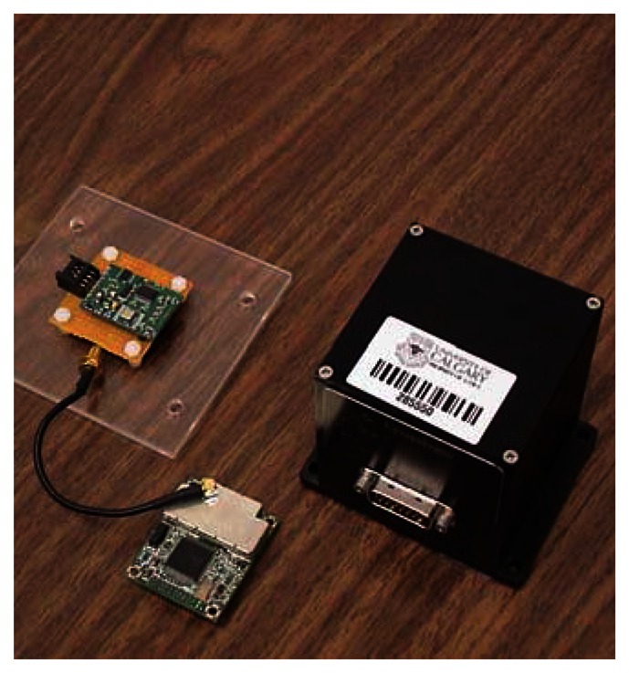
Kinematic Testing Sensors.

Figure 4.

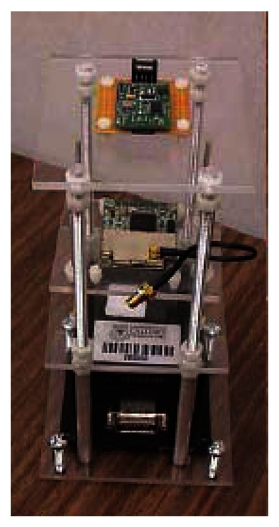
Testing Installation.

Two GPS antennas (Javad Legacy and Leadtek GPS 9531) were mounted on the roof of the testing van and the testing system was held tight inside the vehicle. Two laptop computers were needed to record the reference GPS measurements and integrated system with different acquisition S/W separately. Table 1 summarizes the basic specifications of each sensor in the testing system.

Table 1.

System Specifications (Courtesy of Crossbow, Leadtek, Honeywell Inc.).

RGA300CA
Angular Rate		Acceleration
Range: Yaw (°/sec)	±100	Range: X/Y/Z (g)	±2
Bias: Yaw (°/sec)	<±2.0	Bias: X/Y/Z (mg)	<±30
Scale Factor Accuracy (%)	<1	Scale Factor Accuracy (%)	<1
Non-Linearity (%FS)	<0.3	Non-Linearity (%FS)	<1
Resolution (°/sec)	<0.025	Resolution (mg)	<1.0
Bandwidth (Hz)	>25	Bandwidth (Hz)	>50
Random Walk (°/hr1/2)	<2.25	Random Walk (m/s/hr1/2)	<0.15
GPS-9543		HMR3300
Main Chip	SiRF star II	Heading Accuracy	1°
Tracking Channel	12	Resolution	0.1°
L1 Frequency (MHz)	1575.42 C/A code	Repeatability	0.5°
Position Accuracy (m)	10, 2D
Input Massage	NMEA/SiRF Binary
Output Massage	SiRF Binary + NMEA-0183
Time Mark	Output 1pps

3.2. Testing Dataset and Data Processing

The testing dataset is composed of three different system files and one reference GPS file. The system files are using the same computer time. For the field testing, the system will include about 20 minutes warming-up period, the compass calibration period, the static motion period, and the kinematic motion period. After the warming period, a digital compass will be calibrated using 360° rotation circle motion each time and then, at least 5 minutes static collection will be made. It would have been done this way because on/off zero-offset bias should be examined before actual kinematic data processing. The total kinematic testing duration was limited to 10 minutes and the same testing routine was conducted 10 times.

For the initial heading, the digital compass output will be used considering the discrepancy between magnetic north and geodetic north. The term “magnetic north” refers to the position of the earth's magnetic pole and it differs from a geodetic north. The angle between magnetic north and the geodetic north direction is called magnetic declination. As the magnetic declination does not remain constant in time, it needs to be referred to a recent geographic lookup table or geodetic services available in order to add or subtract the proper declination angle to correct for the geodetic north with certain accuracy. Natural Resources of Canada (NRCan) provides a recent estimation of the declination based on Canadian Geomagnetic Reference Field (CGRF) which is a model of the magnetic field over the Canadian region. As a result, a declination angle of 17.183° E was obtained through the University of Calgary campus with 0.5° accuracy and added to the initial heading from HMR3300 magnetic compass.

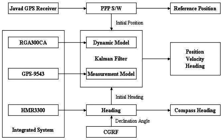
The initial position will be provided through the processing of the Javad Lagacy GPS receiver measurements using the Precise Point Positioning (PPP) software package P^3TM developed at The University of Calgary. The PPP position solutions have centimeter to decimeter accuracy, providing a reference trajectory to assess the performance of the integrated system. The data processing associated with kinematic testing is illustrated in Figure 5. The trajectory generated by the integrated system will be compared with the reference trajectory using GPS time synchronization. The same data processing will be conducted for two different stochastic modeling schemes (GM vs. AR).

Figure 5.

Data Processing Flow.

3.3. Mathematical Error Model

The Kalman filter mathematical derivation for 2-dimensional testing using X/Y accelerometer and yaw rate measurements along with GPS position updates is followed below based on the discussion in the reference [10].

$$\left[\begin{array}{c}\dot{n}\\ \dot{e}\\ {\dot{v}}_n\\ {\dot{v}}_e\\ \dot{\psi }\end{array}\right]=\left[\begin{array}{c}{v}_n\\ v_e\\ cos(\psi ){\alpha }_u-sin(\psi ){\alpha }_v\\ sin(\psi ){\alpha }_u-cos(\psi ){\alpha }_v\\ {\omega }_r\end{array}\right]=\left[\begin{array}{c}{v}_n\\ v_e\\ {\alpha }_n\\ {\alpha }_e\\ {\omega }_r\end{array}\right]$$ (8)

where [n,e] are the position coordinates in north and east directions and [v_n,v_e ] are the corresponding velocities; [a_n,a_e] and [a_u,a_v] are the measured accelerations in the navigation and body frames, respectively; ψ is yaw angle and ω_r is the measured yaw rate in the body frame, and

$$\left[\begin{array}{c}{\alpha }_n\\ {\alpha }_e\end{array}\right]=\left[\begin{array}{cc}cos(\psi )& -sin(\psi )\\ sin(\psi )& cos(\psi )\end{array}\right]\left[\begin{array}{c}{\alpha }_u\\ {\alpha }_v\end{array}\right]$$ (9)

When the bias errors are modeled in each of the sensors,

$$\begin{array}{c}{\tilde{\alpha }}_u={\alpha }_u+\delta {\alpha }_u\\ {\tilde{\alpha }}_v={\alpha }_v+\delta {\alpha }_v\\ {\tilde{\omega }}_r={\omega }_r+\delta {\omega }_r\end{array}$$ (10)

and the actual mechanization system is modeled as

$$\left[\begin{array}{c}\dot{\widehat{n}}\\ \dot{\widehat{e}}\\ {\dot{\widehat{v}}}_n\\ {\dot{\widehat{v}}}_e\\ \dot{\widehat{\psi }}\end{array}\right]=\left[\begin{array}{c}{\widehat{v}}_n\\ {\widehat{v}}_e\\ cos(\widehat{\psi }){\tilde{\alpha }}_u-sin(\widehat{\psi }){\tilde{\alpha }}_v\\ sin(\widehat{\psi }){\tilde{\alpha }}_u+cos(\widehat{\psi }){\tilde{\alpha }}_v\\ {\tilde{\omega }}_r\end{array}\right]$$ (11)

Linearization about the trajectory results in the following set of equations,

$$\begin{array}{c}\left[\begin{array}{c}\delta \dot{n}\\ \delta \dot{e}\\ \delta {\dot{v}}_n\\ \delta {\dot{v}}_e\\ \delta \dot{\psi }\end{array}\right]\end{array}=\left[\begin{array}{ccccc}0& 0& 1& 0& 0\\ 0& 0& 0& 1& 0\\ 0& 0& 0& 0& -{\alpha }_e\\ 0& 0& 0& 0& {\alpha }_n\\ 0& 0& 0& 0& 0\end{array}\right]\left[\begin{array}{c}\delta n\\ \delta e\\ \delta v_n\\ \delta v_e\\ \delta \psi \end{array}\right]+\left[\begin{array}{ccc}0& 0& 0\\ 0& 0& 0\\ cos(\psi )& -sin(\psi )& 0\\ sin(\psi )& cos(\psi )& 0\\ 0& 0& 1\end{array}\right]\left[\begin{array}{c}\delta {\alpha }_u\\ \delta {\alpha }_v\\ \delta {\omega }_r\end{array}\right]$$ (12)

Expanding Equation (12) to include the bias errors as the error states which are modeled as random constant process, we have the following dynamic equation:

$$\left[\begin{array}{c}\delta \dot{n}\\ \delta \dot{e}\\ \delta {\dot{v}}_n\\ \delta {\dot{v}}_e\\ \delta \dot{\psi }\\ \delta {\dot{\alpha }}_u\\ \delta {\dot{\alpha }}_v\\ \delta {\dot{\omega }}_r\end{array}\right]=\left[\begin{array}{cccccccc}0& 0& 1& 0& 0& 0& 0& 0\\ 0& 0& 0& 1& 0& 0& 0& 0\\ 0& 0& 0& 0& -{\alpha }_e& cos(\psi )& -sin(\psi )& 0\\ 0& 0& 0& 0& {\alpha }_n& sin(\psi )& cos(\psi )& 0\\ 0& 0& 0& 0& 0& 0& 0& 1\\ 0& 0& 0& 0& 0& 0& 0& 0\\ 0& 0& 0& 0& 0& 0& 0& 0\\ 0& 0& 0& 0& 0& 0& 0& 0\end{array}\right]=\left[\begin{array}{c}\delta n\\ \delta e\\ \delta v_n\\ \delta v_e\\ \delta \psi \\ \delta {\alpha }_u\\ \delta {\alpha }_v\\ \delta {\omega }_r\end{array}\right]$$ (13)

Denote the coefficient matrix in Equation (13) as F, the corresponding transition matrix can be approximated by the following equation:

$${\Phi }_{\mathit{\text{INS}}}=I+F\Delta t$$ (14)

The discrete form of Equation (13) becomes

$$\left[\begin{array}{c}\delta n_k\\ \delta e_k\\ \delta v_{nk}\\ \delta v_{ek}\\ \delta {\psi }_k\\ \delta {\alpha }_{uk}\\ \delta {\alpha }_{vk}\\ \delta {\omega }_{rk}\end{array}\right]=\left[\begin{array}{cccccccc}1& 0& \Delta t& 0& 0& 0& 0& 0\\ 0& 1& 0& \Delta t& 0& 0& 0& 0\\ 0& 0& 1& 0& -{\alpha }_e\Delta t& cos(\psi )\Delta t& -sin(\psi )\Delta t& 0\\ 0& 0& 0& 1& {\alpha }_n\Delta t& sin(\psi )\Delta t& cos(\psi )\Delta t& 0\\ 0& 0& 0& 0& 1& 0& 0& \Delta t\\ 0& 0& 0& 0& 0& 1& 0& 0\\ 0& 0& 0& 0& 0& 0& 1& 0\\ 0& 0& 0& 0& 0& 0& 0& 1\end{array}\right]\left[\begin{array}{c}\delta n_k-1\\ \delta e_k-1\\ \delta v_{nk}-1\\ \delta v_{ek}-1\\ \delta {\psi }_k-1\\ \delta {\alpha }_{uk}-1\\ \delta {\alpha }_{vk}-1\\ \delta {\omega }_{rk}-1\end{array}\right]$$ (15)

Now, the accelerometer bias errors and gyroscope bias error will be modeled by GM and AR methods separately with the estimated values based on multi-position testing. Note that the random white noise vectors associated with the dynamic equations have not shown in the above derivations.

4. Multi-Position Testing

RGA300CA system consists of a MEMS angular rate gyro and a triaxial silicon MEMS accelerometer. The triaxial accelerometer is a bulk-micromachined capacitive accelerometer whose input range is ±2g.

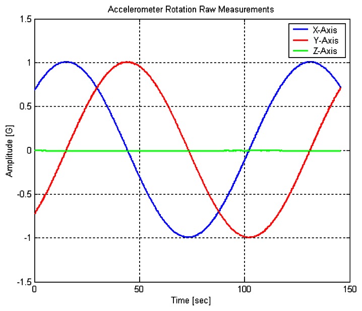
First, RGA300CA has been tested in the rotation panel connected to SmartMotor from Animatics Corporation. The testing rate table was carefully leveled relative to the local gravity vector. Once an accelerometer was attached to the testing rate table properly, the accelerometer output was collected with constant speed of rotation. The actual measurements of X/Y/Z axes of the accelerometer were compared with the reference acceleration determined by the testing rate table orientation. Using the error model described in the previous section and the “best fit” line regression method, the deterministic error sources have been estimated and used for calibration. Both of accelerometer and rotation panel were turned on and off every time with about 10 minutes apart and were warmed up for about 5 minutes before each datalogging [11]. The room temperature (about 21°C) was also monitored. The local gravity value (9.8080.m/s²) in the Multi-Sensor Lab at the University of Calgary has been used for the reference gravity value. One set of the accelerometer measurements coinciding z-axis with rotation axis of rate table is shown in Figure 6.

Figure 6.

RGA300CA Accelerometer Measurements.

For the sensor, 20 Hz logging rate and approximate bandwidth 10 Hz were used with data logging systems as GYRO-VIEW from Crossbow for RGA300CA. Also, the model SM2330SQ version 4.11 motor was used with SMI 1.310 windows S/W from Animatics. The RGA300CA and the rotation panel were connected to separate computers with RS-232 port cables and the output of the sensor measurements was saved in text file format.

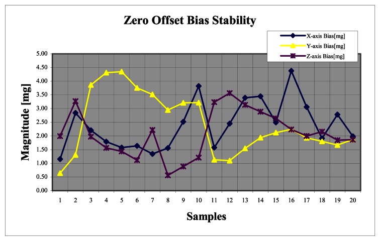
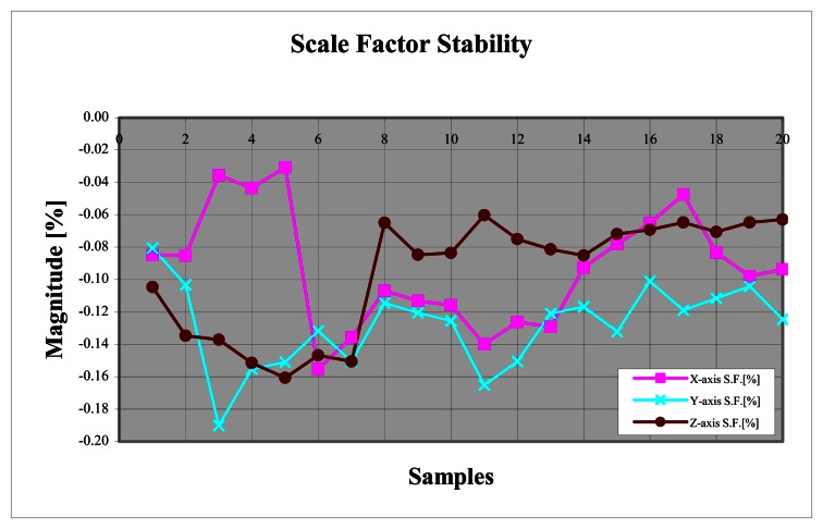
Due to the instability of the rotating motor and the initial alignments, the angular velocity should be calculated for every run. The zero-offset bias ( B_f ) and 1^st order scale factor ( S_x ) can be obtained by using Least Squares method with rotational measurements and reference gravity value. The bias and the scale factor stability results are given in Figures 7 and 8 with their mean & standard deviation shown in Table 2.

Figure 7.

Accelerometer Zero Offset Bias Stability.

Figure 8.

Accelerometer 1^st order Scale Factor Stability.

Table 2.

Bias and Scale Factor Results.

	X-axis		Y-axis		Z-axis
	Bias[mg]	S.F.[%]	Bias[mg]	S.F.[%]	Bias[mg]	S.F.[%]
Mean	2.3961	-0.093	2.4233	-0.1284	2.0901	-0.0962
St.D.	0.8858	0.0358	1.1304	0.0256	0.8356	0.0357

As discussed in the previous section, the deterministic error sources of RGA300CA Yaw rate gyroscope are zero-offset bias and 1^st order scale factor. Analogous to the accelerometer case, the simplified form of error Equation (4) without any modification will be used to analyze the actual gyroscope's Yaw rate measurements. This time, the rotational table has been precisely leveled out horizontally to provide the reference angular rate which is supposed to be correspondent to Yaw rate of gyroscope assuming that Earth rotation rate effect is nominal.

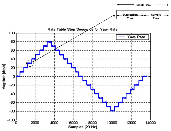
During a typical test schedule, the rotation rate of the rate table is stepped through a series of angular rates starting from zero deg/s recording data at each stage. The rotation speed is kept constant for a period at each step and the sensor outputs are allowed to stabilize, before recording the output signals. The applied angular rate is varied in incremental steps between the maximum and minimum desired rotation rates. At each step, the signals from gyroscope are recorded when the sensor is in equilibrium [2].

In this experiment, the applied rotation rate has been increased from 0 deg/s to 80 deg/s and then, decreased until negative 80 deg/s. After that, it resumed to increase from -80 deg/s to 0 deg/s. For each rotation rate steps (10 deg/s), the dwell time consists of stabilization time (about 10 seconds) and sample time (about 10 seconds). 33 subsets of data have been recorded based on the same scheme and combined together to compose a series of measurements. One of the testing results has been illustrated in Figure 9.

Figure 9.

RGA300CA Gyroscope Measurements.

Those recorded data has been averaged out to provide a list of measurements resulting in measurement matrix in Least Squares estimation scheme. Accordingly, two parameters (zero-offset bias and 1^st order scale factor) could be estimated by simple Least Squares process with 33 measurements. The same test has been performed ten times with approximately 30 minutes interval. The results of the ten tests with their mean & standard deviation for Yaw-rate are shown in Table 3. The mean values of Table 2 and Table 3 will be referred in the initial static leveling in kinematic testing.

Table 3.

Bias and Scale Factor Results of Gyroscope (Yaw-Rate).

	Bias[d/s]	S.F.[%]
1	0.2359	-0.3837
2	0.2284	-0.3977
3	0.2469	-0.3693
4	0.2206	-0.4164
5	0.2990	-0.4538
6	0.3164	-0.3154
7	0.3071	-0.4203
8	0.3180	-0.4367
9	0.3310	-0.3462
10	0.3095	-0.4445
Mean	0.2813	-0.3984
St.D.	0.0407	0.0449

5. Stochastic Modeling of RGA300CA

Based on the discussion in previous sections, the stochastic variation (random noise) of the experimental output of accelerometer and gyroscope inside RGA300CA will be analyzed and modeled appropriately. Since the usage of 1^st Gauss-Markov model is well known in many literatures, only the stochastic modeling by AutoRegressive model will be described here. AR model parameters will be estimated by using Burg method and corresponding order of AR model will be approximated by investigating the residual variance in accordance to different orders considering the increase of state vector in Kalman Filter error state.

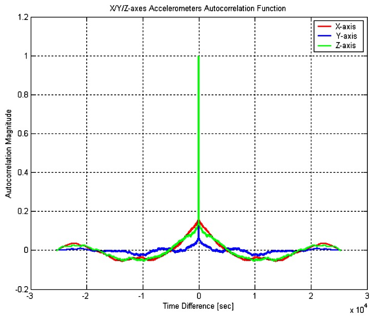
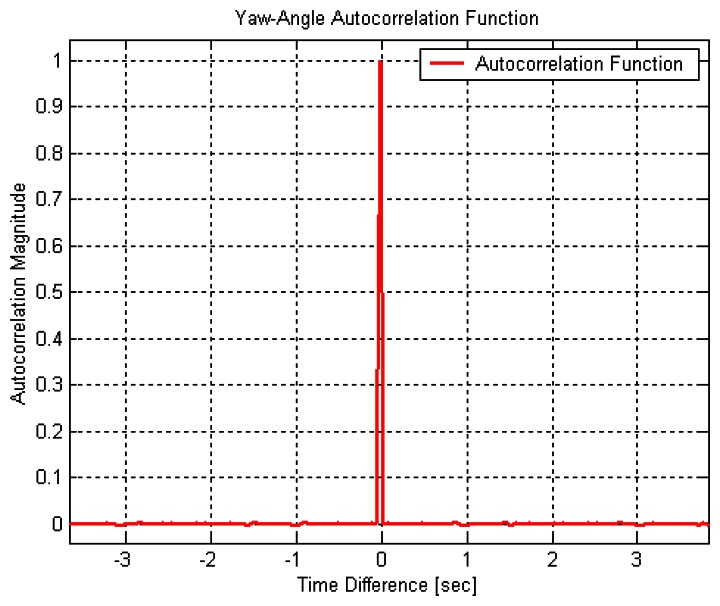
Shown in Figures 10 and 11 are the normalized autocorrelation functions of a triaxial accelerometer and yaw rate gyroscope outputs in well-leveled static mode with about 3 hours warming time. It is clear that the temperature variation of the sensor unit affects the sensor measurements significantly. It is well indicated in many literatures that the temperature is the main concern of sensor output stability. That is why measurements after three hours were being used for the analysis. Therefore, the relatively stable parts of the original accelerometer/gyroscope measurements were only used and their trends were removed.

Figure 10.

Estimated Autocorrelation Functions of tri-axial Accelerometer Measurements.

Figure 11.

Estimated Autocorrelation Function of Gyroscope Measurements.

As expected, the RGA300CA measurements have shown very short correlation times in Figures 10 and 11. For the gyroscope, its stochastic variation has behaved as quite purely random process (white noise). On the other hand, Figure 10 has indicated that there exists time correlated behaviour in the stochastic variation of the accelerometer measurements and it should be modeled precisely.

There are two main steps involved in AR modeling, namely, parameter estimation and order determination. Once the three parameter estimation methods in the previous section were performed to estimate the parameters using the sample dataset (about 8 hours with a sampling rate of 20Hz), they have provided very close results from one to the other. Therefore, in spite of some distinct characteristics, any methods could be used in this experiment.

In the testing, the Burg method has been applied. To assess the proper determination of the order for AR model, the estimated residual variance ${\sigma }_{\varepsilon }^2$ in accordance to different orders was chosen to be analyzed. In order to avoid abrupt increase in the error states of the Kalman filter due to the increase of the order of the AR model, an appropriate order ought to be determined when the variance plot starts to be leveled out in Figure 12.

Figure 12.

Estimated Residual Variance Plot with Different Orders of AR model for Accelerometer.

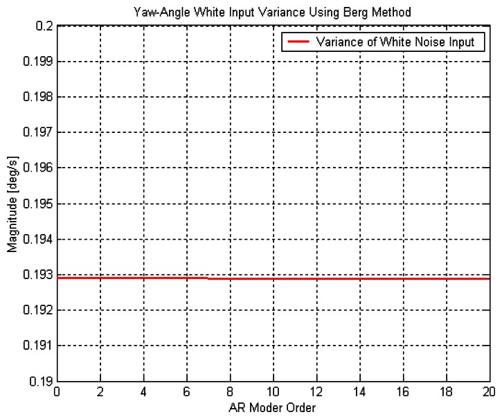
Based on the results shown in Figures 12 and 13, a 4^th order AR model for the stochastic variation of the accelerometer has been chosen and its parameters were estimated by the Burg method. A total of 10 sample datasets have been used for the estimation of the AR model parameters and the mean values will be used for bias modeling in optimal estimation algorithm for kinematic testing. Therefore, the stochastic variation of accelerometer output will be modeled by 1^st order GM and 4^th AR models and the stochastic variation of gyroscope output will be modeled by purely random process (white noise) based on Figure 11 and 13. Now the error state vector includes 14 states, namely 2 for position, 2 for velocity, 1 for misalignment, 8 for 4^th order AR model of X/Y-axis of accelerometer biases and 1 for white noise for yaw rate bias. The corresponding dynamic model driven by the white noise w and the measurement model equations have the expressions as follows:

$$\left[\begin{array}{c}\delta n_k\\ \delta e_k\\ \delta v_{nk}\\ \delta v_{ek}\\ \delta {\psi }_k\\ \delta {\alpha }_{uk}\\ \delta {\alpha }_{uk-1}\\ \delta {\alpha }_{uk-2}\\ \delta {\alpha }_{uk-3}\\ \delta {\alpha }_{vk}\\ \delta {\alpha }_{vk-1}\\ \delta {\alpha }_{vk-2}\\ \delta {\alpha }_{vk-3}\\ \delta {\omega }_{rk}\end{array}\right]=\left[\begin{array}{cccccccccccccc}1& 0& \Delta t& 0& 0& 0& 0& 0& 0& 0& 0& 0& 0& 0\\ 0& 1& 0& \Delta t& 0& 0& 0& 0& 0& 0& 0& 0& 0& 0\\ 0& 0& 1& 0& -{\alpha }_e\Delta t& cos(\psi )\Delta t& 0& 0& 0& -sin(\psi )\Delta t& 0& 0& 0& 0\\ 0& 0& 0& 1& {\alpha }_n\Delta t& sin(\psi )\Delta t& 0& 0& 0& cos(\psi )\Delta t& 0& 0& 0& 0\\ 0& 0& 0& 0& 1& 0& 0& 0& 0& 0& 0& 0& 0& \Delta t\\ 0& 0& 0& 0& 0& -a_{u1}& -a_{u2}& -a_{u3}& -a_{u4}& 0& 0& 0& 0& 0\\ 0& 0& 0& 0& 0& 1& 0& 0& 0& 0& 0& 0& 0& 0\\ 0& 0& 0& 0& 0& 0& 1& 0& 0& 0& 0& 0& 0& 0\\ 0& 0& 0& 0& 0& 0& 0& 1& 0& 0& 0& 0& 0& 0\\ 0& 0& 0& 0& 0& 0& 0& 0& 0& -a_{v1}& -a_{v2}& -a_{v3}& -a_{v4}& 0\\ 0& 0& 0& 0& 0& 0& 0& 0& 0& 1& 0& 0& 0& 0\\ 0& 0& 0& 0& 0& 0& 0& 0& 0& 0& 1& 0& 0& 0\\ 0& 0& 0& 0& 0& 0& 0& 0& 0& 0& 0& 1& 0& 0\\ 0& 0& 0& 0& 0& 0& 0& 0& 0& 0& 0& 0& 0& 0\end{array}\right]\left[\begin{array}{c}\delta n_{k-1}\\ \delta e_{k-1}\\ \delta v_{nk-1}\\ \delta v_{ek-1}\\ \delta {\psi }_{k-1}\\ \delta {\alpha }_{uk-1}\\ \delta {\alpha }_{uk-2}\\ \delta {\alpha }_{uk-3}\\ \delta {\alpha }_{uk-4}\\ \delta {\alpha }_{vk-1}\\ \delta {\alpha }_{vk-2}\\ \delta {\alpha }_{vk-3}\\ \delta {\alpha }_{vk-4}\\ \delta {\omega }_{rk-1}\end{array}\right]+\left[\begin{array}{c}0\\ 0\\ 0\\ 0\\ 0\\ w_{uk}\\ 0\\ 0\\ 0\\ w_{vk}\\ 0\\ 0\\ 0\\ w_{\omega k}\end{array}\right]$$ (16)

$$\left[\begin{array}{c}{z}_n\\ z_e\end{array}\right]=\left[\begin{array}{cccccccccccccc}1& 0& 0& 0& 0& 0& 0& 0& 0& 0& 0& 0& 0& 0\\ 0& 1& 0& 0& 0& 0& 0& 0& 0& 0& 0& 0& 0& 0\end{array}\right]\left[\begin{array}{c}\delta n_k\\ \delta e_k\\ \delta v_{nk}\\ \delta v_{ek}\\ \delta {\psi }_k\\ \delta {\alpha }_{uk}\\ \delta {\alpha }_{uk-1}\\ \delta {\alpha }_{uk-2}\\ \delta {\alpha }_{uk-3}\\ \delta {\alpha }_{vk}\\ \delta {\alpha }_{vk-1}\\ \delta {\alpha }_{vk-2}\\ \delta {\alpha }_{vk-3}\\ \delta {\omega }_{rk}\end{array}\right]+v_k$$ (17)

Figure 13.

Estimated Residual Variance Plot with Different Orders of AR model for Gyro.

Again, the parameter estimation results in the multi-position testing have been used to construct the state transition matrix and the covariance matrix (Q ) associated with w_k in the dynamic model while the covariance matrix (R) associated with v_k in the measurement model has been constructed by using RMS values of GPS trajectory accuracy compared with PPP solutions.

6. Kinematic Testing and Results

To fulfill the testing assumptions described previously the kinematic testing has been conducted in one of the parking lots in the University of Calgary which is a relatively flat and open area. The vehicle was driven at speeds of 10 to 30 km/hr with six major turns. Around the corners, the speed was reduced and then, was accelerated along the straight path comparatively. The same driving testing was repeated 10 times with the same routine of data collection in the same area.

As illustrated and also described previously, the data collection consists of two parts, namely, static mode and kinematic mode after warming up and compass calibration periods. The static mode dataset for about five minutes was referenced with zero-offset bias estimation which was explained in multi-position testing. With an initial position from PPP processing of GPS measurements and initial heading corrected by CGRF, a Kalman filter error estimation has been conducted which is composed of a dynamic model using measurements of X/Y axes of accelerometer, Yaw rate gyroscope of RGA300CA and a measurement model using measurements of GPS-9543 module. The trajectories of the integrated system using 4^th order AR model and 1^st order GM model were first generated with the 1-sec update interval and were then compared with the PPP solution trajectory and GPS-9543 solution trajectory. After that, the system trajectories were generated with 5-sec, 10-sec, 20-sec, 30-sec, 60-sec update intervals.

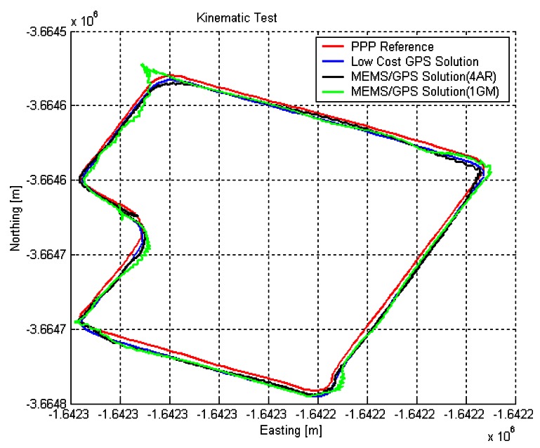
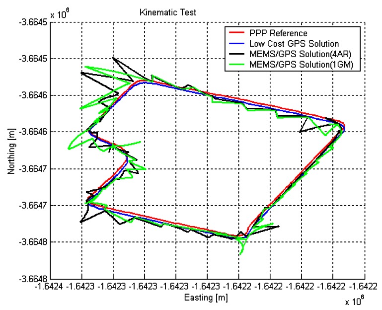
In the 1-sec update case, the system trajectories by both 4^th AR model and 1^st order GM model processes have indicated slightly better performance than the GPS-9543 solution. In the 5-sec, 10-sec, 20-sec update cases, the system solutions are showing that the position errors have increased significantly between updates. The biggest position errors have often occurred in the corner sections. This can be because the Yaw rate error is significant in position determination at the corners. Figures 14 and 15 illustrate the horizontal position trajectory for 1-sec update and 5-sec update intervals, respectively.

Figure 14.

Kinematic Testing Trajectory Plots (1-sec Updates).

Figure 15.

Kinematic Testing Trajectory Plots (5-sec Updates).

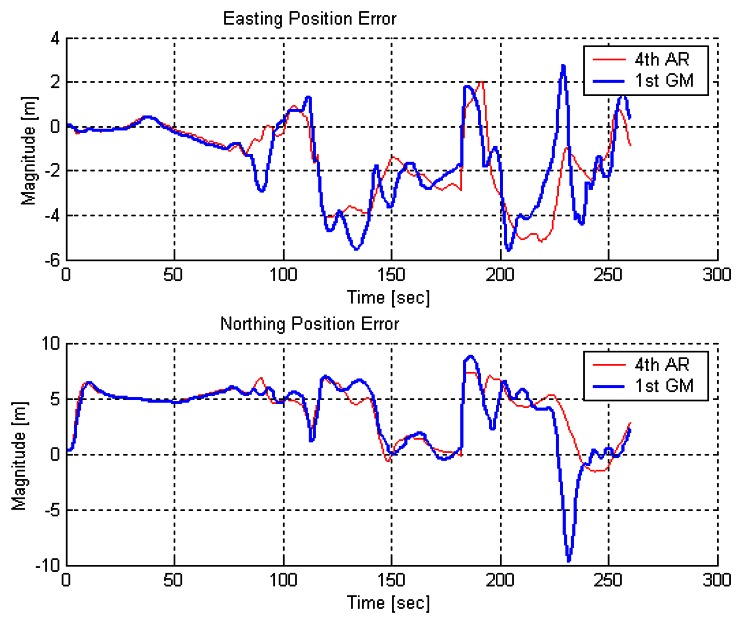
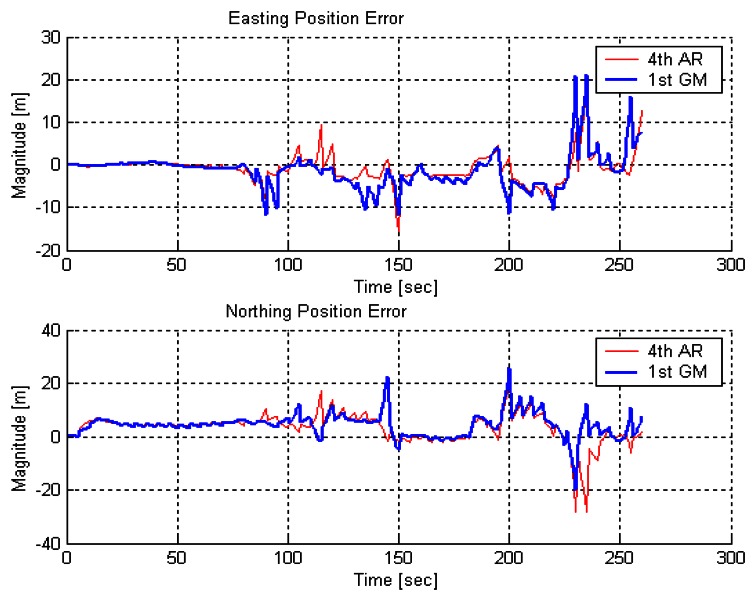
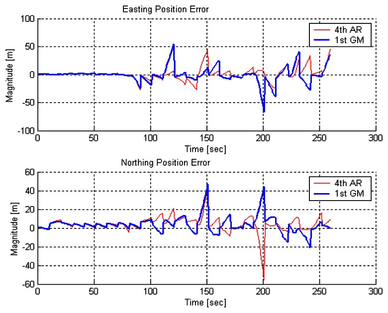
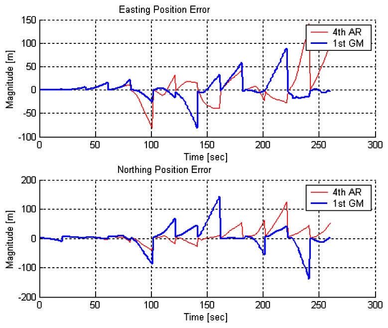
Shown in Figures 16, 17, 18 and 19 are northing and easting position errors from different updating intervals comparing to PPP solutions. It is noticed that the solutions of 4^th order AR model and 1^st order GM model are varying as the updating intervals have increased.

Figure 16.

Kinematic Testing Position Error Plots (1-sec Updates).

Figure 17.

Kinematic Testing Position Error Plots (5-sec Updates).

Figure 18.

Kinematic Testing Position Error Plots (10-sec Updates).

Figure 19.

Kinematic Testing Position Error Plots (20-sec Updates).

It is clear that the position error in each channel tends to increase without GPS position updates and settle down with updates. Also, the kinematic mode position error is much bigger than the static mode position error in all update interval cases. In the 10-sec updates, the maximum position error has reached to about 60 meters and even worse since 100 meter position error has been shown in the 20 sec updates. The numerical result of position errors of the kinematic testing is summarized in Table 4.

Table 4.

Kinematic Position Errors (m).

		X RMS	Y RMS	Hrioz.RMS
1-sec Update	4th AR Model	2.2643	4.5664	5.0970
	1st GM Model	2.3521	4.7023	5.2578
5-sec Update	4th AR Model	3.4984	6.5326	7.4104
	1st GM Model	4.5062	6.3012	7.7466
10-sec Update	4th AR Model	10.9184	9.5629	14.5142
	1st GM Model	13.6273	9.3777	16.5422
20-sec Update	4th AR Model	31.0981	25.9061	40.4749
	1st GM Model	22.6127	36.6627	43.0754
30-sec Update	4th AR Model	21.2120	76.1587	79.0575
	1st GM Model	60.9515	53.1926	80.8983
60-sec Update	4th AR Model	111.8538	165.9589	200.1340
	1st GM Model	276.4774	149.9599	314.5278

Based on the position error plots and numerical values in Table 4, the estimation with 4^th order AR model has produced better results than the estimation with 1^st order GM model in kinematic testing. However, the improvement is relatively smaller than the one in static testing [8]. It could be explained that the time-correlated behavior in the stochastic variation of MEMS inertial sensors are quite subtle and more unmodeled deterministic error sources are involved in the kinematic environments. This however is dependent on the testing equipments actually used in the testing.

The kinematic testing described here has made very important assumptions mentioned earlier. Therefore, the results with those assumptions and data processing method presented above should be understood very carefully.

6. Conclusions

The main purpose of this paper was to characterize the error behaviour of MEMS based inertial sensors and to analyze the performance of an integrated system prototype of MEMS based inertial sensors and a low-cost GPS receiver with digital compass. Along with deterministic error sources (zero-offset bias and 1^st order scale factor), the stochastic variation modeling of MEMS based inertial sensors was focused in this paper due to the assumption of short period of aiding time to GPS. The 1st order Gauss Markov and the 4^th order AR models have been used to model the stochastic variation of the MEMS accelerometers of RGA300CA. The static and kinematic tests have shown a better performance using the 4^th order AR model. However the test results have also demonstrated that the quality performance of MEMS based inertial sensors (RGA300CA) is not yet quite acceptable to aid GPS system for land vehicle application for longer period of GPS signal outrage. As the performance of MEMS sensors continues to improve, it is recommended to test the latest MEMS sensors available in the market to develop GPS/MEMS based inertial sensor integrated navigation system for continuous navigation solutions with the procedures described here.

References and Notes

- 1.Huff M.A. Position Paper: MEMS Manufacturing. The MEMS Exchange; Reston, Virginia, U.S.A.: 1999. [Google Scholar]
- 2.Titterton D.H., Weston J.L. Strapdown Inertial Navigation Technology. Peter Peregrinus Ltd.; UK: 1997. [Google Scholar]
- 3.Nassar S., Schwarz K.P., Noureldin A., El-Sheimy N. Modeling Inertial Sensor Errors Using Autoregressive (AR) Models. Proceedings of ION National Technical Meeting; Anaheim, CA, U.S.A.. 2003. [Google Scholar]
- 4.Allen J.J., Kinney R.D., Sarsfield J., Daily M.R., Ellis J.R., Smith J.H., Montague S., Howe R.T., Boser B.E., Horowitz R., Pisano A.P., Lemkin M.A., Clark W.A., Juneau C.T. Integrated Micro-Electro Mechanical Sensor Development for Inertial Application. Sandia National Laboratories; Albuquerque, NM, U.S.A.: 1998. [Google Scholar]
- 5.Brown R.G., Hwang P.Y.C. Introduction to Random Signals and Applied Kalman Filtering. Wiley; New York: 1997. [Google Scholar]
- 6.Priestley M.B. Spectral Analysis and Time Series. Academic Press; London: 2001. [Google Scholar]
- 7.Proakis J.G., Rader C.M., Ling F., Nikias C.L. Advanced Digital Signal Processing. Macmillan Publishing Company; New York, U.S.A.: 1992. [Google Scholar]
- 8.Park M. Error Analysis and Stochastic Modeling of MEMS based Inertial Sensors for Land Vehicle Applications. Dept. of Geomatics Engineering, The University of Calgary; Calgary, AB Canada: 2004. [Google Scholar]
- 9.Hsu H.P. Signals and Systems. McGraw-Hill; New York, U.S.A.: 1995. [Google Scholar]
- 10.Farrell J.A., Barth M. The Global Positioning System & Inertial Navigation. McGraw-Hil Companies, Inc.; New York, U.S.A.: 1999. [Google Scholar]
- 11.Park M., Gao Y. Error Analysis of Low-Cost MEMS based Accelerometers for Land Vehicle Navigation. Presented at ION GPS-2003; Portland, UT, U.S.A.: 2002. [Google Scholar]