Correlated Noise: How it Breaks NMF, and What to Do About It

Abstract

Non-negative matrix factorization (NMF) is a problem of decomposing multivariate data into a set of features and their corresponding activations. When applied to experimental data, NMF has to cope with noise, which is often highly correlated. We show that correlated noise can break the Donoho and Stodden separability conditions of a dataset and a regular NMF algorithm will fail to decompose it, even when given freedom to be able to represent the noise as a separate feature. To cope with this issue, we present an algorithm for NMF with a generalized least squares objective function (glsNMF) and derive multiplicative updates for the method together with proving their convergence. The new algorithm successfully recovers the true representation from the noisy data. Robust performance can make glsNMF a valuable tool for analyzing empirical data.

1 Introduction

Since the introduction of multiplicative updates for non-negative matrix factorization (NMF) [1], the algorithm has gained general recognition. Simplicity of implementation, an adaptive learning rate and automatic satisfaction of positivity constraints are in part responsible for the wide acceptance of the algorithm. It has been successfully used to analyze functional brain imaging data [2–4], gene expression [5], and other empirical datasets.

Lee and Seung [1] provide two updates for NMF: one is based on the least squares (LS) criteria and the other on Kullback-Leibler (KL) divergence. In this study we focus on LS updates, for which the data model is:

$$\mathit{X}=\mathit{WH}+\mathit{\epsilon },$$ (1)

where each entry in X, W and H is greater than or equal to zero and ε is Gaussian noise. Subsequent sections provide further details.

The LS formulation implicitly assumes that the noise is white. This is a widely used assumption and it is valid in many realistic cases with a large number of independent noise sources. However, in many experimental settings noise is more complicated and is not limited to white sensor noise. In these environments, noise represents background activity, which can have complex covariance structure. Ignoring the structure in the noise can change the results of NMF substantially.

Donoho and Stodden introduced the notion of a separable factorial articulation family [6] as a collection of points obeying three conditions: generative model, separability and complete factorial sampling. Datasets satisfying these conditions are guaranteed to be properly factored by any correct NMF algorithm. The presence of correlated noise may, however, violate the conditions and render otherwise separable dataset not factorable by NMF. We show an example in which a dataset that otherwise satisfies the Donoho and Stodden conditions is not factored properly by the regular NMF when contaminated with correlated noise. We also show that despite a reasonable expectation that an NMF model of sufficient rank can recover correlated components in the noise simply as nuisance features, NMF fails to do so and most features are recovered incorrectly. Undermodeling the noise may lead to a misinterpretation of results when applied to real dataset without known ground truth.

As a solution, we introduce a generalized least squares NMF (glsNMF) algorithm that takes the correlation structure of the noise into account. We derive multiplicative updates for the algorithm providing a proof of their convergence and demonstrate the algorithm’s performance on a synthetic dataset. We show that the new algorithm handles the noisy data better than the LS based algorithm and produces the expected unique factors.

2 NMF

NMF is a tool producing a low rank approximation to a non-negative data matrix by splitting it into a product of two non-negative matrix factors. The constraint of nonnegativity (all elements are ≥0) usually results in a parts-based representation making NMF different from other factorization techniques yielding more holistic representations, such as principal component analysis (PCA) and vector quantization (VQ).

Using standard notation [1,6], we formally define NMF task as follows. Given a nonnegative m × n matrix X, represent it with a product of two non-negative matrices W, H of sizes m × r and r × n respectively:

$$\mathit{X}\approx \mathit{WH}.$$ (2)

The non-negativity constraint corresponds to the intuitive notion of features adding up, without canceling each other, to give the resulting data.

Lee and Seung [1] describe two multiplicative update rules for W and H which work well in practice. The updates correspond to two different cost functions representing the quality of approximation. In this work, we use the Frobenius norm for the cost function:

$$E=\frac{1}{2}{\left|\right|\mathit{X}-\mathit{WH}\left|\right|}_F$$ (3)

and the corresponding updates are:

$$\mathit{W}=\mathit{W}\odot \frac{\mathit{X}{\mathit{H}}^T}{\mathit{WH}{\mathit{H}}^T}$$ (4)

$$\mathit{H}=\mathit{H}\odot \frac{{\mathit{W}}^T\mathit{X}}{{\mathit{W}}^T\mathit{WH}},$$ (5)

where ||.||_F denotes the Frobenius norm and the operator ⊙ represents element-wise multiplication. Division is also element-wise. We have omitted iteration indices for clarity. It should be noted that the cost function to be minimized is convex in either W or H but not in both [1]. As the algorithm iterates using the updates (4) and (5), W and H converge to a local minimum of the cost function.

The slightly mysterious form for the above updates can be understood as follows. Simple additive updates for H and W are given by:

$$\mathit{H}=\mathit{H}+{\mathit{\eta }}_{\mathit{H}}\odot ({\mathit{W}}^T\mathit{X}-{\mathit{W}}^T\mathit{WH})$$ (6)

$$\mathit{W}=\mathit{W}+{\mathit{\eta }}_{\mathit{W}}\odot (\mathit{X}{\mathit{H}}^T-\mathit{WH}{\mathit{H}}^T)$$ (7)

If the learning rate given by the matrix elements of η_{W,H} are all set to some small positive number then this is the conventional gradient descent. However, setting the learning rate matrices as follows:

$${\mathit{\eta }}_{\mathit{H}}=\frac{\mathit{H}}{{\mathit{W}}^T\mathit{WH}},$$ (8)

$${\mathit{\eta }}_{\mathit{W}}=\frac{\mathit{W}}{\mathit{WH}{\mathit{H}}^T},$$ (9)

where division is element-wise, produces the NMF updates.

3 Failure Mode

An example of a separable factorial articulation family is the swimmer dataset presented in [6]. The dataset contains 256 32 × 32 images of a swimmer with all possible combinations of limbs positions (encoded in the feature or source matrix W with a column per 32 × 32 limb, and corresponding feature activations encoded in H), as shown in Figure 1.

Fig. 1.

Randomly selected samples from the swimmer dataset of [6], which consists of 256 total images with all possible combination of limbs positions.

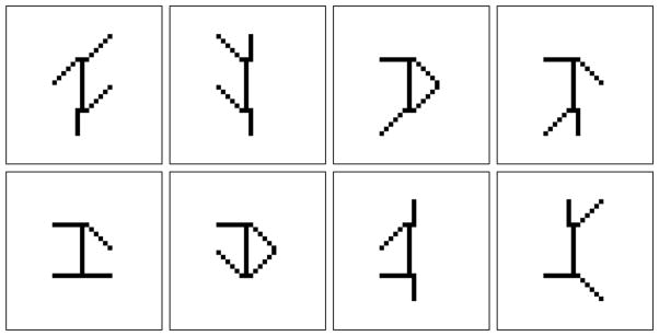
In order to study the effect of the correlated noise on the algorithm we have constructed such noise, where a small part of the image is spatially correlated. Figure 2 shows several random samples from the swimmer dataset of Figure 1 contaminated by the correlated noise.

Fig. 2.

Random samples from the swimmer dataset contaminated by correlated noise. Note the salient spatial correlation with the shape of the swimmer’s torso to the left of the swimmer.

The LS objective function of (3) can be derived from the Gaussian likelihood with noise covariance of the form σ²I. Note that correlated noise results in a differently structured covariance matrix. The covariance of the correlated noise is shown in Figure 3. It is clearly very close to a diagonal matrix. For comparison, the figure also shows a close up image of a section of the covariance, where there are correlations. Correlations among the 2% of the image pixels are high as demonstrated by the high contrast of the covariance image in the figure. Several samples of the noise are shown in Figure 4. The correlated part has the shape of the swimmer’s torso shifted to the left of the original torso position. In summary the noise is mostly white, with a small locally concentrated correlated component.

Fig. 3.

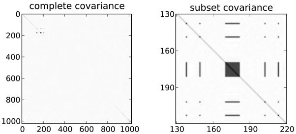
Noise covariance for all 1024 image pixels shows the expected spatial correlations. The covariance is very close to identity, only the 90 by 90 close up on the right shows the correlated part. Such a covariance matrix is favorable to the conventional least squares analysis because it satisfies the assumptions of the method.

Fig. 4.

Correlated noise samples that were added to the swimmer dataset. Note the salient spatial correlation.

A reasonable expectation of NMF’s behavior on this dataset would be a result that has the correlation torso as a separate feature with the other features correctly recovered. This common-sense behavior would go along with other matrix factorization techniques such as independent component analysis (ICA), which exploit this feature for denoising. Surprisingly, we have observed quite different behavior. A typical result is shown in Figure 5, where it becomes clear that correlated noise affects the estimation of all of the features, in addition to being estimated as a separate feature. For comparison the correct factorization that is obtained by NMF from the noiseless dataset is shown in Figure 6. Note that we have observed similar behavior even when using the KL divergence based NMF objective, although we do not pursue this finding further in this work.

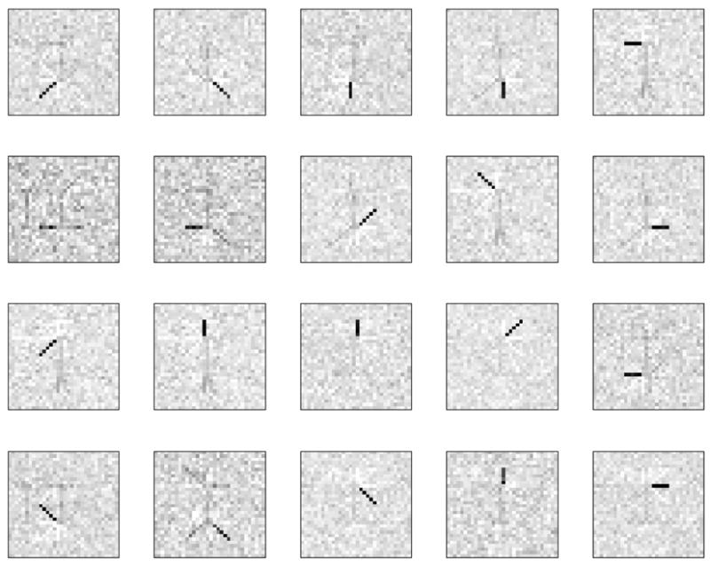
Fig. 5.

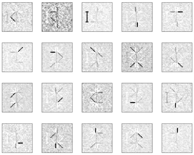
20 features (columns of the W matrix) as extracted by the regular NMF algorithm with the LS objective function from the dataset contaminated by correlated noise.

Fig. 6.

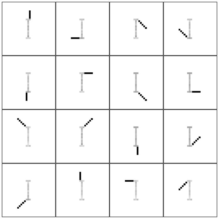
Features extracted by NMF from the noiseless swimmer dataset. Only 16 unique features are shown.

Introduction of the torso-shaped correlation in the noise violates the separability condition from [6]. The condition requires that each part/articulation pair’s presence or absence in the image is indicated by a certain pixel associated to that pair. However, the torso-shaped correlation, when present, can overlap with limbs in some positions. Note that conditions of generative model and complete factorial sampling are still satisfied, because the correlation can always be treated as a separate feature.

4 Proposed Solution

We argue that in practical applications of NMF one needs to model the noise adequately. Here we propose an NMF algorithm that alleviates the problem caused by the correlated noise.

One of the objective functions for non-negative matrix factorization proposed in [1] is the least squares error (LSE) of (3). After rewriting (3) in the matrix form:

$$E=\frac{1}{2}\text{Tr}({(\mathit{X}-\mathit{WH})}^T(\mathit{X}-\mathit{WH})),$$ (10)

the assumption of zero mean noise with unit standard deviation becomes explicit.

For optimization purposes, the formulation is also valid for noise with covariance structure σ²I. Richer noise structures, including those with diagonal covariance or correlated noise, are not captured by such a formulation. The former problem has been addressed in [7]. In this case the scaling of each dimension by a corresponding positive variance is performed. Scaling by the positive constants does not alter the original formulation of multiplicative updates.

We address the problem of generalized least squares (GLS) of (11), where C is the noise covariance, and derive multiplicative updates for this general form of the objective:

$$E=\frac{1}{2}\text{Tr}({(\mathit{X}-\mathit{WH})}^T{\mathit{C}}^{-1}(\mathit{X}-\mathit{WH}))$$ (11)

4.1 Derivation of the updates

To simplify the notation, we define the precision matrix, S = C⁻¹. First, we rewrite the objective:

$$E=\frac{1}{2}(\text{Tr}({\mathit{X}}^T\mathit{SX})+\text{Tr}({\mathit{H}}^T{\mathit{W}}^T\mathit{SWH})-\text{Tr}({\mathit{X}}^T\mathit{SWH})-\text{Tr}({\mathit{H}}^T{\mathit{W}}^T\mathit{SX})).$$ (12)

Then find the derivatives:

$$\frac{\partial E}{\partial \mathit{W}}=\mathit{S}(\mathit{WH}{\mathit{H}}^T-\mathit{X}{\mathit{H}}^T)$$ (13)

$$\frac{\partial E}{\partial \mathit{H}}={\mathit{W}}^T\mathit{S}(\mathit{WH}-\mathit{X}),$$ (14)

where we have used the fact that S is symmetric. Next, we follow the procedure similar to the one used to obtain the updates for the original NMF algorithm [1]. We set the values of the learning rate for both matrices W and H such that the updates become multiplicative. A detailed convergence proof that lead to these values is presented in Appendix. Finally, we arrive at the following multiplicative updates for the GLS error function:

$$\mathit{W}=\mathit{W}\odot \frac{{\mathit{S}}^{+}\mathit{X}{\mathit{H}}^T+{\mathit{S}}^{-}\mathit{WH}{\mathit{H}}^T}{{\mathit{S}}^{-}\mathit{X}{\mathit{H}}^T+{\mathit{S}}^{+}\mathit{WH}{\mathit{H}}^T}$$ (15)

$$\mathit{H}=\mathit{H}\odot \frac{{\mathit{W}}^T{\mathit{S}}^{+}\mathit{X}+{\mathit{W}}^T{\mathit{S}}^{-}\mathit{WH}}{{\mathit{W}}^T{\mathit{S}}^{-}\mathit{X}+{\mathit{W}}^T{\mathit{S}}^{+}\mathit{WH}}$$ (16)

In these updates, the precision matrix is split into two parts as follows:

$$\begin{array}{l}{S}_{ij}^{+}=\{\begin{array}{ll}{S}_{ij}\hfill & S_{ij}>0,\hfill \\ S_{ij}+\lambda \hfill & i=j,\hfill \\ 0\hfill & \text{otherwise},\hfill \end{array}\\ S_{ij}^{-}=\{\begin{array}{ll}\mid S_{ij}\mid \hfill & S_{ij}<0,\hfill \\ \mid S_{ij}\mid +\lambda \hfill & i=j,\hfill \\ 0\hfill & \text{otherwise}.\hfill \end{array}\end{array}$$

In the matrix representation the split of S is expressed as:

$$\begin{array}{l}{\mathit{S}}^{+}={\widehat{\mathit{S}}}^{+}+\lambda \mathit{I}\\ {\mathit{S}}^{-}={\widehat{\mathit{S}}}^{-}+\lambda \mathit{I}\\ \mathit{S}={\widehat{\mathit{S}}}^{+}-{\widehat{\mathit{S}}}^{-}\end{array}$$

where λ is the minimal negative eigenvalue of Ŝ⁻ or 0 if Ŝ⁻ is positive semidefinite or empty. This ensures that S⁻ is positive semidefinite – a condition required for convergence properties of the updates. We defer the proof to the appendix. The appendix also provides details of implementing a projected gradient algorithm for glsNMF.

4.2 Complexity

Introduction of S⁺ and S⁻ added complexity to the updates, namely, four additional matrix multiplications and two matrix summations. Repeating parts of expressions in the numerator and the denominator of equations (16) and (15) can be precomputed before each respective updates. After that only multiplications by parts of the precision matrix and summation of the result are required.

4.3 Covariance estimation

In order for glsNMF to function properly, a good estimate of the noise covariance is required. This is sometimes possible to obtain as a sample covariance of the background measurements of the system without the task of interest. When such background noise is available, it is possible to estimate the covariance using the sample covariance estimation [8]. This is the method we use in this paper. This is especially true in functional electromagnetic brain imaging (an area of increasing use of NMF [4]), where sampling rates allow collection of sufficient samples at least for spatial only analysis. Many models that use the covariance matrix, like glsNMF, assume that it is computed elsewhere.

5 Results

The glsNMF algorithm was applied to the previously introduces noisy swimmer dataset. As before, the number of features was set to 20.

The features obtained by glsNMF are shown in Figure 7. Compare with the features typically obtained by NMF in Figure 5. Note that we have run both algorithms many times changing the starting point. The starting points in the figures are the same.

Fig. 7.

20 features extracted from the noisy dataset by glsNMF.

NMF applied to the noisy dataset produces features spanning several swimmer configurations at once. Thus, it is hard to identify the original noise free image. In addition to that there is a spurious feature – the correlated part of the noise. It is not only present as a feature by itself but also contaminates some other features extracted by the algorithm.

Features extracted by glsNMF are sparse and completely recover the limbs. Furthermore, the correlated part of the noise is not present as a separate feature or as a part of any other features. Although some residual noise still remains even after convergence it does not destroy the parts based representation.

6 Discussion

We have shown that NMF can fail in the case of data contaminated by correlated noise. This is almost always unavoidable situation when dealing with experimental datasets. Issue of noise has been previously addressed in NMF algorithms by rescaling each of the estimates by the amount of noise variance (uncertainty) [7], or by using Gaussian process priors to smooth out the estimates [9]. Results similar to [7] can probably be achieved using the advances in research on weighted NMF [10]. An approach that has formulation similar to our suggested solution was presented in [11]. However, there the goal was not to target correlated noise and also the novelty of our formulation is the multiplicative updates and their convergence proof. In fact, a solution by a projected gradient [12] method is easily possible and we have also derived it for our method including the derivation in Appendix.

There are a multitude of extensions to NMF, such as additional sparsity, convolutive algorithm etc. [13–15]. We believe some of them can benefit from using GLS objective function.

7 Conclusions

A growing interest in application of NMF to experimental datasets [3,4,2,5] requires special handling of issues introduces by unavoidable presence of noise. We have demonstrated that the NMF algorithm can fail in the presence of correlated noise which can violate the separability assumption of unique factorization and degrade the results in applications such as feature extraction. We also proposed the glsNMF algorithm as a solution to the correlated noise problem which is able to recover features from data with correlated noise. For this we have derived a multiplicative update and presented a convergence proof. Our future work includes application of the method to functional brain imaging and gene expression datasets as well as extending the method to deal with large dimensionality of the input space which makes the covariance matrix hard to handle. It is also possible to perform glsNMF with simultaneous estimation of the covariance matrix which we also leave for future work.

Appendix

Convergence proof

Consider the problem for a single column of H denoted by h. The corresponding column of X is given by x. The objective is now given by:

$$F(\mathit{h})=\frac{1}{2}{(\mathit{x}-\mathit{Wh})}^T\mathit{S}(\mathit{x}-\mathit{Wh})$$ (17)

We define an auxiliary function G(h, v) with the properties that G(h, h) = F(h) and G(h, h^t) ≥ F(h), where h^k is the current estimate with iteration index k and h is the free parameter. The multiplicative update rule is found at each iteration by minimizing the auxiliary function:

$${\mathit{h}}^{k+1}=arg\underset{\mathit{h}}{min}G(\mathit{h},{\mathit{h}}^k)$$ (18)

Note that this does not increase the objective function F, as we have

$$F({\mathit{h}}^{k+1})\le G({\mathit{h}}^{k+1},{\mathit{h}}^k)\le G({\mathit{h}}^k,{\mathit{h}}^k)=F({\mathit{h}}^k)$$ (19)

Define G as follows:

$$G(\mathit{h},{\mathit{h}}^k)=F({\mathit{h}}^k)+{(\mathit{h}-{\mathit{h}}^k)}^T\mathbf{\nabla }F({\mathit{h}}^k)+\frac{1}{2}{(\mathit{h}-{\mathit{h}}^k)}^T\mathit{K}({\mathit{h}}^k)(\mathit{h}-{\mathit{h}}^k)$$ (20)

where the diagonal matrix K(h^k) is defined as

$${\mathit{K}}_{ab}({\mathit{h}}^k)={\delta }_{ab}\frac{{({\mathit{W}}^T{\mathit{S}}^{+}\mathit{W}{\mathit{h}}^k+{\mathit{W}}^T{\mathit{S}}^{-}\mathit{x})}_a}{{\mathit{h}}_a^k},$$ (21)

where a and b are indices of vector and matrix elements, and

$${\delta }_{ab}=\{\begin{array}{ll}1,\hfill & \text{if}a=b\hfill \\ 0,\hfill & \text{if}a\ne b\hfill \end{array}$$ (22)

It trivially holds that G(h, h) = F(h). For G(h, h^k) ≥ F(h) to hold we need

$${(\mathit{h}-{\mathit{h}}^k)}^T[\mathit{K}({\mathit{h}}^k)-{\mathit{W}}^T\mathit{SW}](\mathit{h}-{\mathit{h}}^k)\ge 0$$ (23)

We denote M = K(h^k)−W^T SW, observing that M must be positive semidefinite for (23) to hold, and split it into parts as follows:

$$\mathit{M}={\mathit{P}}_1+{\mathit{P}}_2+{\mathit{P}}_3$$ (24)

$${({\mathit{P}}_1)}_{ab}={\delta }_{ab}\frac{{({\mathit{W}}^T{\mathit{S}}^{+}\mathit{W}{\mathit{h}}^k)}_a}{{\mathit{h}}_a^k}-{({\mathit{W}}^T{\mathit{S}}^{+}\mathit{W})}_{ab}$$ (25)

$${({\mathit{P}}_2)}_{ab}={\delta }_{ab}\frac{{({\mathit{W}}^T{\mathit{S}}^{-}\mathit{x})}_a}{{\mathit{h}}_a^k}$$ (26)

$${({\mathit{P}}_3)}_{ab}={({\mathit{W}}^T{\mathit{S}}^{-}\mathit{W})}_{ab}$$ (27)

If each P_i is positive semidefinite then their sum M is also so. The most difficult is P₁ and we show it is positive semidefinite the last. P₂ is trivially positive semidefinite since it is a diagonal matrix with non-negative entries. P₃ is also positive semidefinite since by construction in Section 4.1 we obtain a positive semidefinite S⁻ which can be written as a square root LL^T giving a positive semidefinite P₃ = (W^TL)(W^TL)^T.

We show P₁ to be positive semidefinite using the proof structure of [1] which is as follows:

$${\mathit{Q}}_{ab}({\mathit{h}}^k)={\mathit{h}}_a^k{({\mathit{P}}_1)}_{ab}{\mathit{h}}_b^k$$ (28)

$$\begin{array}{rl}{\mathit{\nu }}^T\mathit{Q}\mathit{\nu }& =\sum _{ab}{\mathit{\nu }}_a{\mathit{Q}}_{ab}{\mathit{\nu }}_b\\ & =\sum _{ab}{({\mathit{W}}^T{\mathit{S}}^{+}\mathit{W})}_{ab}{\mathit{h}}_a^k{\mathit{h}}_b^k[\frac{1}{2}{\mathit{\nu }}_a^2+\frac{1}{2}{\mathit{\nu }}_b^2-{\mathit{\nu }}_a{\mathit{\nu }}_b]\\ & =\frac{1}{2}\sum _{ab}{({\mathit{W}}^T{\mathit{S}}^{+}\mathit{W})}_{ab}{\mathit{h}}_a^k{\mathit{h}}_b^k{({\mathit{\nu }}_a-{\mathit{\nu }}_b)}^2\\ & \ge 0\end{array}$$ (29)

Setting the gradient of G to zero, we obtain an expression for the minimum of G.

$$\mathit{\Delta }=\frac{{\mathit{h}}^k}{({\mathit{W}}^T\mathit{S}+\mathit{W}{\mathit{h}}^k+{\mathit{W}}^T\mathit{S}-\mathit{x})}\odot ({\mathit{W}}^T\mathit{S}(\mathit{W}{\mathit{h}}^k-\mathit{x}))$$ (30)

$$\begin{array}{rl}{\mathit{h}}^{k+1}& ={\mathit{h}}^k-\mathit{\Delta }\\ & ={\mathit{h}}^k\odot \frac{{\mathit{W}}^T{\mathit{S}}^{+}\mathit{x}+{\mathit{W}}^T{\mathit{S}}^{-}\mathit{W}{\mathit{h}}^k}{{\mathit{W}}^T{\mathit{S}}^{-}\mathit{x}+{\mathit{W}}^T{\mathit{S}}^{+}\mathit{Wh}}\end{array}$$ (31)

This is the update rule for h and similarly we can derive the update rule for w.

Projected gradient

To implement a projected gradient solver for glsNMF we require a modification of the original NMF algorithm [12] that accounts for including the covariance into the Gaussian likelihood objective. Individual objectives for W and H written in the vector form vec(·) (columns of a matrix stacked in a vector) are:

$$E_{\mathit{W}}=\mathit{vec}({\mathit{W}}^T)\left(\mathit{H}{\mathit{H}}^T\otimes \mathit{S}\right)\mathit{vec}(\mathit{W})+{\mathit{W}}^{’}\text{s}\text{linear}\text{terms}$$ (32)

$$E_{\mathit{H}}=\mathit{vec}{(\mathit{H})}^T\left(\mathit{I}\otimes {\mathit{W}}^T\mathit{SW}\right)\mathit{vec}(\mathit{H})+{\mathit{H}}^{’}\text{s}\text{linear}\text{terms},$$ (33)

where ⊗ is the Kronecker product defined as

$$\mathit{A}\otimes \mathit{B}=\left[\begin{array}{ccc}{a}_{11}\mathit{B}& \cdots & a_{1n}\mathit{B}\\ ⋮& \ddots & ⋮\\ a_{m1}\mathit{B}& \cdots & a_{mn}\mathit{B}\end{array}\right]$$ (34)

Hessian matrices in both cases tend to be well conditioned when number of training examples is larger than number of features and dimensionality of the data, and S is well conditioned too. The first is a usual case in the application domain of NMF. The second requires a well conditioned sample covariance, which can be provided by estimation from a sufficient population of noise or adequately modeled.

Equation (33) is structurally equivalent to the one presented by Lin [12]. The original routine for solving the subproblem of taking a step in the direction opposite to the maximal gradient ∇_Hf(W, H) can be used with a single change: W^T SW needs to be precomputed instead of the plain W^T W.

A different situation arises in the case of (32). The subroutine of H cannot be used directly and a straightforward solution is to have individual subroutines for H and W. The sufficient decrease test [12, equation 4.3] becomes:

$$(1-\sigma )\langle {\nabla }_{\mathit{W}}f(\mathit{W},\mathit{H}),d\mathit{W}\rangle +\frac{1}{2}\langle d\mathit{W},\mathit{S}d\mathit{WH}{\mathit{H}}^T\rangle \le 0,$$

where 〈·, ·〉 is the sum of element-wise product of two matrices.

The shape of the second term in the sum is derived from the full tensor product of the Hessian with vec (dW) taking advantage of the following identity [16]:

$$\mathit{vec}(\mathit{AXB})=\left({\mathit{B}}^T\otimes \mathit{A}\right)\mathit{vec}(\mathit{X})$$ (35)

The additional complexity with respect to the original projected gradient algorithm for NMF is the matrix multiplication by S. In practice we have found this not be an issue and projected gradient was considerably faster than multiplicative updates, which aligns well with what has been previously observed for NMF.

References

- 1.Lee Daniel D, Seung Sebastian H. Algorithms for non-negative matrix factorization. NIPS. 2000:556–562. [Google Scholar]
- 2.Lohmann Gabriele, Volz Kirsten G, Ullsperger Markus. Using non-negative matrix factorization for single-trial analysis of fMRI data. Neuroimage. 2007;37(4):1148–60. doi: 10.1016/j.neuroimage.2007.05.031. [DOI] [PubMed] [Google Scholar]
- 3.Potluru VK, Calhoun VD. Group learning using contrast NMF: Application to functional and structural MRI of schizophrenia. Circuits and Systems, 2008. ISCAS 2008. IEEE International Symposium; May 2008.pp. 1336–1339. [Google Scholar]
- 4.Mørup M, Hansen LK, Arnfred SM. ERPWAVELAB a toolbox for multi-channel analysis of time-frequency transformed event related potentials. Journal of Neuroscience Methods. 2007;161:361–368. doi: 10.1016/j.jneumeth.2006.11.008. [DOI] [PubMed] [Google Scholar]
- 5.Devarajan Karthik. Nonnegative matrix factorization: An analytical and interpretive tool in computational biology. PLoS Comput Biol. 2008 Jul;4(7):e1000029. doi: 10.1371/journal.pcbi.1000029. [DOI] [PMC free article] [PubMed] [Google Scholar]
- 6.Donoho David, Stodden Victoria. When does non-negative matrix factorization give a correct decomposition into parts? In: Thrun Sebastian, Saul Lawrence, Schölkopf Bernhard., editors. Advances in Neural Information Processing Systems. Vol. 16. MIT Press; Cambridge, MA: 2004. [Google Scholar]
- 7.Wang G, Kossenkov AV, Ochs MF. LS-NMF: a modified non-negative matrix factorization algorithm utilizing uncertainty estimates. BMC Bioinformatics. 2006;7 doi: 10.1186/1471-2105-7-175. [DOI] [PMC free article] [PubMed] [Google Scholar]
- 8.Stark H, Woods JW. Probability and random processes with applications to signal processing. Prentice Hall; Upper Saddle River, NJ: 2002. [Google Scholar]
- 9.Schmidt Mikkel N, Laurberg Hans. Nonnegative matrix factorization with Gaussian process priors. Computational intelligence and neuroscience. 2008:361705. doi: 10.1155/2008/361705. [DOI] [PMC free article] [PubMed] [Google Scholar]
- 10.Guillamet D, Vitri J, Schiele B. Introducing a weighted non-negative matrix factorization for image classification. Pattern Recognition Letters. 2003;24(14):2447–2454. [Google Scholar]
- 11.Cichocki Andrzej, Zdunek Rafal. Regularized alternating least squares algorithms for non-negative matrix/tensor factorization. ISNN 07: Proceedings of the 4th international symposium on Neural Networks; Berlin, Heidelberg. Springer-Verlag; 2007. pp. 793–802. [Google Scholar]
- 12.Lin Chih-Jen. Projected gradient methods for nonnegative matrix factorization. Neural Comp. 2007 Oct;19(10):2756–2779. doi: 10.1162/neco.2007.19.10.2756. [DOI] [PubMed] [Google Scholar]
- 13.Hoyer PO. Non-negative sparse coding. Neural Networks for Signal Processing, 2002. Proceedings of the 2002 12th IEEE Workshop on; 2002. pp. 557–565. [Google Scholar]
- 14.Potluru VK, Plis SM, Calhoun VD. Sparse shift-invariant NMF. Image Analysis and Interpretation, 2008. SSIAI 2008. IEEE Southwest Symposium; mar 2008.pp. 69–72. [Google Scholar]
- 15.O‘Grady Paul D, Pearlmutter Barak A. Convolutive non-negative matrix factorisation with a sparseness constraint. Proceedings of the IEEE International Workshop on Machine Learning for Signal Processing (MLSP 2006); Maynooth, Ireland. sep 2006; pp. 427–432. [Google Scholar]
- 16.Petersen KB, Pedersen MS. The matrix cookbook. 2008 Oct; Version 20081110. [Google Scholar]