Comparing connectivity pattern and small-world organization between structural correlation and resting-state networks in healthy adults

Abstract

In recent years, coordinated variations in brain morphology (e.g. volume, thickness, surface area) have been employed as a measure of structural association between brain regions to infer large-scale structural correlation networks (SCN). However, it remains unclear how morphometric correlations relate to functional connectivity between brain regions. Resting-state networks (RSN), derived from coordinated variations in neural activity at rest, have been shown to reflect connectivity between functionally related regions as well as, to some extent, anatomical connectivity between brain regions. Therefore, it is intriguing to investigate similarities between SCN and RSN to help identify how morphometric correlations relate to connections defined by resting-state connectivity. We investigated the similarities in connectivity patterns and small-world organization between SCN, derived from correlations of regional gray matter volume across individuals, and RSN in 36 healthy individuals. The results showed a significant similarity between SCN and RSN (60% for positive connections and 40% for negative connections) that might be explained by shared experience-related functional connectivity underlying both SCN and RSN. Conversely, the small-world parameters of the networks were significantly different, suggesting that SCN topological parameters cannot be regarded as a substitute for topological organization in resting-state networks. While our data suggest that using structural correlation networks can be useful in understanding alterations in structural associations in various brain disorders, it should be noted that a portion of the observed alterations might be explained by factors other than those reflecting resting-state connectivity.

INTRODUCTION

Coordinated variations in brain morphology (e.g. volume, thickness, surface area) have been recently employed as a measure of structural association between brain regions to infer large-scale structural correlation networks (SCN) (Bassett et al., 2008; Bernhardt et al., 2011; Chen et al., 2008, 2011; Fan et al., 2011; Guye et al., 2010; He et al., 2007, 2008, 2009a; He and Evans, 2010; Hosseini et al., 2012a, 2012b; Lerch et al., 2006; Lv et al., 2010; Raj et al., 2010; Sanabria-Diaz et al., 2010; Sun et al., 2012; Wu et al., 2012; Zhou et al., 2011). Alterations in the arrangements of these networks have been associated with normal aging (Chen et al., 2011; Sun et al., 2012; Wu et al., 2012), multiple sclerosis (He et al., 2009a), Alzheimer’s disease (He et al., 2008; Zhou et al., 2011), schizophrenia (Bassett et al., 2008) and epilepsy (Bernhardt et al., 2011; Raj et al., 2010). However, it remains unclear how morphometric correlations relate to actual anatomical and/or functional connectivity between brain regions.

These morphometric correlations might reflect anatomical connectivity, as axonally connected regions are believed to be influenced by common developmental, trophic and maturational effects (Bernhardt et al., 2011; Cheverud, 1984; Wright et al., 1999; Zhang et al., 2000). This idea is supported by a number of studies that suggest consistencies between networks constructed from morphometric correlations of cortical volume, thickness, and surface area data with those constructed from white matter tract-based data (Bernhardt et al., 2008; He et al., 2007; Lerch et al., 2006; Sanabria-Diaz et al., 2010). Further evidence is provided by a recent study that reported 40% similarity between cortical thickness correlations and diffusion tensor imaging (DTI)-derived anatomical networks (Gong et al., 2012).

Alternatively, morphometric correlations might also be influenced by functional connectivity as functional specialization, through practice, skill acquisition and training, can cause changes in underlying anatomy (experience-related plasticity) (Duan et al., 2012; Gaser and Schlaug, 2003a; Halwani et al., 2011; Maguire et al., 2000, 2006; Rykhlevskaia et al., 2008; Sluming et al., 2002). This possibility is supported by neuroimaging evidence showing, for example, increased gray matter volume in motor, auditory and visual-spatial brain regions in professional musicians in response to long-term skill acquisition (Gaser and Schlaug, 2003a, 2003b), enhanced integration of striatal network in chess experts (Duan et al., 2012), increased gray matter density in Broca’s area in orchestra musicians (Sluming et al., 2002), and increased hippocampal gray matter volume in taxi drivers (Maguire et al., 2000, 2006; Woollett and Maguire, 2011).

Resting-state networks (RSN) (Biswal et al., 1995, 2012), derived from coordinated variations in neural activity at rest, have been shown to reflect connectivity between functionally related regions (Biswal et al., 2010; Greicius et al., 2009). Recent data show that resting-state functional connectivity not only reflects functional connectivity mediated by indirect anatomical connections and experience-related functional plasticity, but also represents, to some extent, the underlying anatomical connectivity between brain regions (Damoiseaux and Greicius, 2009; Honey et al., 2009; Luo et al., 2012; Skudlarski et al., 2008; van den Heuvel et al., 2009a). The gold standard for extracting anatomical connectivity involves invasive retrograde/anterograde tract tracing that cannot be done in the living human (Bernhardt et al., 2011). However, a significant agreement has been demonstrated between a majority of common resting-state connections and known anatomical fiber tracts in monkeys (Mantini et al., 2011; Shen et al., 2012). Thus, it is intriguing to investigate similarities between SCN and RSN to help identify how morphometric correlations relate to functional connections defined by resting-state connectivity.

In the present report, we aimed to identify the similarities between SCN, derived from correlations of regional gray matter volume across individuals and RSN in healthy adults. SCN was represented by a set of nodes that correspond to brain regions and a set of edges (connections) that correspond to statistical correlations in gray matter volume between brain regions, across individuals (Hosseini et al., 2012b; He et al., 2007). RSNs were represented by the same set of nodes while their edges were quantified by computing the statistical correlation between time series of different brain regions (Bassett et al., 2012; Buckner et al., 2009; He et al., 2009b; Liao et al., 2010; Tian et al., 2011; van der Heuvel et al., 2009a; Wang et al., 2009a, 2009b). Thresholding the obtained correlation matrices at an absolute threshold results in networks with different numbers of nodes and connections that might influence the network measures and limit interpretation of comparison findings (van Wijk et al., 2010). Therefore, many recent studies involving brain networks binarize the correlation matrices at fixed network densities (number of existing edges to the number of possible edges in the network) and compare the binary networks across a range of densities (Alexander-Bloch et al., 2013; Bassett et al., 2012; Bernhardt et al., 2011; Bruno et al., 2012; Fan et al., 2011; He et al., 2009a; Hosseini et al., 2012a, 2012b; Sanabria-Diaz et al., 2010; Wang et al., 2010; Wu et al., 2012).

Similarities between two networks can be assessed by either comparing the similarity of their connections or by comparing their organizational properties. The most direct way of comparing connections in networks with the same size is to find their distances. The distances between two binary networks are usually calculated using the Hamming distance (S_hd), which measures the number of addition/deletion operations required to make two networks the same (van Wijk et al., 2010). While Hamming distance gives an accurate estimate of similarity between network connections, it overestimates the similarity if the networks are sparse (Fig. 1). Therefore, we also used a normalized distance metric (S_norm) that accounts for large baseline correlations between networks (Costa et al., 2007).

Figure 1. Network comparison.

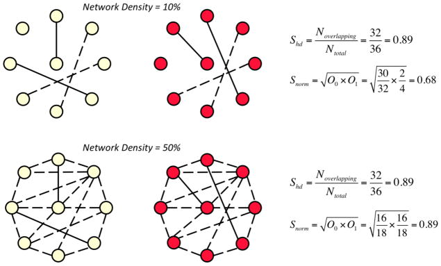
An illustrative example on how S_hd and S_norm differ in measuring similarities between sparse and dense networks. Top panel shows two example networks at density of 10%. There are two overlapping and two divergent connections between networks (out of four connections). Since the networks are sparse, S_hd gives 89% similarity between networks (most of which arise from shared disconnections) while S_norm only gives 68% similarity. Bottom panel shows two networks at 50% density. These networks were constructed by adding additional 14 overlapping connections to the top networks. Thus, they have 16 overlapping and two divergent connections (out of 18 connections). Adding 14 overlapping connections to the networks does not change S_hd output but increases the S_norm output. Since these networks are not sparse, both S_hd and S_norm gives a similar result for similarity.

We also compared the organizational properties of SCN and RSN to assess their similarities in terms of information processing potential. Previous studies have shown that SCNs and RSNs follow small-world architecture in healthy individuals (Bassett et al., 2008, 2012; He et al., 2009a; Fan et al., 2011; Hosseini et al., 2012a, 2012b, 2013; Wu et al., 2012), an architecture that provides optimal balance between local and global information processing in the network (Amaral et al., 2000; Bassett and Bullmore, 2006; Latora and Marchiori, 2001; Watts and Strogatz, 1998). Therefore, we compared the organizational properties of SCN and RSN by directly measuring their small-world characteristics at the global level as well as their connectedness properties at the regional level.

A recent study by Alexander-Bloch and colleagues (2013) examined the convergence of SCN constructed from cortical thickness data and RSN in healthy individuals and reported a significant correlation between the two networks (Alexander-Bloch et al., 2013). However, they constructed SCN for cortical thickness data and did not include the subcortical regions. In the present study, we used regional volume data to construct SCN since they contain information regarding both thickness and surface area and thus reflect a summary effect of interaction between brain regions. Using regional volume data also allowed us to compare SCN and RSN networks that includes both cortical and subcortical regions. In addition, the current study expands the previous findings by comparing the similarities and small-world indices between SCN and RSN across a large range of density thresholds. Finally, we tested the reproducibility of our findings by comparing RSN and SCN networks of the same subjects across two time points.

We expected a degree of similarity between SCN and RSN that might be explained by the shared influence of both anatomical connectivity and experience-related plasticity. We also expected a higher small-world index in RSN compared to SCN since functional networks require rapid transitions and reconfigurations and would allow higher rates of information processing.

MATERIALS AND METHODS

Participants

We enrolled 36 healthy adults (age 20 – 39 years old, mean age 28.4) in the study (Table 1). Participants were excluded for any history of medical, neurologic or psychiatric conditions or MRI contraindications. The Stanford University Institutional Review Board approved the study. This study was conducted according to the principles expressed in the Declaration of Helsinki. All participants provided written informed consent.

Table 1.

Demographics of the participants

N	36
Age (years)	28.4 (4.65)
Education (years)	17 (2.72)
Gender	19F, 17M
Ethnicity	3A, 5B, 1PI, 27W

F: female; M: males; A: Asian; B: Black; PI: Pacific Islander; W: White

MRI data acquisition

MRI scanning was performed on a GE Discovery MR750 3.0 Tesla whole body scanner (GE Medical Systems, Milwaukee, WI). High-resolution T1-weighted images were acquired with 3D spoiled gradient recall pulse sequence using the following parameters: TR = 8.5ms, TE = 3.396, TI = 400 ms, flip angle = 15°, FOV = 220 mm, number of excitation =1, acquisition matrix = 256 × 192, slice thickness = 1.6. Totally, 124 contiguous coronal slices were obtained with in-plane resolution of 0.859 mm × 0.859 mm. Resting-state functional MRI data was acquired, in the same session, while participants rested in the scanner with their eyes closed using a T2* weighted gradient echo spiral pulse sequence: relaxation time = 2000 msec, echo time = 30 msec, flip angle = 80° and 1 interleave, field of view = 220 mm, slice thickness = 4 mm, spacing = 1 mm, matrix = 64×64, in-plane resolution = 3.125. Number of data frames collected was 216 with a total scan time of 7:12 min. An automated high-order shimming method based on spiral acquisitions was employed to reduce field heterogeneity (Glover and Lai, 1998).

Image preprocessing

Anatomical image preprocessing was performed using Statistical Parametric Mapping 8 (SPM8; Wellcome Department of Cognitive Neurology, London, UK) (Friston, 2007) as described in detail in our previous publications (Hosseini et al., 2012a, 2012b). The anatomical images were segmented into gray matter (GM), white matter, and cerebrospinal fluid images based on the ICBM Tissue Probabilistic Maps (http://www.loni.ucla.edu/ICBM/ICBMTissueProb.html). A study-specific a priori probability map of GM was created from the modulated spatially normalized segmented GM images using the Template-O-Matic (TOM8) toolbox (Wilke et al., 2008). Custom priors were then affine-registered to the standard Montreal Neurological Institute space. Voxel-based morphometry (VBM) analysis was performed using the VBM8 toolbox for SPM8 (http://dbm.neuro.uni-jena.de/vbm), which involved 1) segmentation of MR images into GM tissue segments, 2) non-linearly warping the tissue segments to the GM study-specific customized template model (Ashburner and Friston, 2005), and 3) modulation of the normalized images to ensure that relative volumes of GM were preserved following the spatial normalization procedure. Sample homogeneity was examined to identify any outliers in the study population. Images were visually inspected for correct spatial normalization, and the VBM toolbox was used to semi-automatically check for inhomogeneities. Images were also inspected for artifacts and structural abnormalities. No images required exclusion.

It should be noted that cortical volume is the product of cortical thickness and surface area. While each of these measures reflects distinct genetic, developmental and biological processes, the volume measure conflates all of these effects. On the other hand, VBM-based measure of gray matter volume may be contaminated by registration bias and partial volume effects (Bookstein 2001, Ashburner and Friston 2001). However, previous studies on volumetric covariance networks, including our own, have shown that the obtained network parameters are highly consistent with those derived using thickness covariance networks (Bassett et al., 2008; Hosseini et al., 2012a, 2012b; Fan et al., 2011; Wu et al., 2012).

There are various nodal definition methods in brain network analysis. While the results might be affected by the choice of parcellation scheme, recent evidence indicates that the results of between-network comparison remain intact regardless of the applied parcellation scheme (Zalesky et al., 2010). We generated 90 cortical and subcortical regions of interest (ROIs), excluding the cerebellum, from the Automated Anatomical Labeling (AAL) atlas using the WFU PickAtlas Toolbox (Tzourio-Mazoyer et al., 2002). AAL does not offer a parcellation where individual regions are comparable in size (or area) and may thus blur connectional patterns of smaller subregions within the bigger ROIs (Zalesky et al., 2010). However, most of the previous graph analysis studies of structural and functional correlation networks have successfully employed this parcellation scheme (Achard and Bullmore, 2007; Achard et al., 2006; Bassett et al., 2012; Fan et al., 2011; He et al., 2009b; Hosseini et al., 2012a, 2012b; Lynall et al., 2010; Meunier et al., 2009; Sanz-Arigita et al., 2010; Supekar et al., 2008, 2009; Wang et al., 2009b; Wu et al., 2012; Zhang et al., 2011). We used AAL to keep our results consistent with the current studies. These AAL ROIs were resliced to the same dimension as that of tissue segmented images obtained from the VBM preprocessing step. The ROIs were subsequently used to mask the individual modulated, normalized GM images and extract the average volume within each ROI using the REX toolbox (http://web.mit.edu/swg/software.htm). A linear regression analysis was performed at every ROI to remove the effects of total brain volume. The residuals of this regression were then substituted for the raw ROI volume values (Bernhardt et al., 2011; Fan et al., 2011; He et al., 2007; Hosseini et al., 2012a, 2012b) and are referred to as corrected regional gray matter volumes (RGV), hereafter.

Functional MRI preprocessing was also performed using SPM8 as described in our previous publications (Kesler et al., 2009, 2011). In summary, images were first realigned to correct for head motion. The realigned images were then coregistered and normalized using the segmented anatomical volume. Images were visually assessed for correct spatial normalization. We utilized the same AAL atlas (90 regions representing cortical and subcortical structures in both hemispheres) as mentioned in the previous section. The ROIs were identical to those used in previous graph analysis studies of the functional connectome (Achard and Bullmore, 2007; Achard et al., 2006; Bassett et al., 2012; He et al., 2009b; Lynall et al., 2010; Meunier et al., 2009; Sanz-Arigita et al., 2010; Supekar et al., 2008, 2009; Wang et al., 2009b; Zhang et al., 2011). Further processing of the functional volumes was performed using the Functional Connectivity Toolbox (http://web.mit.edu/swg/software.html) (Whitfield-Gabrieli and Nieto-Castanon, 2012) as described in our previous publication (Bruno et al., 2012). First, data were band pass filtered to 0.008 Hz – 0.09 Hz. Then, the CompCor method was used to reduce physiological and other noise artifacts (Behzadi et al., 2007). This method involves extracting signal from white matter and cerebrospinal fluid (CSF) regions using principal component analysis and then regressing these signals out of the total fMRI signal. The individual motion parameters (output from realignment) were also used as covariates. Recently, Schwartz and McGonigle (2011) compared organization of functional brain networks with and without correction for global signal and showed that deconvolution of white matter, CSF and motion (without removing global signal) resulted in the most robust within-subject reproducibility of global network parameters. In addition, compared to methods that rely on global signal regression, the CompCor noise reduction method allows for interpretation of anticorrelations as there is no regression of the global signal (Whitfield-Gabrieli and Nieto-Castanon, 2012). Finally, temporal correlations between all possible pairs of regions were computed based on the corrected fMRI signal resulting in a 90×90 correlation matrix r_f for each participant.

Network construction

SCN was constructed at the group level. A 90 × 90 association matrix R_s was generated by performing Pearson correlation coefficient between the corrected RGV across subjects (Bernhardt et al., 2011; Chen et al., 2008, 2011; Fan et al., 2011; He et al., 2007, 2009a; Hosseini et al., 2012a, 2012b). An alternative measure for inferring connectivity is partial correlation that attempts to remove the effect of indirect paths (Smith et al., 2011). However, partial correlation is not suitable for studies with a sample size smaller than the number of ROIs (Zalesky et al., 2012).

Previous studies have shown that the structural and functional correlation networks are estimable with tens of subjects and the small-world results are consistent with those obtained using larger sample size (Bruno et al., 2012; Fan et al., 2011; Hosseini et al., 2012a, 2012b; van den Heuvel et al., 2009b). However, in order to demonstrate the reproducibility of the results with larger sample size, we combined the current data with the prospective resting state and structural data of the same set of subjects (scanned approximately six weeks after the first acquisition). Half of the subjects underwent an active online cognitive training during this period. Since we are comparing the SCN and RSN networks for the same subjects, combining the longitudinal data is helpful as confirmatory analysis. However, the correlation results may have been slightly inflated by the use of longitudinal data. Therefore these results are provided as supplementary to our main analysis. To test the reproducibility of the results, we performed an additional analysis and compared the similarity indices for networks constructed at each time point, separately. To this purpose, the same similarity analyses were performed on networks constructed from the second time point data. Then, Spearman correlation was used to examine the correlation between similarity indices (obtained at the same range of network densities) across time points.

Unlike SCNs that are constructed at the group-level, RSNs are computed at the individual-level. In order to directly compare the SCN and RSNs, the individual correlation matrices obtained from functional connectivity analysis (r_f) were first converted to z-score matrices using Fisher’s r-to-z transformation. We then averaged the z-scores across individuals to obtain a group-level z-score matrix Z_f. Finally we converted the mean z-scores back to correlation values to obtain a group-level functional association matrix R_f. The resultant group-level association matrices (R_s and R_f) were used for further constructing SCN and RSN.

The obtained association matrices comprise a set of correlation values ranging from −1 to 1. The majority of previous studies involving structural and functional correlation networks only considered positive correlations as a measure of connectivity (Achard et al., 2006; Bernhardt et al., 2011; Bruno et al., 2012; Fan et al., 2011; He et al., 2007, 2008; Hosseini et al., 2012a, 2012b; Wang et al., 2009a). In this study, we constructed the networks for both positive and negative correlation ranges separately. Specifically, the diagonal elements of the R_s and R_f were first set to zero. Then, to obtain networks of positive correlations (R_s-pos and R_f-pos), all the negative correlations in R_s and R_f were set to zero. Conversely, to obtain negative correlation networks (R_s-pos and R_f-pos), only negative correlations in R_s and R_f were retained and the absolute values of the remaining negative weights were considered for network construction. All the comparisons between SCN and RSN were performed for positive (SCN_pos vs. RSN_pos) and negative (SCN_neg vs. RSN_neg) correlations separately.

Thresholding procedure

As noted above, using an absolute threshold can limit network comparisons. Therefore, we derived binary adjacency matrices A_s-pos, A_s-neg, A_f-pos, A_f-neg by thresholding the association matrices R_s-pos, R_s-neg, R_f-pos, R_f-neg at a range of network densities, respectively (Bernhardt et al., 2011; Bruno et al., 2012; Fan et al., 2011; He et al., 2008; Hosseini et al., 2012b). The obtained adjacency matrices represented binary undirected graphs G_s-pos, G_s-neg, G_f-pos, G_f-neg in which regions i and j were connected if g_ij was equal to 1. The obtained graphs had a network degree of E equal to the number of edges, and a network density (cost) of D =E / [N × (N−1) / 2] representing the ratio of existing edges relative to all possible edges. We thresholded the networks across a range of network densities (0.01: 0.02: D_max). The upper bound D_max was determined as min [max (D_s), max (D_f)], where D_s and D_f represent the density of the thresholded structural and functional networks, respectively. D_max was 0.65 (0.14) for comparing positive (negative) connections.

Small-world parameters

The small-worldness of a complex network, as described in the introduction, has two key metrics: the clustering coefficient C and the characteristic path length L of the network. The clustering coefficient of a node is a measure of the number of edges that exist between its nearest neighbors. The clustering coefficient of a network is thus the average of clustering coefficients across nodes and is a measure of network segregation. The characteristic path length of a network is the average shortest path length between all pairs of nodes in the network and is the most commonly used measure of network integration (Rubinov and Sporns, 2010). To evaluate the topology of the brain network, these parameters must be compared to the corresponding mean values of a benchmark random graph (Maslov and Sneppen, 2002; Milo et al., 2002). The benchmarking random networks were constructed using a rewiring algorithm that preserves the topology of the graphs; i.e. random graphs with the same number of nodes, total edges and degree distribution as the network of interest (Milo et al., 2002; Maslov and Sneppen, 2002; Hosseini et al., 2012b). The small-worldness index of a network is obtained as SW = [C / C_rand] / [L / L_rand] where C_rand and L_rand are the mean clustering coefficient and the characteristic path length of the m = 20 random networks (Bassett and Bullmore, 2006; Hosseini et al., 2012b). In a small-world network, the clustering coefficient is significantly higher than that of random networks (C / C_rand ratio greater than 1) while the characteristic path length is comparable to random networks (L / L_rand ratio close to 1).

The small-world parameters were quantified using the code provided in the Brain Connectivity Toolbox (BCT) described by Rubinov 2010 (Rubinov and Sporns, 2010). The network and statistical analyses were performed using our in-house software, Graph Analysis Toolbox (GAT) (Hosseini et al., 2012b).

Analyzing similarities between SCN and RSN

We employed two metrics in order to assess the similarities between the thresholded binary networks. The first metric examined the ratio of overlapping connections (and disconnections) between networks to the number of all possible connections: S_hd = N_overlapping / N_total. S_hd is 1 when the two networks are the same and is 0 when they are completely opposite (mirrored). While S_hd gives an accurate estimate of similarity between networks, it overestimates the similarity if the networks under consideration are sparse (the number of ones and zeros are significantly different). To overcome this problem, a normalization procedure was proposed to correct for large baseline correlations in sparse binary networks (Costa et al., 2007; van Wijk et al., 2010). This normalized metric assesses the similarity by taking the geometrical average between the ratios of overlapping connections and overlapping disconnections (zeros). For two binary network0s G_s and G_f, the similarity is computed as $S_{\mathit{norm}}=\sqrt{O_0\times O_1}$ where O₁=(number of common connections between G_s and G_f) / (number of total connections in G_s) and O₀=(number of common disconnections between G_s and G_f) / (number of total disconnections in G_f). S_norm equals 1 if two networks are similar and will be zero if they do not have any common connections (or disconnections). We mainly focused on S_norm results as this metric is more appropriate for comparing similarities between networks, regardless of the degree of sparsity.

In order to test the statistical significance of differences in similarity between structural and resting-state networks (G_s vs. G_f), the following procedure was performed: 1000 bootstrap networks were generated for G_s and G_f by random sampling of subjects with replacement and then computing the connectivity matrices separately (BS_s, BS_f). The same bootstrap sampling was used for both G_s and G_f. The similarity measures S_hd and S_norm between BS_s and BS_f networks were quantified. 1000 random networks (SIM_s and SIM_f) were generated with the same density as the bootstrap networks. A 2-sample t-test was used to examine the significance of differences in similarity scores obtained from comparing BS_s and BS_f and those from comparing SIM_s and SIM_f. This procedure was performed separately for positive (G_s-pos vs. G_f-pos) and negative (G_s-neg vs. G_f-neg) correlation networks.

Since comparing the networks at different densities results in multiple comparisons, a summary measure using functional data analysis (FDA) was quantified (Bassett et al., 2012; Hosseini et al., 2012b; Ramsay and Silverman, 2005). In FDA, the similarity score (s) is treated as a function of network density (d) (s = f(d)). The summation of s-values is then calculated at a range of density for BS_s and BS_f as well as for SIM_s and SIM_f networks. Then a 2-sample t-test is used to examine the significance of difference between the observed summary metric of similarity, as described above. We used FDA instead of area-under the curve (AUC) analysis since it is more sensitive to differences in the shape of the curves rather than their mean.

Analyzing similarities between small-world parameters of SCN and RSN

In order to test the statistical significance of the differences in small-world parameters between SCN and RSN, we used the 1000 bootstrap networks generated for structural and resting state networks, described in the previous section. We then computed the small-world parameters (C, L, and SW) for each of these bootstrap networks. A paired t-test was then used to test the significance of differences in small-world parameters between structural and resting-state bootstrap networks. Similar to the comparison of similarity scores, an FDA analysis was performed to compare the summary metrics of small-world parameters at a range of network densities.

Analyzing similarities between regional network properties of SCN and RSN

We performed Spearman’s rank correlation to investigate network similarities in terms of regional topology. Network similarities in FDA of regional clustering coefficient and regional degree were investigated. In addition, we compared the distribution of hubs in SCN and RSN. Hubs are crucial components for efficient communication in a network. They are considered important regulators of information flow and play a key role in network resilience to insult (Rubinov and Sporns, 2010). A node is considered a hub if its regional betweenness centrality is 1 SD higher than the mean network betweenness (Bernhardt et al., 2011). Nodal betweenness centrality is defined as the fraction of all shortest paths in the network that pass through a given node and is used to detect important anatomical/functional connections in the network (Rubinov and Sporns, 2010). Hub analysis was also performed on the summary metric (FDA) of nodal betweenness.

We also investigated the pattern of distribution of regional connectivity (degree distribution) in SCN and RSN. Degree distribution reveals specific characteristics of the network and its resilience to random failure and targeted attacks (Achard et al., 2006; Albert et al., 2000; He et al., 2007). Degree distribution of small-world brain networks has been shown to follow an exponentially truncated power-law distribution (Bassett and Bullmore, 2006; He et al., 2007; Iturria-Medina et al., 2008), formulated as P(d) ~ [d ^(e−1) * exp(−d / d_c)]. P(d) is the probability of network regional degree (d), d_c is the cut-off degree above which there is an exponential decay in probability of hubs and e is the exponent, and indicates a scaling regimen, followed by an exponential decay in the probability of nodes with nodal degree greater than a cutoff value of d_c. We computed the degree distribution for networks thresholded at the minimum density at which both SCN and RSN were not fragmented (d_min = 0.12).

RESULTS

Similarities between SCN and RSN

Positive correlations

Similarities between SCN_pos and RSN_pos as a function of network density are shown in Fig. 2 and Fig. S1. As expected, at lower densities where the networks were sparse, S_hd gave a higher degree of similarity between SCN and RSN (close to 1) (Fig. S1. A) compared with S_norm (around 0.6) (Fig. 2. A). However, at medium network densities, both similarity metrics showed 60% similarity between networks. Both similarity metrics revealed a significant similarity between SCN_pos and RSN_pos (at all densities) when compared with the similarity of randomly simulated networks (p < 10⁻⁶). Additionally, the FDA analysis showed that both S_hd and S_norm was significantly greater for G_s-pos vs. G_f-pos comparison compared with corresponding random networks comparison (p < 10⁻⁶). The localization of connections/disconnections that were similar or different between SCN_pos and RSN_pos is shown in Fig. 3. For demonstration purposes, an illustration of similarity indices across regions is given in Fig. 3. C. A side-by-side comparison of connectivity patterns for a number of seed regions that showed high similarity between networks is also shown in Fig. 4.

Figure 2. Similarities between SCN and RSN bootstrap networks compared with simulated networks as a function of network density.

A) Similarity based on S_norm between SCN_pos and RSN_pos bootstrap networks (BS) (red circles) compared with similarity between equivalent simulated networks (SIM) (black dots) across the density range (0.01: 0.02: 0.65). B) Similarity based on S_norm between SCN_neg and RSN_neg bootstrap networks (BS) (red circles) compared with similarity between equivalent simulated networks (SIM) (black dots) across the density range (0.01: 0.02: 0.14). Dashed lines represent 2SD deviations from the mean similarity. Although the distributions of BS and SIM networks are overlapped for SCN_neg and RSN_neg comparison, they are significantly different (p < 0.05).

Figure 3. Similarities and differences in connectivity between SCN_pos and RSN_pos.

A) A similarity map indicating the connections that are similar (red) or different (black) between SCN_pos and RSN_pos networks, thresholded at an arbitrary density of 33%. Overlapping disconnections are shown in dark blue. For clarity, only regions in the left hemisphere are labeled and the right hemisphere regions are shown immediately below/ to the right of their corresponding left hemisphere regions and left unlabeled. B) The mapping of overlapping connections on brain for left (L) and right (R) hemispheres. C) The localization of similarity indices across brain regions. Connectivity pattern in the occipital, prefrontal and parietal regions showed the highest similarity.

Figure 4. Comparison of connectivity patterns for different seed regions.

The patterns of similarity for three seed regions that showed high similarity between networks are illustrated. The red (yellow) lines represent connections that are common (different) between RSN and SCN. The similarity index for the left MFG, left SMG and right PCC networks was 69%, 75% and 66%, respectively.

Negative correlations

Similarities between SCN_neg and RSN_neg as a function of network density are shown in Fig. 2 and Fig. S1. At lower densities where the networks were sparse, S_hd gave a higher degree of similarity between SCN_neg and RSN_neg (close to 1) (Fig. S1. B) compared with S_norm (around 0.1) (Fig. 2. B). Maximum similarity between SCN_neg and RSN_neg as quantified by S_norm was 40% at 13% density. Both similarity metrics revealed a significant similarity between SCN_neg and RSN_neg when compared with similarity of randomly simulated networks at a range of network densities (Density > 0.05, p < 0.05). Additionally, the FDA analysis showed that both S_hd and S_norm was significantly greater for G_s-pos vs. G_f-pos comparison compared with corresponding random networks comparison (p < 10⁻⁶).

The results of similarity analysis using the combined data, as well as for the second time point data, were consistent with the above observations for positive and negative networks (Fig. S3 and S4). In addition, there was a significant correlation between the obtained similarity indices across the two time points (p < 0.0001). For SCN_pos vs. RSN_pos comparison, the correlation between similarities across time points was 0.99 for S_hd and 0.89 for S_norm. For SCN_neg vs. RSN_neg comparison, the correlation between similarities across time points was 0.99 for both S_hd and S_norm.

Similarities between small-world parameters of SCN and RSN

Positive correlations

Small-world parameters of SCN_pos and RSN_pos as a function of network density are shown in Fig. 5. The normalized clustering coefficient and characteristic path length were significantly greater in RSN_pos than in SCN_pos resulting in a significantly greater small-world index in RSN_pos across a range of network densities (all p’s < 10⁻⁶). The FDA analysis confirmed these results and showed significantly greater small-world parameters in RSN_pos than in SCN_pos (p < 10⁻⁶).

Figure 5. Changes in small-world properties of bootstrap networks for SCN_pos and RSN_pos as a function of network density.

A) normalized path length, B) normalized clustering and C) small-world index for SCN_pos bootstrap networks (BS-S) (black circles) and RSN_pos bootstrap networks (BS-F) (blue squares) across the density range (0.01: 0.02: 0.65). Both networks follow a small-world organization. However, the estimated small-world parameters were significantly different between networks.

Negative correlations

Small-world parameters of SCN_neg and RSN_neg as a function of network density are shown in Fig. S2. The results showed that negative correlation networks do not follow small-world architecture across the range of densities (SW < 1). As for positive correlations, the path length was significantly greater in RSN_neg than in SCN_neg at a range of densities (all p’s < 10⁻⁶). Conversely, normalized clustering and small-world index was significantly greater in SCN_neg than in RSN_neg (Density > 0.05, all p’s < 10⁻⁶). The FDA analysis confirmed these results and showed significantly smaller path length and significantly greater clustering and small-world index in RSN_neg than in SCN_neg (p < 10⁻⁶).

Similarities between regional network properties of SCN and RSN

Since we did not observe small-world architecture in SCN_neg and RSN_neg, we only investigated the similarities in regional topological parameters between SCN_pos and RSN_pos. While regional degree of SCN_pos and RSN_pos was significantly correlated (r = 0.332, p = 0.001) (Fig. 6), correlation in regional clustering coefficient between networks was not significant (r = 0.034, p = 0.75). We also quantified the network hubs for SCN_pos and RSN_pos (Table 2). Compared to SCN_pos, RSN_pos showed a larger number of hubs (fourteen vs. nine hubs).

Figure 6. Relationship between regional degree in SCN_pos and RSN_pos.

A significant Spearman rank correlation was found between regional degree in SCN_pos and RSN_pos. Black circles represent brain regions and the red line represents the linear relationship between regional degree in SCN_pos and RSN_pos.

Table 2.

Distribution of hubs in SCN_pos and RSN_pos

SCNpos	RSNpos
L Inferior frontal, orbital part	R Inferior frontal, opercular part
R Superior frontal, orbital part	L Inferior frontal, orbital part
B Insula	B Fusiform
L Lingual gyrus	R Postcentral
R Parahippocampal gyrus	L Rolandinc operculum
B Precuneus	B Inferior temporal gyrus
R Inferior temporal gyrus	B Middle temporal gyrus
	B Superior temporal pole
	B Superior temporal gyrus

R: right, L: left, B: bilateral. Regions highlighted bold indicate hub regions that are common between networks.

Degree distribution in both SCN_pos and RSN_pos networks followed an exponentially truncated power-law distribution (Fig. 7). The exponent estimate (e) was 1.36 for SCN_pos and 1.57 for RSN_pos. The cut-off degree (d_c) was 1.87 for SCN_pos and 1.65 for RSN_pos. The goodness-of-fit value (R-square) was 0.99 for SCN_pos and 0.92 for RSN_pos (R-square value close to 1 represents a perfect fit).

Figure 7. Degree distributions in SCN_neg and RSN_neg.

The log-log plot of cumulative degree distributions in A) SCN_pos and B) RSN_pos thresholded at d_min = 0.12. The solid line indicates the exponentially truncated power-law curve fitted to the cumulative degree distribution of the networks (black circles). The estimated exponent was 1.36 for SCN_pos and 1.57 for RSN_pos, the cut-off degree was 1.87 for SCN_pos and 1.65 for RSN_pos. These parameters resulted in R-square values of 0.99 and 0.92 for SCN_pos and RSN_pos, respectively.

DISCUSSION

In this report, we investigated the similarities between structural correlation networks, derived from correlations of regional gray matter volume, and resting-state networks. While the results showed a significant similarity between SCN and RSN constructed from positive correlations (60% similarity), the small-world properties were significantly different between these networks. Specifically, the small-world index of resting-state network was higher than that of structural correlation networks. Conversely, we observed very low similarity between structural correlation and resting-state networks extracted from negative correlations (10–40% similarity). The organization of these negative networks was randomized and did not show small-world architecture.

Connectivity in SCN vs. RSN

We compared the connectivity between SCN and RSN by investigating the degree of overlapping connections between networks. S_hd and S_norm formulations were used for this purpose.

Positive correlations

The similarity index S_norm revealed 60% similarity between SCN_pos and RSN_pos that was consistent across network densities; suggesting that the normalized similarity index accounts for biases in sparsity threshold. The observed similarity was significant compared with similarity of randomly simulated networks. Similar results were observed for the combined data (72 subjects). This provides some confirmation of our analysis in a larger sample although the correlation may have been slightly inflated by the use of longitudinal data within the same subjects. The results confirmed the recent report that showed a significant correlation between thickness SCN and RSN (Alexander-Bloch et al., 2013). In addition, we found a significant agreement between similarities obtained across two different time points for the same set of subjects that further confirms our findings.

The observed 60% similarity between SCN_pos and RSN_pos suggests a certain degree of convergence between volumetric correlations and resting-state connectivity that is higher than expected by chance. A portion of this similarity is likely driven by anatomical connectivity underlying both structural correlation and resting-state networks. There is a body of evidence that suggest resting-state connectivity reflects underlying anatomical connectivity architecture of the brain. Van der Heuvel and colleagues (2009a) reported that the majority of commonly found resting-state subnetworks (e.g. default-mode network, visual and motor networks, frontoparietal networks) were interconnected by known anatomical white matter tracts. Skudlarski and colleagues (2008) found a significant agreement between resting-state networks and DTI-based anatomical networks. They reported that agreement was high, specifically in regions with strong overall connectivity. Other studies have also shown positive correlation between anatomical connectivity, derived from in-vivo diffusion weighted imaging, and resting-state connectivity (Greicius et al., 2009; Honey et al., 2009).

Additionally, axonally connected regions are believed to be influenced by common developmental and trophic effects (Bernhardt et al., 2011; Cheverud, 1984; Wright et al., 1999; Zhang & Sejnowski, 2000). Lerch and colleagues (2006) reported consistent connectivity patterns seeding from inferior frontal, opercular part between cortical thickness correlation and DTI tractography networks (Lerch et al., 2006). Other studies also reported a degree of similarity between morphometric correlations and known anatomical fiber tracts (Bernhardt et al., 2008; Gong et al., 2012; He et al., 2007). Specifically, Gong and colleagues (2012) have recently investigated the similarity between cortical thickness correlations and DTI-derived anatomical connectivity and reported 40% similarity between these networks. Finally, morphometric associations are also influenced by neurological disorders that involve alterations in anatomical connectivity (Bullmore et al., 1998; Mitelman et al., 2005a). For example, schizophrenia is associated with cortical thinning in frontal-temporal regions (Kuperberg et al., 2003) that further affects the morphometric correlations in these regions (Mitelman et al., 2005b). Consistent with these reports, Alexander-Bloch and colleagues (2013) reported a significant agreement between thickness SCN and maturational correlation networks, constructed from correlation of rate of changes in cortical thickness over 6–12 years of development. They suggested that synchronized pruning of anatomically connected regions during adolescence might drive population covariance in cortical thickness.

Another source of similarity between structural correlation and resting-state networks might be driven by functional connectivity mediated by indirect anatomical connections. RSN connectivity has been demonstrated between regions that have little or no anatomical connectivity [see (Damoiseaux et al., 2009) for a review]. These functional connections appear to be mediated by indirect anatomical connections (through a third region) or by simultaneous elicitation of activities in two regions with no anatomical connections (Honey et al., 2009; Rykhlevskaia et al., 2008). These connections seem to reflect a history of coactivation between brain regions and experience-related functional plasticity. For example, musicians showed a significant increase in resting-state functional connectivity in the motor and multi-sensory cortices compared with non-musicians, suggesting an experience-related functional plasticity in perceptual and motor networks resulting from long-term synchronization of these regions by musical training (Luo et al., 2012).

Morphometric correlations might also arise from functional specialization of certain brain regions through experience-related plasticity. As noted above, previous studies have shown coordinated changes in gray matter structure in various brain regions in response to professional experience (Gaser and Schlaug, 2003a, 2003b; Maguire et al., 2000, 2006). Additionally, several studies have shown changes in cortical morphology in response to short-term intensive training on a specific task, suggesting a possible functional significance of the structural changes (Bezzola et al., 2011; Boyke et al., 2008; Engvig et al., 2010; Hyde et al., 2009a, 2009b). A significant increase in gray matter volume has been observed in novice golf players after 40 hours of golf training in task-relevant cortical network comprising sensorimotor and occipital-parietal regions (Bezzola et al., 2011). Changes in brain deformations in motor regions were also observed after 15 months of musical training in children (Hyde et al., 2009b). Changes in regional gray matter volumes have been observed following cognitive training in working memory and processing speed (Takeuchi et al., 2011a, 2011b). These experience/training-related changes in gray matter structure might be explained by several cellular mechanisms including axon sprouting, dendritic branching and synaptogenesis, neurogenesis and glial changes (Zatorre et al., 2012).

Our data also suggest that 40% of the connectivity pattern observed in structural correlation networks might be influenced by factors other than resting-state connectivity. First, resting-state connectivity does not reflect the entire set of anatomical connections that exist between brain regions. Second, a large portion of the variations in regional morphology is influenced by genetic factors (Bartley et al., 1997; Eyler et al., 2011b; Joyner et al., 2009; Thompson et al., 2001, 2002). Twin studies have consistently shown a significant similarity between regional brain morphology and gyrification compared to unrelated pairs (Eyler et al., 2011a; Hasan et al., 2011; Joshi et al., 2011), suggesting the significant contribution of genetic factors on brain morphology. Third, while negative resting-state connectivity represents a “division of labor” between networks with seemingly opposite (or competitive) functions (e.g. anti-correlation between task-positive networks and default-mode network) (Uddin et al., 2009), such competitive relationships might also lead to positive associations in the corresponding structure. We speculate that a portion of positive correlations in SCN might overlap with negative correlations in RSN.

Finally, inherent differences between the methods of constructing correlation networks might also contribute to the observed differences between SCN and RSN. Specifically, functional networks are derived from correlations between time-series (216 time points) at the individual level and then summarizing the networks across group. However, structural correlation networks are defined at the group level by computing the coordinated variations in regional volume across individuals. We speculate that the inherent differences in network construction methods might affect the number of transitive connections in the networks (Zalesky et al., 2012). Future studies with larger sample sizes might explore this issue by investigating differences between RSN and SCN extracted from correlations with those constructed from partial correlations.

In addition, localization of similarity indices showed a high similarity between homologous inter-hemispheric and intra-hemisphere regions (Fig. 3). Connectivity pattern in the occipital, prefrontal and parietal regions showed the highest similarity. Examination of similarities for some of the known networks also showed a certain degree of correspondence between RSN and SCN (Fig. 4). Specifically, the left SMG network in SCN included the majority of the language network connections (75% similarity with SMG network in RSN) including the left inferior frontal connection and the superior temporal connection. The MFG network contained most of the executive network connections (69% similarity with MFG network in RSN) including the frontoparietal connections. The PCC network also included a certain number of dorsal default mode network connections (66% similarity with PCC network in RSN).

Negative correlations

The similarity index S_norm revealed a maximum similarity of 40% between SCN_neg and RSN_neg at network density of 13%. The observed similarity was significant compared with similarity of randomly simulated networks.

The observed similarity between SCN_neg and RSN_neg was lower than similarity of SCN_pos and RSN_pos. As discussed earlier, while negative correlations between two regions in resting-state network might reflect competitive functions of those regions, the etiology of negative correlations in structural correlation networks is not clear. Previous studies speculated that negative correlations in structural correlation networks might reflect functional connectivity between antagonistic areas (Gong et al., 2012). Our data corroborates this idea and further suggests that a portion of negative correlations in these networks is associated with functional connectivity of anticorrelated regions. A large portion of the connectivity pattern in SCN_neg cannot be explained by anti-correlations in resting-state network. Further research is needed to further clarify biological meaning of negative correlations in structural correlation networks.

Network organization in SCN vs. RSN

Previous studies have demonstrated that the architecture of SCNs and RSNs is not random and follow an optimized organization known as small-world (Bassett et al., 2008, 2012; He et al., 2009; Fan et al., 2011; Hosseini et al., 2012a, 2012b; Wu et al., 2012). We compared the organizational properties of SCN and RSN at global level by directly comparing their small-world characteristics. In addition, we investigated the similarities and differences between organization of SCN and RSN in regional level.

Global network properties

Positive correlations

As was expected, both SCN_pos and RSN_pos followed small-world organization (SW > 1) across a range of densities. The observed small-world architecture is in line with previous studies that have consistently reported small-world architecture in structural correlation and resting-state networks (extracted from positive correlations) in healthy individuals (Bassett et al., 2008, 2012; He et al., 2009a; Fan et al., 2011; Hosseini et al., 2012a, 2012b; Wu et al., 2012).

While both SCN_pos and RSN_pos followed small-world architecture, the small-world parameters were significantly different between networks. This is not surprising considering 40% difference in the pattern of connectivity between networks. Specifically, SCN_pos showed smaller clustering and path length compared with RSN_pos. The observed differences in clustering and path length between SCN and RSN corroborate the previous report (Alexander-Bloch et al., 2013) and further expand their findings for cortical/subcortical volume correlation networks as well as across a large range of network densities. In addition, we demonstrated a significantly smaller small-worldness in SCN_pos than in RSN_pos across a large range of densities. Our data suggest that the network organization in SCN_pos is more random than in RSN_pos. It is intuitively plausible that RSN_pos follows a more efficient architecture since functional connections require rapid transitions and network reconfigurations in response to sensory inputs and cognitive tasks. Conversely, structural correlations are usually affected by slow processes including aging, disease progression and experience-dependent plasticity (Bullmore and Sporns, 2009).

Negative correlations

SCN_neg and RSN_neg did not show a small-world architecture. While the path length in both networks was close to the path length of null networks, the clustering coefficient in both networks was smaller. These data suggest that networks constructed from negative correlations might not be biologically meaningful and further support previous studies that only exploited positive correlations for constructing correlation networks.

Regional network properties

Our results showed a significant correlation in regional degree between SCN_pos and RSN_pos. The degree of a node represents the amount of interaction each region has with the rest of the network. The results suggest that the pattern of variation in regional interaction across regions corresponds between SCN_pos and RSN_pos. We also investigated the distribution of hubs in both networks. For RSN_pos, hubs were identified mainly in frontal, temporal and parietal cortices, consistent with previous functional brain network studies (Buckner et al., 2009; Cole et al., 2010). SCN_pos hubs were mainly located in frontal, temporal, parietal and insular cortices. These regions were previously identified as hub regions in structural brain networks (Bassett et al., 2008; Hagmann et al., 2008; He et al., 2007; Hosseini et al., 2012a).

However, we only found two hubs (inferior frontal and inferior temporal regions) that were common between SCN_pos and RSN_pos. We found a larger number of hubs in RSN_pos compared with SCN_pos, consistent with the observed higher global small-worldness in RSN_pos. Since hubs are important regulators of information in the network, a larger number of hubs would allow functional networks to accommodate rapid transitions and network reconfigurations in response to sensory inputs and cognitive tasks.

In addition, the degree distribution of both networks followed an exponentially truncated power law distribution, suggesting a network with many regions having a small number of connections and a few regions having a large number of connections (hubs). The cutoff degree at d_min = 0.12 was approximately 1.5 for both the networks, consistent with previous reports (He et al., 2007). The results are in line with the observed correlation in regional degree between SCN_pos and RSN_pos.

CONCLUSIONS

Together, our data suggest that there is a certain degree of similarity between structural correlation and resting-state networks that is higher than expected by chance. This similarity might be explained by anatomical connectivity and experience-related functional connectivity underlying both structural correlation and resting-state networks. However, our data suggest that a portion of the connectivity pattern in SCN does not match the connectivity pattern in RSN, suggesting that there are other factors (e.g. genetic factors) contributing to SCN connectivity. This difference in connectivity pattern results in networks with significantly different small-world parameters. Thus, while structural correlation networks are significantly similar to resting-state networks, they cannot be regarded as a substitute for these networks. Future studies need to clarify alternative factors (other than resting-state connectivity) that may additionally contribute to SCN connectivity. Structural correlation networks (using positive correlations) appears to be very useful in investigating alterations of brain network topology associated with brain disorders (Bassett et al., 2008; Bernhardt et al., 2011; He et al., 2008, 2009a; Raj et al., 2010; Zhou et al., 2011). However, it should be noted that a portion of the observed alterations might be explained by factors other than those reflecting resting-state connectivity. The combination of both structural and resting-state network analyses may yield interesting, complementary insights regarding brain-based disorders.

Highlights.

• More than 60% similarity between SCN and RSN networks.

• Significant difference in small-world parameters between SCN and RSN.

• Significant correlation in regional degree between SCN and RSN.

References

- Achard S, Bullmore E. Efficiency and cost of economical brain functional networks. PLoS computational biology. 2007;3:e17. doi: 10.1371/journal.pcbi.0030017. [DOI] [PMC free article] [PubMed] [Google Scholar]
- Achard S, Salvador R, Whitcher B, Suckling J, Bullmore E. A resilient, low-frequency, small-world human brain functional network with highly connected association cortical hubs. J Neurosci. 2006;26:63–72. doi: 10.1523/JNEUROSCI.3874-05.2006. [DOI] [PMC free article] [PubMed] [Google Scholar]
- Albert R, Jeong H, Barabasi AL. Error and attack tolerance of complex networks. Nature. 2000;406:378–382. doi: 10.1038/35019019. [DOI] [PubMed] [Google Scholar]
- Alexander-Bloch A, Vertes PE, Stidd R, Lalonde F, Clasen L, Rapoport J, Giedd J, Bullmore ET, Gogtay N. The anatomical distance of functional connections predicts brain network topology in health and schizophrenia. Cerebral Cortex. 2013;23:127–38. doi: 10.1093/cercor/bhr388. [DOI] [PMC free article] [PubMed] [Google Scholar]
- Alexander-Bloch A, Raznahan A, Bullmore ET, Giedd J. The convergence of maturational change and structural covariance in human cortical networks. J Neurosci. 2013;33(7):2889–2899. doi: 10.1523/JNEUROSCI.3554-12.2013. [DOI] [PMC free article] [PubMed] [Google Scholar]
- Amaral LA, Scala A, Barthelemy M, Stanley HE. Classes of small-world networks. Proceedings of the National Academy of Sciences of the United States of America. 2000;97:11149–11152. doi: 10.1073/pnas.200327197. [DOI] [PMC free article] [PubMed] [Google Scholar]
- Ashburner J, Friston KJ. Why voxel-based morphometry should be used. Neuroimage. 2001;14(6):1238–43. doi: 10.1006/nimg.2001.0961. [DOI] [PubMed] [Google Scholar]
- Ashburner J, Friston KJ. Unified segmentation. Neuroimage. 2005;26:839–851. doi: 10.1016/j.neuroimage.2005.02.018. [DOI] [PubMed] [Google Scholar]
- Bartley AJ, Jones DW, Weinberger DR. Genetic variability of human brain size and cortical gyral patterns. Brain : a journal of neurology. 1997;120 (Pt 2):257–269. doi: 10.1093/brain/120.2.257. [DOI] [PubMed] [Google Scholar]
- Bassett DS, Bullmore E. Small-world brain networks. Neuroscientist. 2006;12:512–523. doi: 10.1177/1073858406293182. [DOI] [PubMed] [Google Scholar]
- Bassett DS, Bullmore E, Verchinski BA, Mattay VS, Weinberger DR, Meyer-Lindenberg A. Hierarchical organization of human cortical networks in health and schizophrenia. J Neurosci. 2008;28:9239–9248. doi: 10.1523/JNEUROSCI.1929-08.2008. [DOI] [PMC free article] [PubMed] [Google Scholar]
- Bassett DS, Nelson BG, Mueller BA, Camchong J, Lim KO. Altered resting state complexity in schizophrenia. Neuroimage. 2012;59:2196–2207. doi: 10.1016/j.neuroimage.2011.10.002. [DOI] [PMC free article] [PubMed] [Google Scholar]
- Behzadi Y, Restom K, Liau J, Liu TT. A component based noise correction method (CompCor) for BOLD and perfusion based fMRI. Neuroimage. 2007;37:90–101. doi: 10.1016/j.neuroimage.2007.04.042. [DOI] [PMC free article] [PubMed] [Google Scholar]
- Bernhardt BC, Worsley KJ, Besson P, Concha L, Lerch JP, Evans AC, Bernasconi N. Mapping limbic network organization in temporal lobe epilepsy using morphometric correlations: insights on the relation between mesiotemporal connectivity and cortical atrophy. Neuroimage. 2008;42:515–524. doi: 10.1016/j.neuroimage.2008.04.261. [DOI] [PubMed] [Google Scholar]
- Bernhardt BC, Chen Z, He Y, Evans AC, Bernasconi N. Graph-theoretical analysis reveals disrupted small-world organization of cortical thickness correlation networks in temporal lobe epilepsy. Cereb Cortex. 2011;21:2147–2157. doi: 10.1093/cercor/bhq291. [DOI] [PubMed] [Google Scholar]
- Bezzola L, Merillat S, Gaser C, Jancke L. Training-induced neural plasticity in golf novices. The Journal of neuroscience : the official journal of the Society for Neuroscience. 2011;31:12444–12448. doi: 10.1523/JNEUROSCI.1996-11.2011. [DOI] [PMC free article] [PubMed] [Google Scholar]
- Biswal B, Yetkin FZ, Haughton VM, Hyde JS. Functional connectivity in the motor cortex of resting human brain using echo-planar MRI. Magnetic resonance in medicine : official journal of the Society of Magnetic Resonance in Medicine / Society of Magnetic Resonance in Medicine. 1995;34:537–541. doi: 10.1002/mrm.1910340409. [DOI] [PubMed] [Google Scholar]
- Biswal BB, Mennes M, Zuo X, Gohel S, Kelly C, Smith SM, Beckmann FB, Adelstein JS, Buckner RL, et al. Toward discovery of science of human brain function. PNAS. 2010;107(10):4734–4739. doi: 10.1073/pnas.0911855107. [DOI] [PMC free article] [PubMed] [Google Scholar]
- Biswal BB. Resting state fMRI: a personal history. Neuroimage. 2012;62:938–944. doi: 10.1016/j.neuroimage.2012.01.090. [DOI] [PMC free article] [PubMed] [Google Scholar]
- Bookstein FL. Voxel-based morphometry should not be used with imperfectly registered images. Neuroimage. 2001;14(6):1454–62. doi: 10.1006/nimg.2001.0770. [DOI] [PubMed] [Google Scholar]
- Boyke J, Driemeyer J, Gaser C, Buchel C, May A. Training-induced brain structure changes in the elderly. The Journal of neuroscience : the official journal of the Society for Neuroscience. 2008;28:7031–7035. doi: 10.1523/JNEUROSCI.0742-08.2008. [DOI] [PMC free article] [PubMed] [Google Scholar]
- Bruno J, Hosseini SM, Kesler S. Altered resting state functional brain network topology in chemotherapy-treated breast cancer survivors. Neurobiology of disease. 2012;48:329–338. doi: 10.1016/j.nbd.2012.07.009. [DOI] [PMC free article] [PubMed] [Google Scholar]
- Buckner RL, Sepulcre J, Talukdar T, Krienen FM, Liu H, Hedden T, Andrews-Hanna JR, Sperling RA, Johnson KA. Cortical hubs revaled by intrinsic functional connectiviy: mapping, assessment of stability, and relation to Alzheimer’s disease. J Neurosci. 2009;29(6):1860–73. doi: 10.1523/JNEUROSCI.5062-08.2009. [DOI] [PMC free article] [PubMed] [Google Scholar]
- Bullmore E, Sporns O. Complex brain networks: graph theoretical analysis of structural and functional systems. Nature reviews Neuroscience. 2009;10:186–198. doi: 10.1038/nrn2575. [DOI] [PubMed] [Google Scholar]
- Bullmore ET, Woodruff PW, Wright IC, Rabe-Hesketh S, Howard RJ, Shuriquie N, Murray RM. Does dysplasia cause anatomical dysconnectivity in schizophrenia? Schizophrenia research. 1998;30:127–135. doi: 10.1016/s0920-9964(97)00141-2. [DOI] [PubMed] [Google Scholar]
- Chen ZJ, He Y, Rosa-Neto P, Germann J, Evans AC. Revealing modular architecture of human brain structural networks by using cortical thickness from MRI. Cereb Cortex. 2008;18:2374–2381. doi: 10.1093/cercor/bhn003. [DOI] [PMC free article] [PubMed] [Google Scholar]
- Chen ZJ, He Y, Rosa-Neto P, Gong G, Evans AC. Age-related alterations in the modular organization of structural cortical network by using cortical thickness from MRI. Neuroimage. 2011;56:235–245. doi: 10.1016/j.neuroimage.2011.01.010. [DOI] [PubMed] [Google Scholar]
- Cheverud JM. Quantitative genetics and developmental constraints on evolution by selection. Journal of Theoretical Biology. 1984;110:155–171. doi: 10.1016/s0022-5193(84)80050-8. [DOI] [PubMed] [Google Scholar]
- Cole MW, Pathak S, Schneider W. Identifying the brain’s most globally connected regions. Neuroimage. 2010;49(4):3132–48. doi: 10.1016/j.neuroimage.2009.11.001. [DOI] [PubMed] [Google Scholar]
- Costa LF, Kaiser M, Hilgetag CC. Predicting the connectivity of primate cortical networks from topological and spatial node properties. BMC systems biology. 2007;1:16. doi: 10.1186/1752-0509-1-16. [DOI] [PMC free article] [PubMed] [Google Scholar]
- Damoiseaux JS, Greicius MD. Greater than the sum of its parts: a review of studies combining structural connectivity and resting-state functional connectivity. Brain structure & function. 2009;213:525–533. doi: 10.1007/s00429-009-0208-6. [DOI] [PubMed] [Google Scholar]
- Duan X, He S, Liao W, Liang D, Qiu L, Wei L, Li Y, Liu C, Gong Q, Chen H. Reduced caudate volume and enhanced striatal-DMN integration in chess experts. Neuroimage. 2012;60:1280–1286. doi: 10.1016/j.neuroimage.2012.01.047. [DOI] [PubMed] [Google Scholar]
- Engvig A, Fjell AM, Westlye LT, Moberget T, Sundseth O, Larsen VA, Walhovd KB. Effects of memory training on cortical thickness in the elderly. Neuroimage. 2010;52:1667–1676. doi: 10.1016/j.neuroimage.2010.05.041. [DOI] [PubMed] [Google Scholar]
- Eyler LT, Prom-Wormley E, Fennema-Notestine C, Panizzon MS, Neale MC, Jernigan TL, Fischl B, Franz CE, Lyons MJ, Stevens A, Pacheco J, Perry ME, Schmitt JE, Spitzer NC, Seidman LJ, Thermenos HW, Tsuang MT, Dale AM, Kremen WS. Genetic patterns of correlation among subcortical volumes in humans: results from a magnetic resonance imaging twin study. Human brain mapping. 2011a;32:641–653. doi: 10.1002/hbm.21054. [DOI] [PMC free article] [PubMed] [Google Scholar]
- Eyler LT, Prom-Wormley E, Panizzon MS, Kaup AR, Fennema-Notestine C, Neale MC, Jernigan TL, Fischl B, Franz CE, Lyons MJ, Grant M, Stevens A, Pacheco J, Perry ME, Schmitt JE, Seidman LJ, Thermenos HW, Tsuang MT, Chen CH, Thompson WK, Jak A, Dale AM, Kremen WS. Genetic and environmental contributions to regional cortical surface area in humans: a magnetic resonance imaging twin study. Cerebral cortex. 2011b;21:2313–2321. doi: 10.1093/cercor/bhr013. [DOI] [PMC free article] [PubMed] [Google Scholar]
- Fan Y, Shi F, Smith JK, Lin W, Gilmore JH, Shen D. Brain anatomical networks in early human brain development. Neuroimage. 2011;54:1862–1871. doi: 10.1016/j.neuroimage.2010.07.025. [DOI] [PMC free article] [PubMed] [Google Scholar]
- Friston KJ. Statistical parametric mapping : the analysis of funtional brain images. 1. Elsevier/Academic Press; Amsterdam; Boston: 2007. [Google Scholar]
- Gaser C, Schlaug G. Brain structures differ between musicians and non-musicians. The Journal of neuroscience : the official journal of the Society for Neuroscience. 2003a;23:9240–9245. doi: 10.1523/JNEUROSCI.23-27-09240.2003. [DOI] [PMC free article] [PubMed] [Google Scholar]
- Gaser C, Schlaug G. Gray matter differences between musicians and nonmusicians. Annals of the New York Academy of Sciences. 2003b;999:514–517. doi: 10.1196/annals.1284.062. [DOI] [PubMed] [Google Scholar]
- Glover GH, Lai S. Self-navigated spiral fMRI: interleaved versus single-shot. Magnetic resonance in medicine : official journal of the Society of Magnetic Resonance in Medicine / Society of Magnetic Resonance in Medicine. 1998;39:361–368. doi: 10.1002/mrm.1910390305. [DOI] [PubMed] [Google Scholar]
- Gong G, He Y, Chen ZJ, Evans AC. Convergence and divergence of thickness correlations with diffusion connections across the human cerebral cortex. Neuroimage. 2012;59:1239–1248. doi: 10.1016/j.neuroimage.2011.08.017. [DOI] [PubMed] [Google Scholar]
- Greicius MD, Supekar K, Menon V, Dougherty RF. Resting-state functional connectivity reflects structural connectivity in the default mode network. Cerebral cortex. 2009;19:72–78. doi: 10.1093/cercor/bhn059. [DOI] [PMC free article] [PubMed] [Google Scholar]
- Guye M, Bettus G, Bartolomei F, Cozzone PJ. Graph theoretical analysis of structural and functional connectivity MRI in normal and pathological brain networks. Magma. 2010;23:409–421. doi: 10.1007/s10334-010-0205-z. [DOI] [PubMed] [Google Scholar]
- Hagmann P, Cammoun L, Gigandet X, Meuli R, Honey CJ, Wedeen VJ, Sporns O. Mapping the structural core of human cerebral cortex. PLoS Biology. 2008;6(7):e159. doi: 10.1371/journal.pbio.0060159. [DOI] [PMC free article] [PubMed] [Google Scholar]
- Halwani GF, Loui P, Ruber T, Schlaug G. Effects of practice and experience on the arcuate fasciculus: comparing singers, instrumentalists, and non-musicians. Frontiers in psychology. 2011;2:156. doi: 10.3389/fpsyg.2011.00156. [DOI] [PMC free article] [PubMed] [Google Scholar]
- Hasan A, McIntosh AM, Droese UA, Schneider-Axmann T, Lawrie SM, Moorhead TW, Tepest R, Maier W, Falkai P, Wobrock T. Prefrontal cortex gyrification index in twins: an MRI study. European archives of psychiatry and clinical neuroscience. 2011;261:459–465. doi: 10.1007/s00406-011-0198-2. [DOI] [PMC free article] [PubMed] [Google Scholar]
- He Y, Chen Z, Evans A. Structural insights into aberrant topological patterns of large-scale cortical networks in Alzheimer’s disease. J Neurosci. 2008;28:4756–4766. doi: 10.1523/JNEUROSCI.0141-08.2008. [DOI] [PMC free article] [PubMed] [Google Scholar]
- He Y, Chen ZJ, Evans AC. Small-world anatomical networks in the human brain revealed by cortical thickness from MRI. Cereb Cortex. 2007;17:2407–2419. doi: 10.1093/cercor/bhl149. [DOI] [PubMed] [Google Scholar]
- He Y, Dagher A, Chen Z, Charil A, Zijdenbos A, Worsley K, Evans A. Impaired small-world efficiency in structural cortical networks in multiple sclerosis associated with white matter lesion load. Brain. 2009a;132:3366–3379. doi: 10.1093/brain/awp089. [DOI] [PMC free article] [PubMed] [Google Scholar]
- He Y, Wang J, Wang L, Chen ZJ, Yan C, Yang H, Tang H, Zhu C, Gong Q, Zang Y, Evans AC. Uncovering intrinsic modular organization of spontaneous brain activity in humans. PLoS One. 2009b;4:e5226. doi: 10.1371/journal.pone.0005226. [DOI] [PMC free article] [PubMed] [Google Scholar]
- He Y, Evans A. Graph theoretical modeling of brain connectivity. Curr Opin Neurol. 2010;23:341–350. doi: 10.1097/WCO.0b013e32833aa567. [DOI] [PubMed] [Google Scholar]
- Honey CJ, Sporns O, Cammoun L, Gigandet X, Thiran JP, Meuli R, Hagmann P. Predicting human resting-state functional connectivity from structural connectivity. Proceedings of the National Academy of Sciences of the United States of America. 2009;106:2035–2040. doi: 10.1073/pnas.0811168106. [DOI] [PMC free article] [PubMed] [Google Scholar]
- Hosseini SMH, Koovakkattu D, Kesler SR. Altered Small-world Properties of Gray Matter Networks in Breast Cancer. BMC neurology. 2012a;12:28. doi: 10.1186/1471-2377-12-28. [DOI] [PMC free article] [PubMed] [Google Scholar]
- Hosseini SMH, Hoeft F, Kesler SR. GAT: A Graph-Theoretical Analysis Toolbox for Analyzing Between-Group Differences in Large-Scale Structural and Functional Brain Networks. PLoS One. 2012b;7:e40709. doi: 10.1371/journal.pone.0040709. [DOI] [PMC free article] [PubMed] [Google Scholar]
- Hosseini SMH, Black JM, Soriano T, Bugescu N, Martinez R, Raman MM, Kesler SR, Hoeft F. Topological properties of large-scale structural brain networks in children with familial risk for reading difficulties. NeuroImage. 2013;71:260–274. doi: 10.1016/j.neuroimage.2013.01.013. [DOI] [PMC free article] [PubMed] [Google Scholar]
- Hyde KL, Lerch J, Norton A, Forgeard M, Winner E, Evans AC, Schlaug G. The effects of musical training on structural brain development: a longitudinal study. Annals of the New York Academy of Sciences. 2009a;1169:182–186. doi: 10.1111/j.1749-6632.2009.04852.x. [DOI] [PubMed] [Google Scholar]
- Hyde KL, Lerch J, Norton A, Forgeard M, Winner E, Evans AC, Schlaug G. Musical training shapes structural brain development. The Journal of neuroscience : the official journal of the Society for Neuroscience. 2009b;29:3019–3025. doi: 10.1523/JNEUROSCI.5118-08.2009. [DOI] [PMC free article] [PubMed] [Google Scholar]
- Iturria-Medina Y, Sotero RC, Canales-Rodriguez EJ, Aleman-Gomez Y, Melie-Garcia L. Studying the human brain anatomical network via diffusion-weighted MRI and Graph Theory. Neuroimage. 2008;40:1064–1076. doi: 10.1016/j.neuroimage.2007.10.060. [DOI] [PubMed] [Google Scholar]
- Joshi AA, Lepore N, Joshi SH, Lee AD, Barysheva M, Stein JL, McMahon KL, Johnson K, de Zubicaray GI, Martin NG, Wright MJ, Toga AW, Thompson PM. The contribution of genes to cortical thickness and volume. Neuroreport. 2011;22:101–105. doi: 10.1097/WNR.0b013e3283424c84. [DOI] [PMC free article] [PubMed] [Google Scholar]
- Joyner AH, JCR, Bloss CS, Bakken TE, Rimol LM, Melle I, Agartz I, Djurovic S, Topol EJ, Schork NJ, Andreassen OA, Dale AM. A common MECP2 haplotype associates with reduced cortical surface area in humans in two independent populations. Proceedings of the National Academy of Sciences of the United States of America. 2009;106:15483–15488. doi: 10.1073/pnas.0901866106. [DOI] [PMC free article] [PubMed] [Google Scholar]
- Kesler SR, Bennett FC, Mahaffey ML, Spiegel D. Regional brain activation during verbal declarative memory in metastatic breast cancer. Clinical cancer research : an official journal of the American Association for Cancer Research. 2009;15:6665–6673. doi: 10.1158/1078-0432.CCR-09-1227. [DOI] [PMC free article] [PubMed] [Google Scholar]
- Kesler SR, Kent JS, O’Hara R. Prefrontal cortex and executive function impairments in primary breast cancer. Archives of neurology. 2011;68:1447–1453. doi: 10.1001/archneurol.2011.245. [DOI] [PMC free article] [PubMed] [Google Scholar]
- Kuperberg GR, Broome MR, McGuire PK, David AS, Eddy M, Ozawa F, Goff D, West WC, Williams SC, van der Kouwe AJ, Salat DH, Dale AM, Fischl B. Regionally localized thinning of the cerebral cortex in schizophrenia. Archives of general psychiatry. 2003;60:878–888. doi: 10.1001/archpsyc.60.9.878. [DOI] [PubMed] [Google Scholar]
- Latora V, Marchiori M. Efficient behavior of small-world networks. Physical review letters. 2001;87:198701. doi: 10.1103/PhysRevLett.87.198701. [DOI] [PubMed] [Google Scholar]
- Lerch JP, Worsley K, Shaw WP, Greenstein DK, Lenroot RK, Giedd J, Evans AC. Mapping anatomical correlations across cerebral cortex (MACACC) using cortical thickness from MRI. Neuroimage. 2006;31:993–1003. doi: 10.1016/j.neuroimage.2006.01.042. [DOI] [PubMed] [Google Scholar]
- Luo C, Guo ZW, Lai YX, Liao W, Liu Q, Kendrick KM, Yao DZ, Li H. Musical training induces functional plasticity in perceptual and motor networks: insights from resting-state fMRI. PLoS ONE. 2012;7(5):e36568. doi: 10.1371/journal.pone.0036568. [DOI] [PMC free article] [PubMed] [Google Scholar]
- Lv B, Li J, He H, Li M, Zhao M, Ai L, Yan F, Xian J, Wang Z. Gender consistency and difference in healthy adults revealed by cortical thickness. Neuroimage. 2010;53:373–382. doi: 10.1016/j.neuroimage.2010.05.020. [DOI] [PubMed] [Google Scholar]
- Lynall ME, Bassett DS, Kerwin R, McKenna PJ, Kitzbichler M, Muller U, Bullmore E. Functional connectivity and brain networks in schizophrenia. J Neurosci. 2010;30:9477–9487. doi: 10.1523/JNEUROSCI.0333-10.2010. [DOI] [PMC free article] [PubMed] [Google Scholar]
- Maguire EA, Gadian DG, Johnsrude IS, Good CD, Ashburner J, Frackowiak RS, Frith CD. Navigation-related structural change in the hippocampi of taxi drivers. Proceedings of the National Academy of Sciences of the United States of America. 2000;97:4398–4403. doi: 10.1073/pnas.070039597. [DOI] [PMC free article] [PubMed] [Google Scholar]
- Maguire EA, Woollett K, Spiers HJ. London taxi drivers and bus drivers: a structural MRI and neuropsychological analysis. Hippocampus. 2006;16:1091–1101. doi: 10.1002/hipo.20233. [DOI] [PubMed] [Google Scholar]
- Mantini D, Gerits A, Nelissen K, Durand JB, Joly O, Simone L, Sawamura H, Wardak C, Orban GA, Buckner RL, Vanduffel W. Journal of Neuroscience. 2011;31(36):12954–62. doi: 10.1523/JNEUROSCI.2318-11.2011. [DOI] [PMC free article] [PubMed] [Google Scholar]
- Maslov S, Sneppen K. Specificity and stability in topology of protein networks. Science. 2002;296:910–913. doi: 10.1126/science.1065103. [DOI] [PubMed] [Google Scholar]
- Meunier D, Achard S, Morcom A, Bullmore E. Age-related changes in modular organization of human brain functional networks. Neuroimage. 2009;44:715–723. doi: 10.1016/j.neuroimage.2008.09.062. [DOI] [PubMed] [Google Scholar]
- Milo R, Shen-Orr S, Itzkovitz S, Kashtan N, Chklovskii D, Alon U. Network motifs: simple building blocks of complex networks. Science. 2002;298:824–827. doi: 10.1126/science.298.5594.824. [DOI] [PubMed] [Google Scholar]
- Mitelman SA, Buchsbaum MS, Brickman AM, Shihabuddin L. Cortical intercorrelations of frontal area volumes in schizophrenia. Neuroimage. 2005a;27:753–770. doi: 10.1016/j.neuroimage.2005.05.024. [DOI] [PubMed] [Google Scholar]
- Mitelman SA, Shihabuddin L, Brickman AM, Buchsbaum MS. Cortical intercorrelations of temporal area volumes in schizophrenia. Schizophrenia research. 2005b;76:207–229. doi: 10.1016/j.schres.2005.01.010. [DOI] [PubMed] [Google Scholar]
- Raj A, Mueller SG, Young K, Laxer KD, Weiner M. Network-level analysis of cortical thickness of the epileptic brain. Neuroimage. 2010;52:1302–1313. doi: 10.1016/j.neuroimage.2010.05.045. [DOI] [PMC free article] [PubMed] [Google Scholar]
- Ramsay JO, Silverman BW. Functional data analysis. Springer; 2005. [Google Scholar]
- Rubinov M, Sporns O. Complex network measures of brain connectivity: uses and interpretations. Neuroimage. 2010;52:1059–1069. doi: 10.1016/j.neuroimage.2009.10.003. [DOI] [PubMed] [Google Scholar]
- Rykhlevskaia E, Gratton G, Fabiani M. Combining structural and functional neuroimaging data for studying brain connectivity: a review. Psychophysiology. 2008;45:173–187. doi: 10.1111/j.1469-8986.2007.00621.x. [DOI] [PubMed] [Google Scholar]
- Sanabria-Diaz G, Melie-Garcia L, Iturria-Medina Y, Aleman-Gomez Y, Hernandez-Gonzalez G, Valdes-Urrutia L, Galan L, Valdes-Sosa P. Surface area and cortical thickness descriptors reveal different attributes of the structural human brain networks. Neuroimage. 2010;50:1497–1510. doi: 10.1016/j.neuroimage.2010.01.028. [DOI] [PubMed] [Google Scholar]
- Sanz-Arigita EJ, Schoonheim MM, Damoiseaux JS, Rombouts SA, Maris E, Barkhof F, Scheltens P, Stam CJ. Loss of ‘small-world’ networks in Alzheimer’s disease: graph analysis of FMRI resting-state functional connectivity. PLoS One. 2010;5:e13788. doi: 10.1371/journal.pone.0013788. [DOI] [PMC free article] [PubMed] [Google Scholar]
- Schwartz AJ, McGonigle J. Negative edges and soft thresholding in complex network analysis of resting state functional connectivity data. NeuroImage. 2011;55(3):1132–46. doi: 10.1016/j.neuroimage.2010.12.047. [DOI] [PubMed] [Google Scholar]
- Shen K, Bezgin G, Hutchison RM, Gati JS, Menon RS, Everling S, McIntosh AR. Information processing architecture of functional defined clusters in the macaque cortex. Journal of Neuroscience. 2012;32(48):17465–76. doi: 10.1523/JNEUROSCI.2709-12.2012. [DOI] [PMC free article] [PubMed] [Google Scholar]
- Skudlarski P, Jagannathan K, Calhoun VD, Hampson M, Skudlarska BA, Pearlson G. Measuring brain connectivity: diffusion tensor imaging validates resting state temporal correlations. Neuroimage. 2008;43:554–561. doi: 10.1016/j.neuroimage.2008.07.063. [DOI] [PMC free article] [PubMed] [Google Scholar]
- Sluming V, Barrick T, Howard M, Cezayirli E, Mayes A, Roberts N. Voxel-based morphometry reveals increased gray matter density in Broca’s area in male symphony orchestra musicians. Neuroimage. 2002;17:1613–1622. doi: 10.1006/nimg.2002.1288. [DOI] [PubMed] [Google Scholar]
- Smith SM, Miller KL, Salimi-Khorshidi G, Webster M, Beckmann CF, Nichols TE, Ramsey JD, Woolrich MW. Network modelling methods for FMRI. Neuroimage. 2011;54:875–891. doi: 10.1016/j.neuroimage.2010.08.063. [DOI] [PubMed] [Google Scholar]
- Sun J, Tong S, Yang GY. Reorganization of Brain Networks in Aging and Age-related Diseases. Aging and disease. 2012;3:181–193. [PMC free article] [PubMed] [Google Scholar]
- Supekar K, Menon V, Rubin D, Musen M, Greicius MD. Network analysis of intrinsic functional brain connectivity in Alzheimer’s disease. PLoS Comput Biol. 2008;4:e1000100. doi: 10.1371/journal.pcbi.1000100. [DOI] [PMC free article] [PubMed] [Google Scholar]
- Supekar K, Musen M, Menon V. Development of large-scale functional brain networks in children. PLoS Biol. 2009;7:e1000157. doi: 10.1371/journal.pbio.1000157. [DOI] [PMC free article] [PubMed] [Google Scholar]
- Takeuchi H, Taki Y, Sassa Y, Hashizume H, Sekiguchi A, Fukushima A, Kawashima R. Working memory training using mental calculation impacts regional gray matter volume of the frintal and parietal regions. PLoS ONE. 2011a;6(8):e23175. doi: 10.1371/journal.pone.0023175. [DOI] [PMC free article] [PubMed] [Google Scholar]
- Takeuchi H, Taki Y, Hashizume H, Sasa Y, Nagase T, Nouchi R, Kawashima R. Effects of training of processing speed on neural systems. Journal of Neuroscience. 2011b;31(34):12139–48. doi: 10.1523/JNEUROSCI.2948-11.2011. [DOI] [PMC free article] [PubMed] [Google Scholar]
- Thompson P, Cannon TD, Toga AW. Mapping genetic influences on human brain structure. Annals of medicine. 2002;34:523–536. doi: 10.1080/078538902321117733. [DOI] [PubMed] [Google Scholar]
- Thompson PM, Cannon TD, Narr KL, van Erp T, Poutanen VP, Huttunen M, Lonnqvist J, Standertskjold-Nordenstam CG, Kaprio J, Khaledy M, Dail R, Zoumalan CI, Toga AW. Genetic influences on brain structure. Nature neuroscience. 2001;4:1253–1258. doi: 10.1038/nn758. [DOI] [PubMed] [Google Scholar]
- Tzourio-Mazoyer N, Landeau B, Papathanassiou D, Crivello F, Etard O, Delcroix N, Mazoyer B, Joliot M. Automated labeling of activations in SPM using a macroscopic anatomical parcellation of the MNI MRI single-subject brain. Neuroimage. 2002;15:273–289. doi: 10.1006/nimg.2001.0978. [DOI] [PubMed] [Google Scholar]
- Uddin LQ, Kelly AM, Biswal BB, Xavier Castellanos F, Milham MP. Functional connectivity of default mode network components: correlation, anticorrelation, and causality. Human brain mapping. 2009;30:625–637. doi: 10.1002/hbm.20531. [DOI] [PMC free article] [PubMed] [Google Scholar]
- van den Heuvel MP, Mandl RC, Kahn RS, Hulshoff Pol HE. Functionally linked resting-state networks reflect the underlying structural connectivity architecture of the human brain. Human brain mapping. 2009a;30:3127–3141. doi: 10.1002/hbm.20737. [DOI] [PMC free article] [PubMed] [Google Scholar]
- van den Heuvel MP, Stam CJ, Kahn RS, Hulshoff Pol HE. Efficiency of functional brain networks and intellectual performance. The Journal of Neuroscience. 2009b;29:7619–7624. doi: 10.1523/JNEUROSCI.1443-09.2009. [DOI] [PMC free article] [PubMed] [Google Scholar]
- van Wijk BCM, Stam CJ, Daffertshofer A. Comparing Brain Networks of Different Size and Connectivity Density Using Graph Theory. PLoS One. 2010;5:e13701. doi: 10.1371/journal.pone.0013701. [DOI] [PMC free article] [PubMed] [Google Scholar]
- Wang J, Wang L, Zang Y, Yang H, Tang H, Gong Q, Chen Z, Zhu C, He Y. Parcellation-dependent small-world brain functional networks: a resting-state fMRI study. Human brain mapping. 2009a;30:1511–1523. doi: 10.1002/hbm.20623. [DOI] [PMC free article] [PubMed] [Google Scholar]
- Wang L, Zhu C, He Y, Zang Y, Cao Q, Zhang H, Zhong Q, Wang Y. Altered small-world brain functional networks in children with attention-deficit/hyperactivity disorder. Hum Brain Mapp. 2009b;30:638–649. doi: 10.1002/hbm.20530. [DOI] [PMC free article] [PubMed] [Google Scholar]
- Wang L, Metzak PD, Honer WG, Woodward TS. Impaired efficiency of functional networks underlying episodic memory for context in schizophrenia. J Neurosci. 2010;30(39):13171–9. doi: 10.1523/JNEUROSCI.3514-10.2010. [DOI] [PMC free article] [PubMed] [Google Scholar]
- Watts DJ, Strogatz SH. Collective dynamics of ‘small-world’ networks. Nature. 1998;393:440–442. doi: 10.1038/30918. [DOI] [PubMed] [Google Scholar]
- Whitfield-Gabrieli S, Nieto-Castanon A. Conn: a functional connectivity toolbox for correlated and anticorrelated brain networks. Brain connectivity. 2012;2:125–141. doi: 10.1089/brain.2012.0073. [DOI] [PubMed] [Google Scholar]
- Wilke M, Holland SK, Altaye M, Gaser C. Template-O-Matic: a toolbox for creating customized pediatric templates. Neuroimage. 2008;41:903–913. doi: 10.1016/j.neuroimage.2008.02.056. [DOI] [PubMed] [Google Scholar]
- Woollett K, Maguire EA. Acquiring “the Knowledge” of London’s layout drives structural brain changes. Current biology. 2011;21:2109–2114. doi: 10.1016/j.cub.2011.11.018. [DOI] [PMC free article] [PubMed] [Google Scholar]
- Wright IC, Sharma T, Ellison ZR, McGuire PK, Friston KJ, Brammer MJ, Murray RM, Bullmore ET. Supra-regional brain systems and the neuropathology of schizophrenia. Cerebral Cortex. 1999;9:366–378. doi: 10.1093/cercor/9.4.366. [DOI] [PubMed] [Google Scholar]
- Wu K, Taki Y, Sato K, Kinomura S, Goto R, Okada K, Kawashima R, He Y, Evans AC, Fukuda H. Age-related changes in topological organization of structural brain networks in healthy individuals. Hum Brain Mapp. 2012;33:552–568. doi: 10.1002/hbm.21232. [DOI] [PMC free article] [PubMed] [Google Scholar]
- Zalesky A, Fornito A, Bullmore E. On the use of correlation as a measure of network connectivity. Neuroimage. 2012;60:2096–2106. doi: 10.1016/j.neuroimage.2012.02.001. [DOI] [PubMed] [Google Scholar]
- Zalesky A, Fornito A, Harding IH, Cocchi L, Yucel M, Pantelis C, Bullmore ET. Whole-brain networks: does the choice of nodes matter? Neuroimage. 2010;50:970–983. doi: 10.1016/j.neuroimage.2009.12.027. [DOI] [PubMed] [Google Scholar]
- Zatorre RJ, Fields RD, Johansen-Berg H. Plasticity in gray and white: neuroimaging changes in brain structure during learning. Nature neuroscience. 2012;15:528–536. doi: 10.1038/nn.3045. [DOI] [PMC free article] [PubMed] [Google Scholar]
- Zhang K, Sejnowski TJ. A universal law between gray matter and white matter of cerebral cortex. Proceedings of the National Academy of Sciences of The United States of America. 2000;97(10):5621–6. doi: 10.1073/pnas.090504197. [DOI] [PMC free article] [PubMed] [Google Scholar]
- Zhang J, Wang J, Wu Q, Kuang W, Huang X, He Y, Gong Q. Disrupted brain connectivity networks in drug-naive, first-episode major depressive disorder. Biological psychiatry. 2011;70:334–342. doi: 10.1016/j.biopsych.2011.05.018. [DOI] [PubMed] [Google Scholar]
- Zhou L, Wang Y, Li Y, Yap PT, Shen D. Hierarchical anatomical brain networks for MCI prediction: revisiting volumetric measures. PLoS One. 2011;6:e21935. doi: 10.1371/journal.pone.0021935. [DOI] [PMC free article] [PubMed] [Google Scholar]
Associated Data
This section collects any data citations, data availability statements, or supplementary materials included in this article.