A Note on the Phase Locking Value and its Properties

Abstract

We investigate the properties of the Phase Locking Value (PLV) and the Phase Lag Index (PLI) as metrics for quantifying interactions in bivariate local field potential (LFP), electroencephalography (EEG) and magnetoencephalography (MEG) data. In particular we describe the relationship between nonparametric estimates of PLV and PLI and the parameters of two distributions that can both be used to model phase interactions. The first of these is the von Mises distribution, for which the sample PLV is a maximum likelihood estimator. The second is the relative phase distribution associated with bivariate circularly symmetric complex Gaussian data. We derive an explicit expression for the PLV for this distribution and show that it is a function of the cross-correlation between the two signals. We compare the bias and variance of the sample PLV and the PLV computed from the cross-correlation. We also show that both the von Mises and Gaussian models are suitable for representing relative phase in application to LFP data from a visually-cued motor study in macaque. We then compare results using the two different PLV estimators and conclude that, for this data, the sample PLV provides equivalent information to the cross-correlation of the two complex time series.

1. Introduction

Information processing in the brain involves coordination of neuronal populations distributed throughout the cerebral cortex (Tononi and Edelman, 1998; Horwitz, 2003). Detecting and quantifying the interactions between these neuronal populations can lead to important insights into the dynamic networks that underlie human brain function. Noninvasive electrophysiological mapping with the electroencephalogram (EEG) and magnetoencephalogram (MEG), as well as invasive recordings in patients and nonhuman primates, provide data that we can use to explore these interactions. Electrophysiological signals can be usefully characterized in terms of their oscillatory components either through band-pass filtering into the standard frequency bands (delta, theta, alpha, beta, and gamma) or using broadband spectral representations of the data. Interactions can then be analyzed using measures of within and between frequency-band coupling between electrode or magnetometer pairs. If EEG or MEG data are first mapped back onto cortex using an inverse mapping procedure (Baillet et al., 2001), then we can also compute interactions between time series averaged over cortical regions of interests (ROIs).

In this paper we restrict attention to within-band coupling computed between pairs of electrodes, magnetometers or cortical ROIs. The most widely used measure defines interaction in terms of coherence, a complex measure of phase and amplitude similarity computed as a function of frequency (Nunez et al., 1997; Klein et al., 2006; Challis and Kitney, 1991). An alternative class of measures considers only the relative phase through computation of a phase locking value between the two signals (Tass et al., 1998). Phase locking is a fundamental concept in dynamical systems that has been used in control systems (the phase-locked loop) and in the analysis of nonlinear, chaotic and nonstationary systems. Since the brain is a nonlinear dynamical system, phase locking is an appropriate approach to quantifying interaction. A more pragmatic argument for its use in studies of LFPs (Local Field Potentials), EEG and MEG is that it is robust to fluctuations in amplitude that may contain less information about interactions than does the relative phase (Lachaux et al., 1999; Mormann et al., 2000).

The most commonly used phase interaction measure is the Phase Locking Value (PLV), the absolute value of the mean phase difference between the two signals expressed as a complex unit-length vector (Lachaux et al., 1999; Mormann et al., 2000). If the marginal distributions for the two signals are uniform and the signals are independent then the relative phase will also have a uniform distribution and the PLV will be zero. Conversely, if the phases of the two signals are strongly coupled then the PLV will approach unity. For event-related studies we would expect the marginal to be uniform across trials unless the phase is locked to a stimulus. In that case, we may have nonuniform marginal which could in principle lead to false indications of phase locking.

When comparing electrode pairs that share a common reference or overlapping lead field sensitivities, or when investigating cortical current density maps of limited resolution, the PLV suffers from sensitivity to linear mixing in which the same source can contribute to both channels. In these cases, the PLV can indicate an apparent phase locking with the relative phases concentrated around zero. Stam et al. (2007) proposed an alternative measure, the Phase Lag Index (PLI) that is robust to the common source problem. PLI quantifies the asymmetry of the relative phase distribution about zero and so will produce large values only when the relative phase is peaked away from zero.

In this paper we first define nonparametric estimates of PLV and PLI, and consider the bias intrinsic in the sample PLV estimator. We derive an expression for the unbiased estimator of the squared PLV and show equivalence to the Pairwise Phase Consistency (PPC) metric recently proposed by Vinck et al. (2010). We then investigate the relationship between PLV and PLI and two possible parametric distributions that can be used to model relative phase. The first of these, the von Mises distributions, is the maximum entropy distribution over the class of circular distributions (Jammalamadaka and Sengupta, 2001). The second model is the relative phase distribution associated with complex circularly symmetric Gaussian processes. This model is appropriate for complex signals generated fom jointly Gaussian real signals through use of the Hilbert transform. The relative phase distribution is obtained by marginalizing the joint Gaussian distribution with respect to the amplitude of the two complex signals. We derive closed-form expressions for the relationship between PLV and the parameters of the von Mises and Gaussian models.

Invasive microelectrode recordings can be used to investigate both multiunit activity, which reflects axonal firing rates, and the local field potentials (LFPs) associated with dendritic and volume conduction currents. In this paper we are concerned with the application of PLV and PLI measures to LFPs as well as noninvasive EEG and MEG measurements that similarly result from dendritic and volume conduction currents. We use LFP recordings from a macaque monkey study (Bressler et al., 1999) to investigate whether the von Mises and Gaussian distributions are appropriate for modeling relative phase between pairs of electrodes. We then compare the ability of two different estimators of PLV, associated respectively with the von Mises and Gaussian models, to detect phase locking between electrodes.

The goal of this work is to clarify the relationships between nonparametric estimators of PLV and PLI and two well-known parametric distributions that could be used to model phase interactions. A second goal is to investigate the relationship between PLV and cross-correlation when analyzing LFP data. We begin by stating, and where appropriate deriving, these relationships. We then present computational simulations and analysis of experimental LFP data using different PLV estimators.

2. Measures of Phase Synchronization

2.1. The Phase Locking Value and Phase Lag Index

Phase synchronization between two narrow-band signals is frequently characterized by the Phase Locking Value (PLV). Consider a pair of real signals s₁(t) and s₂(t), that have been band-pass filtered to a frequency range of interest. Analytic signals z_i(t) = A_i(t)e^jφ_i(t) for i = {1, 2} and $j=\sqrt{-1}$ are obtained from s_i(t) using the Hilbert transform:

$$z_i(t)=s_i(t)+j\text{HT}(s_i(t))$$ (1)

where HT (s_i (t)) is the Hilbert transform of s_i(t) defined as

$$\text{HT}(s_i(t))=\frac{1}{\pi }\text{P}.\text{V}.{\int }_{-\infty }^{\infty }\frac{s_i(t)}{t-\tau }d\tau$$ (2)

and P.V. denotes Cauchy principal value. Once the analytic signals are defined, the relative phase can be computed as

$$\mathrm{\Delta }\phi (t)=arg\left(\frac{z_1(t)z_2^{\ast }(t)}{\mid z_1(t)\mid \mid z_2(t)\mid }\right).$$ (3)

The instantaneous PLV is then defined as (Lachaux et al., 1999; Celka, 2007)

$$\text{PLV}(t)\triangleq \left|\text{E}\left[e^{j\mathrm{\Delta }\phi (t)}\right]\right|$$ (4)

where E[.] denotes the expected value. The PLV takes values on [0, 1] with 0 reflecting the case where there is no phase synchrony and 1 where the relative phase between the two signals is identical in all trials. PLV can therefore be viewed as a measure of trial to trial variability in the relative phases of two signals. In this work we use the Hilbert transform but the continuous Morlet wavelet transform can also be used to compute complex signals, producing separate band-pass signals for each scaling of the wavelet. Quiroga et al. (2002) and Le Van Quyen et al. (2001) have shown that both approaches yield similar results.

When computing synchrony between pairs of electrodes or cortical locations, nonzero PLVs can arise from a single source contributing to both signals as a result of either volume conduction in channel space or limited spatial resolution in the case of cortical current density maps (Nunez et al., 1997; Tass et al., 1998; David et al., 2002; Guevara et al., 2005; Amor et al., 2005; Vinck et al., 2011). In this case of direct linear mixing there is no phase lag between the two signals potentially resulting in a large value of PLV. Linear mixing can therefore easily be mistaken for phase locking between distinct signals. To distinguish these two conditions we need a different measure of phase locking that is zero in the case of linear mixing but nonzero when there is a consistent nonzero phase difference between the two signals. The Phase Lag Index (PLI) (Stam et al., 2007) achieves this goal by quantifying the asymmetry of the distribution of relative phase around zero and is defined as

$$\text{PLI}\triangleq \mid \text{E}[\mathit{sign}(\mathrm{\Delta }\phi (t))]\mid .$$ (5)

PLI takes values on the interval [0, 1] and is zero if the distribution of relative phase is symmetric about 0 or π.

In practice PLV and PLI are typically estimated by averaging over trials and/or time (Lachaux et al., 1999, 2000; Mormann et al., 2000; Stam et al., 2007; Aviyente et al., 2010). For notational convenience, we will drop the explicit dependence on t in the following. A nonparametric estimate of PLV can be computed by approximating equ. (4) by averaging over trials:

$${\widehat{\text{PLV}}}_{\text{sample}}\triangleq \left|\frac{1}{N}\sum _{n=1}^N{e}^{j\mathrm{\Delta }{\phi }_n(t)}\right|$$ (6)

where n indexes the trial number and N is the total number of trials. The estimator generalizes in an obvious way to incorporate averaging over multiple time samples. The corresponding nonparametric estimator for PLI is

$${\widehat{\text{PLI}}}_{\text{sample}}\triangleq \left|\frac{1}{N}\sum _{n=1}^N\mathit{sign}(\mathrm{\Delta }{\phi }_n(t))\right|.$$ (7)

In the following section we consider the relationship between PLV and PLI and the parameters of two alternative probability distributions that can be used to characterize phase interactions: the von Mises and the bivariate circularly symmetric Gaussian. We first consider the issue of bias in the nonparametric PLV estimator.

Without specifying the distribution of relative phase, we cannot find an expression for the bias in the sample PLV defined in (4). However, as shown by Vinck et al. (2010), in the general case ${\widehat{\text{PLV}}}_{\text{sample}}$ is a biased but consistent estimator of PLV:

$$\text{E}\left[{\widehat{\text{PLV}}}_{\text{sample}}\right]>\text{PLV}$$ (8)

$$\underset{N\to \infty }{lim}{\widehat{\text{PLV}}}_{\text{sample}}=\text{PLV}.$$ (9)

Working with the squared estimator of PLV, rather than PLV itself, it is straightforward to derive the following non-parametric expression for the bias of ${\widehat{\text{PLV}}}_{\text{sample}}^2$ as a function of N (see Appendix A):

$$\text{E}\left[{\widehat{\text{PLV}}}_{\text{sample}}^2\right]=\frac{1}{N}+\left(1-\frac{1}{N}\right){\text{PLV}}^2.$$ (10)

This expression holds regardless of the distribution of the relative phase. Rearranging the expression we obtain the following unbiased PLV² estimator:

$${\widehat{\text{PLV}}}_{\text{ub}\_\text{sample}}^2\triangleq \frac{1}{N-1}\left({\widehat{\text{PLV}}}_{\text{sample}}^2\times N-1\right).$$ (11)

Interestingly, this measure is identical to Vinck’s Pairwise Phase Consistency (PPC) measure

$$\text{PPC}=\frac{2}{N(N-1)}\sum _{n=1}^{N-1}\sum _{m=n+1}^{N}cos(\mathrm{\Delta }{\phi }^m(t)-\mathrm{\Delta }{\phi }^n(t))$$ (12)

as we show in Appendix B. While this is an unbiased estimator, in general its square root is not an unbiased estimator of PLV. The bias in ${\widehat{\text{PLV}}}_{\text{sample}}$ is dependent on distribution and we were unable to find closed form unbiased estimators for either the von Mises or circular Gaussian distributions that we investigate below.

We illustrate the bias and variance of these estimators in Fig. 1 for relative phase values sampled from the von Mises distribution (which we describe in detail in the following section). By varying the concentration parameter of the von Mises distribution we are able to produce differing values of PLV. The figure shows that bias decreases rapidly with number of samples and is negligible for N > 50. We also see that bias reduces as true PLV increases for fixed N. Finally, as observed by Vinck et al. (2010), we see that there is a small increase in variance when using the unbiased rather than biased measure. Since bias is small except when the number of trials is small, in the following we will continue to work with the biased estimator of PLV, which simplifies our analysis of the relationships between PLV and the parameters of the von Mises and circular Gaussian models.

Figure 1.

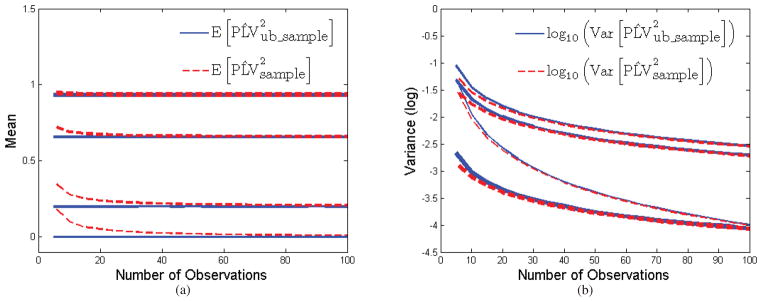
Bias and variance of ${\widehat{\text{PLV}}}_{\text{sample}}^2$ (red) and ${\widehat{\text{PLV}}}_{\text{ub}\_\text{sample}}^2$ (blue) as a function of N, the number of samples used to compute the estimators: (a) mean value vs N for four different true values of PLV; (b) variance vs. N for the same true values of PLV. Samples were drawn independently from the von Mises distribution for four different concentration parameter values.

2.2. Phase Locking Value and the von Mises Distribution

The von Mises distribution is the most widely used model for circular (or periodic) random variables, in part because it is the circular distribution with maximum entropy subject to constraints on its first trigonometric moments (Jammalamadaka and Sengupta, 2001). The probability density function (pdf) of the von Mises disribution is:

$$p(\phi |\mu ,\kappa )=\frac{1}{2\pi I_0(\kappa )}{e}^{\kappa cos(\phi -\mu )}$$ (13)

with concentration parameter κ ∈ [0, ∞) and mean $\mu \in \left[\begin{array}{cc}-\pi & \pi \end{array}\right]$; I₀(κ) is the modified Bessel function of zeroth order

$$I_0(\kappa )=\frac{1}{2\pi }{\int }_0^{2\pi }{e}^{\kappa cos(\theta )}d\theta .$$ (14)

The von Mises distribution is unimodal and symmetric about μ as illustrated in Fig. 2(a) for μ = 0. As the concentration parameter κ increases, the relative phase φ becomes increasingly concentrated about its mean. In the limit as κ goes to 0, it reduces to a uniform distribution corresponding to the case where the phases of the two signals are mutually independent.

Figure 2.

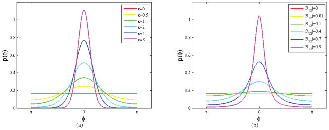
Probability density functions: (a) von Mises distribution with mean μ = 0 for a range of concentration values, κ; (b) relative phase distribution for bivariate circularly symmetric Gaussian models for different values of cross-correlation magnitude $\left|R_{12}\right|=\frac{{\kappa }_{12}}{\sqrt{{\kappa }_{11}{\kappa }_{22}}}$ with phase μ₁₂ = 0.

The PLV for the von Mises pdf can be found from the moment generating function:

$${\text{PLV}}_{\text{vonmises}}=\left|\text{E}\left[e^{j\mathrm{\Delta }\phi (t)}\right]\right|=\frac{I_1(\kappa )}{I_0(\kappa )}$$ (15)

as shown by Jammalamadaka and Sengupta (2001). The PLV is therefore a monotonic function of κ and independent of μ. In contrast, PLI can be found as:

$$\text{PLI}=\text{E}[\mathit{sign}(\mathrm{\Delta }\phi (t))]=\left|-{\int }_{-\pi }^{0}p(\phi |\mu ,\kappa )d\phi +{\int }_0^{\pi }p(\phi |\mu ,\kappa )d\phi \right|.$$ (16)

A closed form for this expression is intractable but it is clear that unlike PLV, PLI is a function of both κ and μ. We show this dependence in Fig. 3 for samples drawn from the von Mises distribution. This figure illustrates the monotonic relationship between PLV and κ and the more complex interaction between (κ, μ) and PLI.

Figure 3.

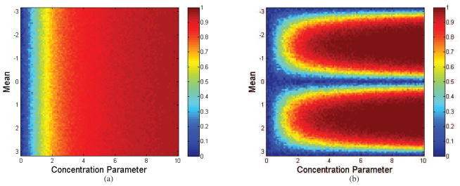
Plots of sample (a) PLV and (b) PLI as a function of concentration parameter κ and mean μ for samples drawn from the von Mises distribution. Note that while PLV is independent of μ, PLI depends on both κ and μ.

From equ. (15) we see that the PLV can be computed from an estimate of the concentration parameter κ. As shown in Jammalamadaka and Sengupta (2001), the maximum likelihood estimator of PLV for the von Mises distribution can be computed directly from a maximum likelihood estimator of κ and furthermore, the resulting estimator is identical to the sample PLV estimator in equ. (6):

$${\widehat{\text{PLV}}}_{\text{vonmises}}\triangleq \frac{I_1({\kappa }_{ML})}{I_0({\kappa }_{ML})}=\frac{1}{N}\left|\sum _{n=1}^N{e}^{j\mathrm{\Delta }{\phi }_n(t)}\right|={\widehat{\text{PLV}}}_{\text{sample}}.$$ (17)

2.3. Phase Locking Value and Circularly Symmetric Gaussian Processes

We now turn to an alternative statistical model for relative phase. Under the assumption that the time series whose phases are being compared are jointly Gaussian, then the distribution of their relative phase, and hence the PLV and PLI, must be governed by the properties and parameters of that Gaussian process. We now examine these relationships.

Let the sources s₁(t) and s₂(t) be jointly Gaussian zero mean processes. Then, the complex random vector $\mathbf{z}(t)={\left[\begin{array}{cc}{z}_1(t)& z_2(t)\end{array}\right]}^T$ where z_i(t) = s_i(t) + jHT (s_i(t)) = A_i(t)e^jφ_i(t) follows a circularly symmetric complex Gaussian distribution that satisfies the condition E[z(t)z(t)^T] = 0 and has the property that the real and imaginary components of z(t) are mutually independent (Gallager, 2008). The pdf of the circularly symmetric complex Gaussian distribution for a vector z(t) is

$$p(\mathbf{z}(t))=\frac{1}{{\pi }^2\left|{\mathbf{K}}_{\mathbf{z}}\right|}exp\left\{-\mathbf{z}{(t)}^H{\mathbf{K}}_{\mathbf{z}}^{-1}\mathbf{z}(t)\right\}$$ (18)

where, for the bivariate case ${\mathbf{K}}_{\mathbf{z}}\triangleq \left[\begin{array}{cc}{\kappa }_{11}& {\kappa }_{12}{e}^{j{\mu }_{12}}\\ {\kappa }_{12}{e}^{-j{\mu }_{12}}& {\kappa }_{22}\end{array}\right]=\text{E}\left[\mathbf{z}(t)\mathbf{z}{(t)}^H\right]$ is the covariance matrix of z(t), with 0 ≤ κ₁₂ < ∞ and −π ≤ μ₁₂ ≤ π. Inverting this matrix and normalizing gives the cross-correlation between z₁(t) and z₂(t) as $R_{12}\triangleq -\frac{{\kappa }_{12}}{\sqrt{{\kappa }_{11}{\kappa }_{22}}}{e}^{j{\mu }_{12}}$.

We rewrite the pdf in polar coordinates in order to investigate the relative phase distribution:

$$p(\mathbf{A}(t),\mathbf{\Phi }(t))=\frac{A_1(t)A_2(t)}{{\pi }^2\mid {\mathbf{K}}_{\mathbf{z}}\mid }exp\left\{-\left[\begin{array}{cc}{A}_1(t)e^{-j{\phi }_1(t)}& A_2(t)e^{-j{\phi }_2(t)}\end{array}\right]\left[\begin{array}{cc}{\kappa }_{11}& {\kappa }_{12}{e}^{j{\mu }_{12}}\\ {\kappa }_{12}{e}^{-j{\mu }_{12}}& {\kappa }_{22}\end{array}\right]\left[\begin{array}{c}{A}_1(t)e^{j{\phi }_1(t)}\\ A_2(t)e^{j{\phi }_2(t)}\end{array}\right]\right\}$$ (19)

$$=\frac{A_1(t)A_2(t)}{{\pi }^2\mid {\mathbf{K}}_{\mathbf{z}}\mid }exp\left\{-\sum _{i=1}^2{\kappa }_{ii}{A}_i{(t)}^2-2{\kappa }_{12}{A}_1(t)A_2(t)cos({\phi }_1(t)-{\phi }_2(t)-{\mu }_{12})\right\}$$ (20)

where $\mathbf{A}(t)\triangleq \left[\begin{array}{cc}{A}_1(t)& A_2(t)\end{array}\right]$ and $\mathbf{\Phi }(t)\triangleq \left[\begin{array}{cc}{\phi }_1(t)& {\phi }_2(t)\end{array}\right]$.

For the univariate case the circularly symmetric Gaussian pdf in polar form is separable. In other words, if we write z = Ae^iφ, then the density can be written p(z) = p(A, φ) = p(A)p(φ), where p(A) follows a Rayleigh distribution and p(φ) is uniform (Davenport and Root, 1958). However, this is not the case for the bivariate case, i.e. p(A(t), Φ(t)) ≠ p(A(t))p(Φ(t)), but rather the phase and amplitude are mutually coupled unless the cross-correlation is 0. We therefore now consider two different distributions for the relative phase Δφ(t) = (φ₁(t)−φ₂(t)): the distribution conditioned on the amplitudes, and the distribution in which we marginalize out the amplitudes.

From Bayes rule, the phase distribution conditioned on amplitude can be written as:

$$p(\mathbf{\Phi }(t)|\mathbf{A}(t))=\frac{p(\mathbf{A}(t),\mathbf{\Phi }(t))}{p(\mathbf{A}(t))}.$$ (21)

As shown in Appendix C, this results in the following conditional distribution for relative phase:

$$p(\mathrm{\Delta }\phi (t)|\mathbf{A}(t))=\frac{1}{2\pi I_0(-2{\kappa }_{12}{A}_1(t)A_2(t))}{e}^{-2{\kappa }_{12}{A}_1(t)A_2(t)cos(\mathrm{\Delta }\phi (t)-{\mu }_{12})}$$ (22)

Note that this has the form of a von Mises distribution, but with the mean and concentration parameters a function of not only the parameters of the Gaussian but also the amplitude of the observations. This result clearly shows that while we may be interested only in the relative phases of two signals, amplitude and phase are not independent, so that the amplitudes of the signals affect the relative phase distribution (and vice versa). Put another way, the amplitude and phase of jointly Gaussian signals do not contain independent information about those signals. Because of this amplitude dependence, to determine the distribution of the relative phase alone we need to marginalize with respect to amplitude, as also independently shown by Vo et al. (2011), to obtain the relative phase distribution:

$$p(\mathrm{\Delta }\phi (t))=\frac{1-{\left|R_{12}\right|}^2}{2\pi (1-{\gamma }^2)}\left(1-\frac{\gamma {\mathit{cos}}^{-1}(\gamma )}{\sqrt{(1-{\gamma }^2)}}\right)$$ (23)

where $R_{12}\triangleq -\frac{{\kappa }_{12}}{\sqrt{{\kappa }_{11}{\kappa }_{22}}}{e}^{j{\mu }_{12}}$ and γ ≜ |R₁₂|cos (Δφ(t) − μ₁₂). Note that in this case the relative phase is solely a function of the cross-correlation R₁₂ between z₁(t) and z₂(t), which also governs the correlation in amplitude between the two signals.

Fig. 2(b) shows plots of the relative phase distribution for the circularly symmetric complex Gaussian model for different values of R₁₂ with μ₁₂ = 0. Varying μ₁₂ from zero will circularly shift the distribution so that its maximum is at μ₁₂. In comparison to the von Mises distribution, |R₁₂| plays the role of the concentration parameter, and μ₁₂ the mean. However, there are differences in the shapes of these two distributions, with the Gaussian case showing slightly longer tailed behavior.

Using the moment generating function of the relative phase PDF (equ. 23), as we show in Appendix D, we find the phase locking value for the circularly symmetric Gaussian model is

$$\begin{array}{l}{\text{PLV}}_{\text{circgauss}}\triangleq \left|\text{E}\left[e^{j\mathrm{\Delta }\phi (t)}\right]\right|\\ =\left|\frac{\pi }{\sqrt{2}}\left(1-\frac{{\kappa }_{11}{\kappa }_{22}}{{\kappa }_{12}^2}\right)\left[{w^{3/2}}_2{F}_1\left(\frac{3}{4},\frac{5}{4},1,w^2\right)+\frac{3}{4}{w^{5/2}}_2{F}_1\left(\frac{5}{4},\frac{7}{4},2,w^2\right)\right]\right|\end{array}$$ (24)

where $w\triangleq \frac{{\kappa }_{12}^2}{2{\kappa }_{11}{\kappa }_{22}-{\kappa }_{12}^2}$ and ₂F₁(.) represents the hypergeometric function. Note that PLV is a function of the magnitude of the cross-correlation $\left|R_{12}\right|={\kappa }_{12}/\sqrt{{\kappa }_{11}{\kappa }_{22}}$. Fig. 4 shows this one-to-one relationship. The significance of this result is as follows. The parameter κ₁₂/κ₁₁κ₂₂ represents the magnitude of the cross-correlation between the two complex Gaussian processes z₁(t) and z₂(t). If these are narrow-band signals, the cross-correlation at a single frequency is equivalent to coherence between the two processes at that frequency. Consequently, PLV and coherence are equivalent measures. Of course, this holds only for the Gaussian case, and we will return to the question of whether electrophysiological signals can be adequately modeled as jointly Gaussian in the following section.

Figure 4.

Plot of the monotonic relationship between PLV and the magnitude of cross-correlation, $\left|R_{12}\right|=\frac{{\kappa }_{12}}{\sqrt{{\kappa }_{11}{\kappa }_{22}}}$, for the bivariate circularly symmetric Gaussian model.

As with the von Mises case, we do not have a closed form for PLI using the integral in equ. (16) after substituting in the relative phase distribution in equ. (23) for the Gaussian case. However, we can determine the relationship between PLI and the Gaussian parameters (|R₁₂|, μ₁₂) by Monte Carlo sampling. We generated samples from the relative phase distribution in equ. (23) for a range of values of |R₁₂| and μ₁₂. Fig. 5 shows sample estimates of PLV and PLI as a function of these two parameters. Again, similarly to the von Mises case, while PLV depends only on the |R₁₂| value, PLI is a function of both |R₁₂| and μ₁₂.

Figure 5.

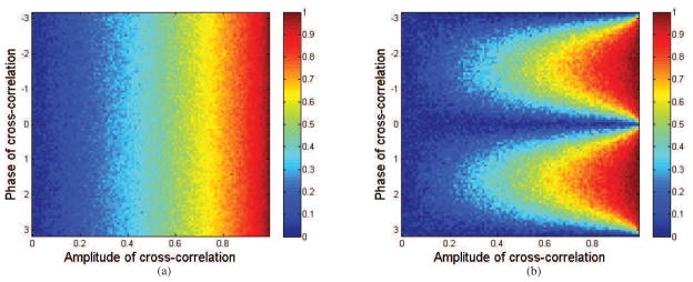
Plots of sample (a) PLV and (b) PLI as a function of cross-correlation magnitude $\left|R_{12}\right|=\frac{{\kappa }_{12}}{\sqrt{{\kappa }_{11}{\kappa }_{22}}}$ and phase μ₁₂ for the bivariate circularly symmetric Gaussian distribution. Similarly to the von Mises distribution, PLV is independent of phase while PLI depends on both cross-correlation magnitude and phase. Samples were drawn from relative phase distribution in equ. (23).

The relationship in equ. (24) between cross-correlation and PLV also gives us an alternative estimator for the latter. Rather than directly computing sample PLV, we can instead compute the sample estimator of |R₁₂| and then substitute this into equ. (24). We refer to this estimator as ${\widehat{\text{PLV}}}_{\text{circgauss}}$. In the following section we compare this with the sample PLV estimate in both simulated and experimental LFP data.

3. Results

3.1. Simulations Based on the Gaussian distribution

In the previous section we described three different estimators for the PLV: ${\widehat{\text{PLV}}}_{\text{sample}}$ (equ. 6), $\sqrt{{\widehat{\text{PLV}}}_{\text{ub}\_\text{sample}}^2}$ (equ. 11), and ${\widehat{\text{PLV}}}_{\text{circgauss}}$ (the PLV computed from the sample cross-correlation, Equ. 24). Their relative performance in terms of bias and variance will depend on the true distribution of the data. Before considering the case of experimental electrophysiological data, we will first explore their behavior for simulated bivariate Gaussian processes.

We generated independent samples from two different bivariate Gaussian processes with normalized cross-correlation values of |R₁₂| = 0.25 and |R₁₂| = 0.91, with analytic PLV values of 0.20 and 0.83, respectively. This was achieved by multiplying pairs of independent zero mean uncorrelated Gaussian random variables by the inverse square root of the 2 × 2 covariance matrix $\left[\begin{array}{cc}1& R_{12}\\ R_{12}& 1\end{array}\right]$. We then generated the complex signal by applying the Hilbert transform to the bivariate sequences using Matlab’s discrete Fourier transform based “Hilbert” function. For both values of correlation we computed ${\widehat{\text{PLV}}}_{\text{sample}},\sqrt{{\widehat{\text{PLV}}}_{\text{ub}\_\text{sample}}^2}$, and ${\widehat{\text{PLV}}}_{\text{circgauss}}$ as a function of sample size N. A total of 1,000 Monte Carlo trials were performed for each value of cross-correlation and N, and sample means and variances computed for each measure of PLV. Results are plotted in Fig. 6.

Figure 6.

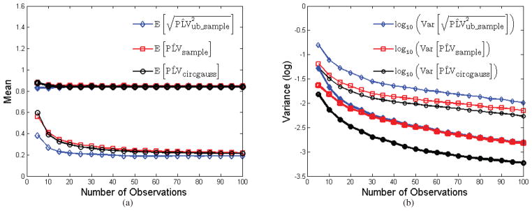
Plot of bias and variance for the sample PLV, root of unbiased sample PLV, and PLV computed from sample cross-correlation. (a) plot of the mean over 1,000 Monte Carlo trials as a function of number of samples used to estimate the parameter for two different values of cross-correlation; (b) corresponding plot of variance for each of the three estimators for the two different cross-correlation values. Samples were drawn independently from bivariate Gaussian processes.

All three measures exhibit bias for small N. Note that while ${\widehat{\text{PLV}}}_{\text{ub}\_\text{sample}}^2$ is an unbiased estimator of PLV², its square root is not an unbiased estimator of PLV although it does exhibit the lowest bias among the three estimators. As expected, ${\widehat{\text{PLV}}}_{\text{ub}\_\text{sample}}$ also has the largest variance. It is also clear from Fig. 6 that the variance when estimating PLV from the cross-correlation is significantly smaller than that of ${\widehat{\text{PLV}}}_{\text{sample}}$. Consequently, for data that are approximately Gaussian, using cross-correlation to compute phase locking gives a more reliable (lower variance) interaction measure than does sample PLV. In comparison, in the case of the von Mises distribution, we saw that the sample PLV is a maximum likelihood estimator which is asymptotically efficient and in practice tends to exhibit close to minimum variance behavior even for small sample sizes.

3.2. Roessler Oscillator Simulations

Roessler oscillators are commonly used models of weakly coupled stochastic oscillators. We generated two Roessler oscillators ξ₁ and ξ₂ using the equations described in Schelter et al. (2006):

$$\begin{array}{l}{\xi }_j=\left(\begin{array}{c}{\stackrel{.}{X}}_j\\ {\stackrel{.}{Y}}_j\\ {\stackrel{.}{Z}}_j\end{array}\right)\\ =\left(\begin{array}{c}-{\omega }_j{Y}_j-Z_j+\left[{\mathrm{\sum }}_{i\ne j}{\epsilon }_{i,j}(X_i-X_j)\right]+\sigma {\eta }_j\\ {\omega }_j{X}_j+{aY}_j\\ b+(X_j-c)Z_j\end{array}\right)\end{array}$$ (25)

where i, j ∈ {1, 2}. The parameters were a = 0.5, b = 0.2, c = 10, ω₁ = 1.03, ω₂ = 1.01 and η_j is standard Gaussian noise. A range of values of σ were used as shown in Fig. 7. Parameter ε_{i, j} controls the amount of coupling from the i^th to the j^th oscillator and is set such that ε₁₂ = ε₂₁ = ε implying a bidirectional coupling. In this study we consider two cases: coupling (ε > 0) and no coupling (ε = 0). For each of 1, 000 trials we generated time series up to length 9, 000 samples with a sample interval Δt = 0.02.

Figure 7.

Roessler oscillator simulations (a) Comparison of ROC curves of ${\widehat{\text{PLV}}}_{\text{circgauss}}$ (blue) and ${\widehat{\text{PLV}}}_{\text{sample}}$ (red) when ε = 0.15 for coupled oscillators, standard deviation σ = 1.5 and number of samples L = 5000. (b) Area under ROC curve as a function of coupling parameter ε when σ = 1.5 and L = 5000. (c) Area under ROC curve as a function of number of samples L when σ = 1.5 and ε = 0.15. (d) Area under ROC curve as a function of the standard deviation of the noise σ when L = 5000 and ε = 0.15.

We used the simulated time series X₁ and X₂ to investigate the behavior of ${\widehat{\text{PLV}}}_{\text{sample}}$ and ${\widehat{\text{PLV}}}_{\text{circgauss}}$ for the cases with and without coupling. We generated receiver operating characteristic (ROC) curves (Swets, 1996) showing the fraction of true positive values (PLV > τ when ε > 0) versus false positives (PLV > τ when ε = 0) as a function of the threshold τ. Comparing the ROC curves for the two different PLV estimators we can determine which has the better sensitivity vs. specificity performance, as indicated by the area under the curve, AUC (an AUC = 1 represents error free detection).

A sample ROC curve is shown in Fig. 7(a) for the two estimators, indicating superior detection performance for ${\widehat{\text{PLV}}}_{\text{circgauss}}$ compared to ${\widehat{\text{PLV}}}_{\text{sample}}$. Figs 7b–d show the AUCs for the ROC curves over range of (b) coupling parameters, (c) number of samples, and (d) variances. Results consistently show superior performance for ${\widehat{\text{PLV}}}_{\text{circgauss}}$, particularly for small values of the coupling parameter and for a relatively small number of samples. As these parameters increase, results for both estimators are similar. Since the ${\widehat{\text{PLV}}}_{\text{circgauss}}$ is a deterministic monotonic function of the sample cross-correlation, it follows that identical ROC curves would be obtained by replacing ${\widehat{\text{PLV}}}_{\text{circgauss}}$ with the sample cross-correlation. These results indicate that even in the cases where the data are not Gaussian, PLV calculation based on the Gaussian model (or equivalently, the sample cross-correlation) can give superior detection of coupling than can be achieved using the sample PLV. This seems to indicate that care should be taken in interpreting PLVs, since they do not necessarily provide different or more reliable insight into data than does the sample correlation. This is the case even in this case where the data are not obviously Gaussian. We now turn to the case for experimental data.

3.3. Analysis of LFP data

Phase locking values have been used to analyze invasive (cortical and depth electrode) and noninvasive (EEG, MEG) recordings. In our work we are interested in modeling signals ranging in scale from local field potentials from microelectrodes through invasive recordings with larger electrodes as well as EEG and MEG. Of these, microelectrode LFPs have the most localized sensitivity. The other recordings can be viewed as equivalent to linear mappings of LFPs at the cortical level (or equivalently, the combination of dendritic and volume current sources that give rise to them) by integration with respect to the field sensitivities of the electrodes or magnetometers. These macro recordings should therefore be more Gaussian than the microrecordings through a law of large numbers argument. Conversely, multiunit and single unit recordings reflect the spiking activity associated with action potentials, and we would expect these to be highly non-Gaussian. Here we investigate the degree to which LFP recordings can be assumed to be Gaussian from the perspective of their relative phase distributions. In other words, we explore whether PLVs computed from cross-correlations produce equivalent results to those computed directly using the sample PLV.

For this study we used the LFP data described by Bressler et al. (1993), which has been widely studied over the past two decades (Bressler, 1995; Bressler et al., 1999; Ding et al., 2000; Brovelli et al., 2004). Recordings were made using 51 μm diameter bipolar electrodes separated by 2.5 mm in macaque monkeys. Measurements from a total of 15 electrode pairs in the right hemisphere, with approximate locations shown in Fig. 8, were analyzed. In the experiment the monkey was trained to depress a lever and wait for a visual cue to either go (release) or no-go (not release). The go and no-go cues were a diamond and line pattern as shown in Fig. 9, with the choice of diamond or line as the go cue changing between experiments. The cue was given 115ms after the lever was depressed, and a reward given if the monkey responded correctly to the go cue within 500ms. In the results presented below, we examine phase-locking at two time intervals: early response (120 ± 25 msec after cue) and late response (260 ± 25 msec after cue). Data were originally sampled at 200Hz and bad trials discarded. The remaining 10, 178 trials contained 5225 go trials (go cue is line for 2322 trials and diamond for 2903 trials) and 4953 no-go trials (no-go cue is diamond for 2407 trials and line for 2546 trials). For this study, the data for each channel and trial was first band-pass filtered to a frequency band 13–30 Hz by using two-way elliptic IIR filtering of order 14. Hilbert transforms were then applied to each of these time series using Matlab’s “Hilbert” transform function. Because of the use of bipolar electrodes, the data should not be sensitive to volume conduction effects and therefore we restrict attention here to PLV and do not compute PLI.

Figure 8.

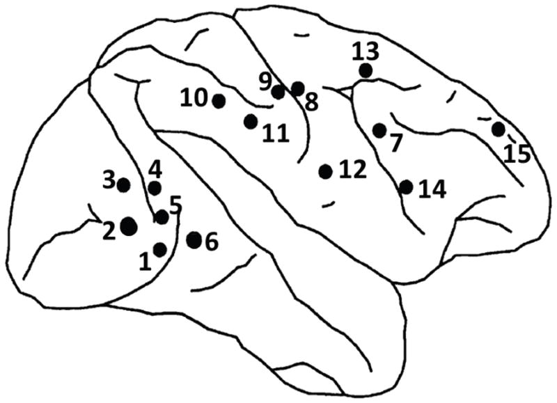
Locations of 15 electrode pairs in the right hemisphere (reproduced from Liang et al. (2001))

Figure 9.

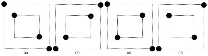
Four visual cues represented to the monkey in the experiment (a) right slanted line (b) left slanted line (c) right slanted diamond (d) left slanted diamond.

We first consider the relative phase distribution between pairs of electrodes. In Fig. 10, we show goodness of fit between the empirical relative phase distribution extracted from LFP data and the theoretical distributions based on von Mises and circularly symmetric Gaussian models. To compute the theoretical distributions we assumed zero mean and estimated the concentration (for von Mises) and cross-correlation (for Gaussian) parameters from the sample data. The electrodes and the tasks are selected based on the results represented in Table 2 which will be discussed later. The common feature of all selected electrodes is that they represent significant interaction when using sample PLV and circularly symmetric Gaussian PLV. We used a chi-square goodness of fit test for the two distributions (Lancaster and Seneta, 2005). We list the p-values for the selected pairs in Table 1. We were unable to reject the null hypothesis at α = 0.05 for either distribution for any pairs shown, with the exception that the von Mises was rejected between electrodes 3 and 5 at 120 msec as shown in Fig. 10(c) and listed in Table 1. We also plot ${\widehat{\text{PLV}}}_{\text{sample}}$ versus ${\widehat{\text{PLV}}}_{\text{circgauss}}$ using all pairwise combinations in Fig. 11. We can conclude from these results that either distribution is probably adequate to represent the true phase relationships in this LFP data.

Figure 10.

Goodness of fit between empirical distribution of relative phase extracted from LFP data and parametric von Mises and circularly symmetric Gaussian distributions. The concentration parameter (von Mises) and cross-correlation parameter (Gaussian) were directly estimated from the sample data. (a–c) pairs at 120 msec (d–h) pairs at 260 msec

Table 2.

Comparison of the number of experiments showing significant interactions between electrode pairs for each of four conditions (Diamond, line, go, no-go) computed using sample PLV and Gaussian PLV for early and late response periods. Significance was assessed using FDR = 0.01 based on permutations of trial indices. Only pairs for which a minimum of 5 experiments show significant interactions in either cue or task based comparison are shown.

PLV type	Early Response:					Late Response:
sample	Pair	Diamond	Line	GO	NO-GO	Pair	Diamond	Line	GO	NO-GO
	2–3	8	0	5	3	1–7	4	3	7	0
	2–5	14	0	9	5	1–8	6	4	10	0
	3–5	8	0	4	4	4–7	4	1	5	0
						4–8	6	5	11	0
						7–8	4	5	9	0
Gaussian	Pair	Diamond	Line	GO	NO-GO	Pair	GO	NO-GO	Diamond	Line
	2–3	9	0	5	4	1–7	3	4	7	0
	2–5	17	0	10	7	1–8	5	6	11	0
	3–5	10	0	5	5	4–7	3	4	7	0
						4–8	6	6	12	0
						7–8	5	2	10	0

Table 1.

The p-values of Chi-square statistic for goodness of fit of the von Mises and circularly symmetric Gaussian phase models. In only on case are we able to reject the null hypothesis: electrode pair 3 and 5 for the von Mises model.

Electrode Pairs	von Mises	Gaussian
2 and 3 at 120 msec	0.97	0.99
2 and 5 at 120 msec	0.55	0.53
3 and 5 at 120 msec	0	0.51
1 and 7 at 260 msec	0.48	0.54
1 and 8 at 260 msec	0.47	0.61
4 and 7 at 260 msec	0.50	0.85
4 and 8 at 260 msec	0.43	0.54
7 and 8 at 260 msec	0.09	0.46

Figure 11.

Scatter plot of ${\widehat{\text{PLV}}}_{\text{vonimises}}$ versus ${\widehat{\text{PLV}}}_{\text{circgauss}}$ computed from macaque LFP data.

We computed ${\widehat{\text{PLV}}}_{\text{sample}}$ and ${\widehat{\text{PLV}}}_{\text{circgauss}}$ for each electrode pair for each of the 18 experiments for the early and late intervals with trials sorted in two ways: (a) by visual cue (diamond vs. line) and (b) task (go vs no-go). Since the visual cues were switched in different experiments, the two different groupings allow us to differentiate interactions associated with cue vs. those associated with task.

To assess significance of interactions we applied permutation testing by trial-shuffiing within electrode pairs to obtain a null distribution (no interaction). Using these distributions, computed separately for each pair and each condition, we then converted the PLV values to p-values. We account for multiple hypotheses testing by thresholding with a false discovery rate (FDR) of 0.01. For each pair we then computed the number of experiments (out of 18) in which PLV values indicated a significant interaction. Results are reported in Table 2 and illustrated in Fig. 12. Only pairs showing a minimum of 5 out of 18 experiments in either cue or task based comparison with significant PLVs are included in Table 2 whereas no threshold was applied for representation of results in Fig. 12.

Figure 12.

Phase synchronization networks constructed from the results in Table 2. Green: significant PLVs occur when diamond is presented. Magenta: significant PLVs occur when line is presented. Blue: significant PLVs occur during go condition. Red: significant PLVs occur during no-go condition. The thickness of the edges represents the number of experiments sessions in which significant synchronization occurs.

In Table 2 we report the electrode pairs with significant PLVs for diamond vs. line and for go vs. no-go for both the early and late period. These results are included for two different PLV estimators: ${\widehat{\text{PLV}}}_{\text{sample}}$ , which is the ML estimator for the von Mises distribution, and ${\widehat{\text{PLV}}}_{\text{circgauss}}$. Consider first the results for ${\widehat{\text{PLV}}}_{\text{sample}}$. For the early response we consistently see significant PLVs between electrode pairs 2–3, 2–5 and 3–5 for the diamond stimulus while there are none for the line. For this same early period, when sorting trials by go vs. no-go (both of which contain diamond and line stimuli) we see no indication that the go condition produces consistently more significant PLVs than the no-go condition. Note that electrode pairs 2–3, 2–5 and 3–5 are in striate/pre-striate cortex.

If we now look at results for the late response we see that the above observation is now largely reversed. In this case it is the go condition that leads to significant interactions between striate/prestriate and motor/pre-motor cortices (pairs 1–7, 1–8, 4–7, 4–8, 7–8) while the no-go condition shows no significant interactions for any of these pairs. If the same data are sorted according to diamond vs. line we see no clear preference for significant interactions. These results might be expected since the early response (120 ± 25 msec after cue) should reflect visual processing while the later response (260 ± 25 msec after cue) should also include visual/motor interactions. We now turn to the comparison in Table 2 between the two PLV estimators. While the number of experiments showing significant interactions is not identical between the top and bottom halves of the table, the pairs of electrodes showing significant interactions are exactly the same for the two estimators, with very close agreement between the number of experiments with significant interactions for diamond vs. line in the early response and go vs. no-go for the late response. The Gaussian model consistently produces equal or slightly larger number of significant interactions in each column in the table, possibly reflecting superior detection power resulting from the lower variance of the estimator shown in Fig. 6.

4. Discussion and Conclusion

The primary purpose of this paper was to explore the properties of the phase locking value as it is frequently applied to electrophysiological data, i.e. as a measure of variability of the relative phase between two signals computed by averaging over multiple trials and relatively short time windows (Mormann et al., 2000; Lachaux et al., 2000; Varela et al., 2001; Bhattacharya et al., 2001; Doesburg et al., 2008; Ossadtchi et al., 2010).

The sample PLV is a biased measure, as previously shown by Vinck et al. (2010). While the degree of bias depends on distribution, the bias in the squared sample PLV was shown to be a simple function of sample size N, equ. (10). Rearranging this result produces an unbiased estimator, equ. (11). It is interesting to note that this result is identical to Vinck’s PPC (Pairwise Phase Consistency) measure. In practice bias is relatively small for N > 50 so that the sample PLV should be adequate unless sample size is small.

The sample PLV is a maximum likelihood estimator when the data follow a von Mises distribution implying efficiency of the estimator. We also saw that PLV is a monotonic function of the concentration parameter and independent of the mean. Similarly we also saw that for jointly Gaussian data, the PLV is a monotonic function of cross-correlation and also independent of mean. This latter result was based on marginalizing the joint density for the complex representation of the two signals with respect to the signal amplitudes leaving a distribution as a function of relative phase. In contrast to the von Mises case, the sample PLV is not a maximum likelihood estimator, and in fact we saw from Fig. 6 that computing PLV directly from the sample cross-correlation leads to a lower variance estimate than the sample PLV.

It is not surprising that PLV depends only on cross correlation for Gaussian signals, since jointly Gaussian processes are completely characterized by their mean and covariance. Nevertheless, the consequence of this observation is perhaps less obvious: that if data are reasonably well modeled as jointly Gaussian, then the PLV provides no information that is not already contained in the cross correlation. We saw that this appears to be the case for the macaque LFP data analyzed above as well as the simulation based on the Roessler oscillator. Comparing sample PLV results with a PLV computed directly from the sample cross-correlation we see very little difference between results in terms of the pairs of electrodes exhibiting significant interaction when using the two different measures. The distribution plots in Fig. 10, and associated hypothesis tests in Table 1, indicate that both the von Mises and circularly symmetric Gaussian distributions are adequate for this data. This supports the earlier statement that PLV does not add information not contained in the cross correlation.

It appears reasonable to expect that similar results to these LFP studies would be obtained when analyzing MEG and EEG data, since they share with the LFP a dependence primarily on dendritic currents and the associated volume or conduction currents. Differences between these data depend on the lead field sensitivities of the transducers, with MEG and EEG being sensitive to far larger regions of cortex than the microelectrodes used to acquire the data in the study. Through the law of large numbers, we would expect as we integrate over larger regions of cortical activation, that data would tend to become more rather than less Gaussian.

It is important to note that the above observations are applicable only to data that can be considered approximately stationary over the interval over which the PLV is calculated. This is frequently the case in published studies, where either PLV is calculated over a short time window, or using a single time sample and averaging over trials (Lachaux et al., 2003, 2000; Hurtado et al., 2004; Rudrauf et al., 2006). If PLV is computed over longer time periods for which the behavior cannot be considered to be stationary, then the equivalence of PLV and cross-correlation would not necessary be retained. We also emphasize that the above arguments apply only to LFPs, EEG and MEG. Multiunit recordings are clearly non-Gaussian and we would not expect to see equivalence in this case.

In several instances false phase locking can arise as a result of linear mixing or cross-talk between time series: (a) use of common reference in microelectrode or EEG recordings, (b) EEG or MEG recordings with overlapping sensitivities in the lead field, and (c) cortical current density maps computed from EEG or MEG data in which the low resolution causes interference between sources. Since the PLV is independent of the mean phase difference, this measure cannot differentiate between a zero-mean phase difference, which can be explained by linear mixing, and a non-zero phase lag, which cannot be caused by linear mixing. The Phase Lag Index (PLI) was designed to be robust to this problem. In Figures 3 and 5 we show the dependence of PLI on the parameters of both the von Mises and Gaussian distributions. Unlike PLV, PLI is a function of the mean as well as the variance of relative phase. While this does produce the desired robustness to linear mixing, it is also a function of both mean and variance so that it is not possible to assess the strength of the interaction without also knowing the phase. One solution to this problem might be to compute both the mean and PLV of the relative phase, and use the mean to test for linear mixing and the PLV to assess the strength of the detected interaction. A similar problem is encountered when using coherence as an interaction measure: a real value of coherence can arise simply due to linear mixing. An effective solution to this problem is to use only the imaginary part of coherence (Nolte et al., 2004), which cannot be nonzero without true interaction. We note that even in the Gaussian case, where PLV and cross-correlation are equivalent, the PLI and imaginary coherence are not: while both depend on the complex value rather than the magnitude of the cross-correlation, they are different functions of this parameter.

Interactions between neuronal populations are not pairwise, but typically involve multiple areas or electrodes. When computing pairwise correlations, interactions between pairs can be produced even if the pair does not have a direct interaction but instead both of the areas are interacting with a third. For this reason, multinode network models are sometimes inferred using a multivariate model in which partial correlations are computed to differentiate direct from indirect interactions between electrode pairs. These networks can be represented using multivariate Gaussian models where the partial correlations are given by the non-zero entries of the inverse of the correlation matrix (Whittaker, 2009; Mima et al., 2000). Recently Canolty et al. (2012) have developed a multivariate extension of the von Mises distribution that similarly is able to differentiate between direct and indirect interactions, but with respect to phase coupling rather than correlation. It would be interesting to explore differences between partial correlation and partial phase in LFP, EEG and MEG networks, since the relationships explored here between PLV and cross-correlation could in principle be extended to multivariate Gaussian models.

Highlights.

• We explore the properties of the Phase Locking Value as a measure of phase coupling

• We relate the PLV to the parameters of the von Mises distribution

• We relate the PLV to parameters of complex circularly symmetric Gaussian processes

• We compare PLV with cross-correlation in bivariate LFP data

• We show that for the LFP data used here, these measures are equivalent

Appendices

A. Bias of Squared PLV

Here we derive an expression for the bias of ${\widehat{\text{PLV}}}_{\text{sample}}^{\text{2}}$.

$$\text{E}\left[{\widehat{\text{PLV}}}_{\text{sample}}^{\text{2}}\right]=\text{E}\left[{\left|\frac{1}{N}\sum _{n=1}^N{e}^{j\mathrm{\Delta }{\phi }_n}\right|}^2\right]=\frac{1}{N^2}\text{E}\left[\sum _{n=1}^N{e}^{j\mathrm{\Delta }{\phi }_n}\sum _{m=1}^N{e}^{-j\mathrm{\Delta }{\phi }_m}\right]$$ (26)

$$=\frac{1}{N^2}\left(N+\sum _{n=1}^N\sum _{m\ne n}^N\text{E}\left[e^{j(\mathrm{\Delta }{\phi }_n-\mathrm{\Delta }{\phi }_m}\right]\right)$$ (27)

Assuming Δφ_n and Δφ_m are independent for n ≠ m

$$=\frac{1}{N^2}\left(N+\sum _{n=1}^N\sum _{m\ne n}^N\text{E}\left[e^{j\mathrm{\Delta }{\phi }_n}\right]\text{E}\left[e^{-j\mathrm{\Delta }{\phi }_m}\right]\right)$$ (28)

$$=\frac{1}{N^2}\left(N+(N^2-N){\left|\text{E}\left[e^{j\mathrm{\Delta }\phi }\right]\right|}^2\right)=\frac{1}{N}+\left(1-\frac{1}{N}\right){\text{PLV}}^2$$ (29)

B. Unbiased square PLV and PPC

Rearranging equ. (29), gives the following unbiased estimate of PLV²:

$${\widehat{\text{PLV}}}_{\text{ub}\_\text{sample}}^2=\frac{1}{N-1}\left({\widehat{\text{PLV}}}_{\text{sample}}^2\times N-1\right)$$ (30)

Further manipulation of this expression shows it is equivalent to the pairwise phase consistency (PPC) measure of Vinck.

$$=\frac{1}{N-1}\left[\frac{1}{N}{\left|\sum _{n=1}^N{e}^{j\mathrm{\Delta }{\phi }_n}\right|}^2-1\right]$$ (31)

$$=\frac{1}{N(N-1)}\left[N+\sum _{n=1}^N\sum _{m\ne n}^N{e}^{j(\mathrm{\Delta }{\phi }_m-\mathrm{\Delta }{\phi }_n)}\right]-\frac{1}{N-1}$$ (32)

$$=\frac{1}{N(N-1)}\underset{{\sum }_{n=1}^{N-1}{\sum }_{m>n}^N{e}^{j(\mathrm{\Delta }{\phi }_m-\mathrm{\Delta }{\phi }_n)}+{\sum }_{n=1}^N{\sum }_{m<n}^{N-1}{e}^{j(\mathrm{\Delta }{\phi }_m-\mathrm{\Delta }{\phi }_n)}}{\underbrace{\sum _{n=1}^N\sum _{m\ne n}^N{e}^{j(\mathrm{\Delta }{\phi }_m-\mathrm{\Delta }{\phi }_n)}}}$$ (33)

$$=\frac{2}{N(N-1)}\sum _{n=1}^{N-1}\sum _{m=n+1}^N\mathit{cos}(\mathrm{\Delta }{\phi }_m-\mathrm{\Delta }{\phi }_n)$$ (34)

which is the PPC measure in equ. 12 in Vinck et al. (2010).

C. Conditional Distribution of Relative Phase for the Bivariate Circularly Symmetric Complex Gaussian

First, we need to find an expression for the marginal distribution of amplitudes A(t)

$$p(\mathbf{A}(t))={\int }_0^{2\pi }{\int }_0^{2\pi }p(\mathbf{A}(t),\mathbf{\Phi }(t))d{\phi }_1(t)d{\phi }_2(t)$$ (35)

from equ. (20)

$$=\frac{A_1(t)A_2(t)}{{\pi }^2\mid {\mathbf{K}}_{\mathbf{z}}\mid }exp\left(-\sum _{i=1}^2{\kappa }_{ii}{A}_i^2(t)\right)\underset{4{\pi }^2{I}_0(-2{\kappa }_{12}{A}_1(t)A_2(t))}{\underbrace{{\int }_0^{2\pi }{\int }_0^{2\pi }exp(-2{\kappa }_{12}{A}_1(t)A_2(t)cos({\phi }_1(t)-{\phi }_2(t)-{\mu }_{12}))d{\phi }_1(t)d{\phi }_2(t)}}$$ (36)

$$=\frac{4A_1(t)A_2(t)I_0(-2{\kappa }_{12}{A}_1(t)A_2(t))}{\mid {\mathbf{K}}_{\mathbf{z}}\mid }exp\left(-\sum _{i=1}^2{\kappa }_{ii}{A}_i^2(t)\right).$$ (37)

Substituting this result into equ. (21), we get

$$p(\mathrm{\Phi }(t)\mid \mathbf{A}(t))=\frac{\frac{A_1(t)A_2(t)}{{\pi }^2\left|{\mathbf{K}}_{\mathbf{z}}\right|}exp\left\{-{\sum }_{i=1}^2{\kappa }_{ii}{A}_i^2(t)-2{\kappa }_{12}{A}_1(t)A_2(t)cos({\phi }_1(t)-{\phi }_2(t)-{\mu }_{12})\right\}}{\frac{4A_1(t)A_2(t)I_0(-2{\kappa }_{12}{A}_1(t)A_2(t))}{\left|{\mathbf{K}}_{\mathbf{z}}\right|}exp\left(-{\sum }_{i=1}^2{\kappa }_{ii}{A}_1^2(t)\right)}$$ (38)

$$=\frac{1}{4{\pi }^2{I}_0(-2{\kappa }_{12}{A}_1(t)A_2(t))}{e}^{-2{\kappa }_{12}{A}_1(t)A_2(t)cos({\phi }_1(t)-{\phi }_2(t)-{\mu }_{12})}$$ (39)

D. The PLV for the Bivariate Circularly Symmetric Complex Gaussian

$$\text{E}[e^{j\mathrm{\Delta }\phi (t)}]=\text{E}\left[\text{E}\left[e^{j\mathrm{\Delta }\phi (t)}\mid A_1(t),A_2(t)|\right]\right]$$ (40)

using the first moment generating function of von Mises distribution:

$$=\text{E}\left[\frac{I_1(-2{\kappa }_{12}{A}_1(t)A_2(t))}{I_0(2{\kappa }_{12}{A}_1(t)A_2(t))}\right]$$ (41)

$$={\int }_0^{\infty }{\int }_0^{\infty }\frac{I_1(-2{\kappa }_{12}{A}_1(t)A_2(t))}{I_0(2{\kappa }_{12}{A}_1(t)A_2(t))}p(A_1(t),A_2(t)){dA}_1(t){dA}_2(t)$$ (42)

using the result in equ. 37:

$$=\frac{4}{\mathit{det}({\mathbf{K}}_{\mathbf{z}})}{\int }_0^{\infty }{\int }_0^{\infty }\underset{\frac{1}{\pi }{\int }_{-\pi /2}^{\pi /2}{e}^{-2{\kappa }_{12}{A}_1(t)A_2(t)sin(\theta )}sin(\theta )d\theta }{\underbrace{I_1(-2{\kappa }_{12}{A}_1(t)A_2(t))}}{A}_1(t)A_2(t)e^{-{\kappa }_{11}{A}_1^2(t)-{\kappa }_{22}{A}_2^2(t)}{dA}_1(t){dA}_2(t)$$ (43)

$$=\frac{4}{\mathit{det}({\mathbf{K}}_{\mathbf{z}})\pi }{\int }_0^{\infty }{\int }_0^{\infty }{\int }_{-\pi /2}^{\pi /2}{A}_1(t)A_2(t)sin(\theta )e^{-{\kappa }_{11}{A}_1^2(t)+2{\kappa }_{12}{A}_1(t)A_2(t)sin\theta -{\kappa }_{22}{A}_2^2(t)}{dA}_1(t){dA}_2(t)d\theta$$ (44)

$$\frac{4}{\mathit{det}({\mathbf{K}}_{\mathbf{z}})\pi }{\int }_{-\pi /2}^{\pi /2}sin(\theta ){\int }_0^{\infty }{A}_2(t)e^{-{\kappa }_{22}{A}_2^2(t)}\underset{\triangleq B(\theta ,A_2(t),{\kappa }_{11},{\kappa }_{12})}{\underbrace{{\int }_0^{\infty }{A}_1(t)e^{-{\kappa }_{11}{A}_1^2(t)+2{\kappa }_{12}{A}_1(t)A_2(t)sin(\theta )}{dA}_1(t)}}{dA}_2(t)d\theta$$ (45)

$$B(\theta ,A_2(t),{\kappa }_{11},{\kappa }_{12})={\int }_0^{\infty }{A}_1(t)e^{-{\kappa }_{11}\left(A_1^2(t)-\frac{2{\kappa }_{12}{A}_2(t)sin(\theta )}{{\kappa }_{11}}{A}_1(t)\right)}{dA}_1(t)$$ (46)

$$e^{\frac{{\kappa }_{12}^2{A}_2^2(t){sin}^2(\theta )}{{\kappa }_{11}}}{\int }_0^{\infty }{A}_1(t)e^{-{\kappa }_{11}\left(A_1^2(t)-\frac{2{\kappa }_{12}{A}_2(t)sin(\theta )}{{\kappa }_{11}}{A}_1(t)+\frac{{\kappa }_{12}^2{A}_2^2(t){sin}^2(\theta )}{{\kappa }_{11}^2}\right)}{dA}_1(t)$$ (47)

$$=e^{\frac{{\kappa }_{12}^2{A}_2^2(t){sin}^2(\theta )}{{\kappa }_{11}}}{\int }_0^{\infty }{A}_1(t)e^{-{\kappa }_{11}{\left(A_1(t)-\frac{{\kappa }_{12}{A}_{2}sin(\theta )}{{\kappa }_{11}}\right)}^2}{dA}_1(t)$$ (48)

$$=e^{\frac{{\kappa }_{12}^2{A}_2^2(t){sin}^2(\theta )}{{\kappa }_{11}}}{\int }_0^{\infty }{A}_1(t)e^{-{\kappa }_{11}{(A_1(t)-\mu )}^2}{dA}_1(t)$$ (49)

where $\mu \triangleq \left(\frac{{\kappa }_{12}{A}_2(t)sin(\theta )}{{\kappa }_{11}}\right)$. Then,

$$B(\theta ,A_2(t),{\kappa }_{11},{\kappa }_{12})=e^{\frac{{\kappa }_{12}^2{A}_2^2(t){sin}^2(\theta )}{{\kappa }_{11}}}{\int }_0^{\infty }{A}_1(t)e^{-\frac{1}{2}\frac{{(A_1(t)\mu )}^2}{1/2{\kappa }_{11}}}{dA}_1(t)$$ (50)

$$=e^{\frac{{\kappa }_{12}^2{r}_2^2{sin}^2(\theta )}{{\kappa }_1}}{\int }_{-\mu }^{\infty }(x+\mu )e^{-\frac{1}{2}\frac{x^2}{1/2{\kappa }_1}}dx$$ (51)

where x ≜ r − μ.

$$B(\theta ,A_2(t),{\kappa }_{11},{\kappa }_{12})=e^{\frac{{\kappa }_{12}^2{A}_2^2(t){sin}^2(\theta )}{{\kappa }_{11}}}\underset{\frac{1}{2{\kappa }_{11}}{e}^{-{\kappa }_{11}{\mu }^2}+\mu \sqrt{\frac{\pi }{{\kappa }_{11}}}\mathrm{\Phi }(-\mu )}{\underbrace{\left[{\int }_{-\mu }^{\infty }x{e}^{-\frac{1}{2}\frac{x^2}{1/2{\kappa }_{11}}}dx+{\int }_{-\mu }^{\infty }\mu e^{-\frac{1}{2}\frac{x^2}{1/2{\kappa }_{11}}}dx\right]}}$$ (52)

$$=e^{\frac{{\kappa }_{12}^2{A}_2^2(t){sin}^2(\theta )}{{\kappa }_{11}}}\left[\frac{1}{2{\kappa }_{11}}{e}^{-\frac{{\kappa }_{12}^2{A}_2^2(t){sin}^2(\theta )}{{\kappa }_{11}}}+\frac{{\kappa }_{12}{A}_2(t)sin(\theta )\sqrt{\pi }}{{\kappa }_{11}\sqrt{{\kappa }_{11}}}\mathrm{\Phi }\left(-\frac{{\kappa }_{12}{A}_2(t)sin(\theta )}{{\kappa }_{11}}\right)\right]$$ (53)

$$=\frac{1}{2{\kappa }_{11}}+e^{\frac{{\kappa }_{12}^2{A}_2^2(t){sin}^2(\theta )}{{\kappa }_{11}}}+\frac{{\kappa }_{12}{A}_2(t)sin(\theta )\sqrt{\pi }}{{\kappa }_{11}\sqrt{{\kappa }_{11}}}\mathrm{\Phi }\left(-\frac{{\kappa }_{12}{A}_2(t)sin(\theta )}{{\kappa }_{11}}\right)$$ (54)

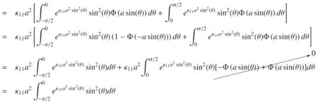
where Φ(.) is standard normal cumulative distribution function. Hence, we get

$$\begin{array}{l}\text{E}\left[e^{j\mathrm{\Delta }\phi (t)}\right]=\frac{4}{\mathit{det}({\mathbf{K}}_{\mathbf{z}})\pi }{\int }_{-\pi /2}^{\pi /2}sin(\theta ){\int }_0^{\infty }{A}_2(t)e^{-{\kappa }_{22}{A}_2^2(t)}\left[\frac{1}{2{\kappa }_{11}}+e^{\frac{{\kappa }_{12}^2{A}_2^2(t){sin}^2(\theta )}{{\kappa }_{11}}}\frac{{\kappa }_{12}{A}_2(t)sin(\theta )\sqrt{\pi }}{{\kappa }_{11}\sqrt{{\kappa }_{11}}}\mathrm{\Phi }\left(-\frac{{\kappa }_{12}{A}_2(t)sin(\theta )}{{\kappa }_{11}}\right)\right]{dA}_2(t)d\theta \\ =\frac{4}{{\kappa }_{12}\sqrt{{\kappa }_{11}\pi }\mathit{det}({\mathbf{K}}_{\mathbf{z}})}{\int }_0^{\infty }{e}^{-{\kappa }_{22}{A}_2^2(t)}\underset{\triangleq C(A_2(t),{\kappa }_{11},{\kappa }_{12})}{\underbrace{{\int }_{-\pi /2}^{\pi /2}{e}^{\frac{{\kappa }_{12}^2{A}_2^2(t){sin}^2(\theta )}{{\kappa }_{11}}}\frac{{\kappa }_{12}^2{A}_2^2(t){sin}^2(\theta )}{{\kappa }_{11}}\mathrm{\Phi }\left(-\frac{{\kappa }_{12}{A}_2(t)sin(\theta )}{{\kappa }_{11}}\right)d\theta }}{dA}_2(t)\end{array}$$ (55)

By defining $a\triangleq -\frac{{\kappa }_{12}{A}_2(t)}{{\kappa }_{11}}$ we simplify C(A₂(t), κ₁₁, κ₁₂):

$$C(A_2(t),{\kappa }_{11},{\kappa }_{12})={\kappa }_{11}{\int }_{-\pi /2}^{\pi /2}{e}^{{\kappa }_{11}{a}^2{sin}^2(\theta )}(a^2{sin}^2(\theta ))\mathrm{\Phi }(asin(\theta ))d\theta$$ (56)

(57)

$${\kappa }_{11}{a}^2\frac{\pi }{4}{e}^{\frac{{\kappa }_{11}{a}^2}{2}}\left[I_0\left(\frac{{\kappa }_{11}{a}^2}{2}\right)+I_1\left(\frac{{\kappa }_{11}{a}^2}{2}\right)\right]$$ (58)

$$=\frac{\pi {\kappa }_{12}^2{A}_2^2(t)}{4{\kappa }_{11}}{e}^{\frac{{\kappa }_{12}^2{A}_2^2(t)}{2{\kappa }_{11}}}\left[I_0\left(\frac{{\kappa }_{12}^2{A}_2^2(t)}{2{\kappa }_{11}}\right)+I_1\left(\frac{{\kappa }_{12}^2{A}_2^2(t)}{2{\kappa }_{11}}\right)\right]$$ (59)

Hence,

$$\text{E}\left[e^{j\mathrm{\Delta }\phi (t)}\right]=\frac{\sqrt{\pi }{\kappa }_{12}}{\underset{\triangleq D}{\underbrace{\mathit{det}({\mathbf{K}}_{\mathbf{z}}){\kappa }_{11}^{3/2}}}}{\int }_0^{\infty }{A}_2^2(t)e^{-{\kappa }_{22}{A}_2^2(t)+\frac{{\kappa }_{12}^2{A}_2^2(t)}{2{\kappa }_{11}}}\left[I_0\left(\frac{{\kappa }_{12}^2{A}_2^2(t)}{2{\kappa }_{11}}\right)+I_1\left(\frac{{\kappa }_{12}^2{A}_2^2(t)}{2{\kappa }_{11}}\right)\right]{dA}_2(t)$$ (60)

$$=D{\int }_0^{\infty }{A}_2^2(t)e^{-A_2^2(t)d}\left[I_0\left({cA}_2^2(t)\right)+I_1\left({cA}_2^2(t)\right)\right]{dA}_2(t)$$ (61)

where $d\triangleq {\kappa }_{22}-\frac{{\kappa }_{12}^2}{2{\kappa }_{11}}$ and $c\triangleq \frac{{\kappa }_{12}^2}{2{\kappa }_{11}}$. Then,

$$\text{E}\left[e^{j\mathrm{\Delta }\phi (t)}\right]=D\left[{\int }_0^{\infty }{A}_2^2(t)e^{-A_2^2(t)d}{I}_0\left({cA}_2^2(t)\right){dA}_2(t)+{\int }_0^{\infty }{A}_2{(t)}^2{e}^{-A_2^2(t)d}{I}_1\left({cA}_2^2(t)\right){dA}_2(t)\right]$$ (63)

Using Mathematica to solve the two integrals in Equ 63 we find:

$$\text{E}\left[e^{j\mathrm{\Delta }\phi (t)}\right]=D\left[{{}_{2}F}_1\left(\frac{3}{4},\frac{5}{4},1,\frac{c^2}{d^2}\right)\frac{\sqrt{\pi }}{4d^{3/2}}+{{}_{2}F}_1\left(\frac{5}{4},\frac{7}{4},2,\frac{c^2}{d^2}\right)\frac{3c\sqrt{\pi }}{16d^{5/2}}\right]$$ (64)

$$=\frac{\pi }{\sqrt{2}{\kappa }_{12}^2\mathit{det}({\mathbf{K}}_{\mathbf{z}})}\left[w^{3/2}{{}_{2}F}_1\left(\frac{3}{4},\frac{5}{4},1,w^2\right)+\frac{3}{4}{w}^{5/2}{{}_{2}F}_1\left(\frac{5}{4},\frac{7}{4},2,w^2\right)\right]$$ (65)

where $w=\frac{{\kappa }_{12}^2}{2{\kappa }_{11}{\kappa }_{22}-{\kappa }_{12}^2}$ and ₂F₁ represents a hypergeometric function. Hence, we get

$$\left|\text{E}\left[e^{j\mathrm{\Delta }\phi (t)}\right]\right|=\left|\frac{\pi }{\sqrt{2}}\left(1-\frac{{\kappa }_{11}{\kappa }_{22}}{{\kappa }_{12}^2}\right)\left[w^{3/2}{{}_{2}F}_1\left(\frac{3}{4},\frac{5}{4},1,w^2\right)+\frac{3}{4}{w}^{5/2}{{}_{2}F}_1\left(\frac{5}{4},\frac{7}{4},2,w^2\right)\right]\right|.$$ (66)

References

- Amor F, Rudrauf D, Navarro V, Ndiaye K, Garnero L, Martinerie J, Le Van Quyen M. Imaging brain synchrony at high spatiotemporal resolution: application to meg signals during absence seizures. Signal processing. 2005;85:2101–2111. [Google Scholar]
- Aviyente S, Bernat E, Evans W, Sponheim S. A phase synchrony measure for quantifying dynamic functional integration in the brain. Human brain mapping. 2010;32:80–93. doi: 10.1002/hbm.21000. [DOI] [PMC free article] [PubMed] [Google Scholar]
- Baillet S, Mosher J, Leahy R. Electromagnetic brain mapping. Signal Processing Magazine, IEEE. 2001;18:14–30. [Google Scholar]
- Bhattacharya J, Petsche H, Feldmann U, Rescher B. Eeg gamma-band phase synchronization between posterior and frontal cortex during mental rotation in humans. Neuroscience Letters. 2001;311:29–32. doi: 10.1016/s0304-3940(01)02133-4. [DOI] [PubMed] [Google Scholar]
- Bressler S. Large-scale cortical networks and cognition. Brain Research Reviews. 1995;20:288–304. doi: 10.1016/0165-0173(94)00016-i. [DOI] [PubMed] [Google Scholar]
- Bressler S, Coppola R, Nakamura R. Episodic multiregional cortical coherence at multiple frequencies during visual task performance. Nature. 1993;366:153–156. doi: 10.1038/366153a0. [DOI] [PubMed] [Google Scholar]
- Bressler S, Ding M, Yang W. Investigation of cooperative cortical dynamics by multivariate autoregressive modeling of event-related local field potentials. Neurocomputing. 1999;26:625–631. [Google Scholar]
- Brovelli A, Ding M, Ledberg A, Chen Y, Nakamura R, Bressler S. Beta oscillations in a large-scale sensorimotor cortical network: directional influences revealed by granger causality. Proceedings of the National Academy of Sciences of the United States of America. 2004;101:9849. doi: 10.1073/pnas.0308538101. [DOI] [PMC free article] [PubMed] [Google Scholar]
- Canolty R, Cadieu C, Koepsell K, Ganguly K, Knight R, Carmena J. Detecting event-related changes of multivariate phase coupling in dynamic brain networks. Journal of neurophysiology. 2012;107:2020–2031. doi: 10.1152/jn.00610.2011. [DOI] [PMC free article] [PubMed] [Google Scholar]
- Celka P. Statistical analysis of the phase-locking value. Signal Processing Letters, IEEE. 2007;14:577–580. [Google Scholar]
- Challis R, Kitney R. Biomedical signal processing (in four parts) Medical and Biological Engineering and Computing. 1991;29:1–17. doi: 10.1007/BF02446290. [DOI] [PubMed] [Google Scholar]
- Davenport W, Root W. An introduction to the theory of random signals and noise. Vol. 11. McGraw-Hill; New York: 1958. [Google Scholar]
- David O, Garnero L, Cosmelli D, Varela F. Estimation of neural dynamics from meg/eeg cortical current density maps: application to the reconstruction of large-scale cortical synchrony. Biomedical Engineering, IEEE Transactions on. 2002;49:975–987. doi: 10.1109/TBME.2002.802013. [DOI] [PubMed] [Google Scholar]
- Ding M, Bressler S, Yang W, Liang H. Short-window spectral analysis of cortical event-related potentials by adaptive multivariate autoregressive modeling: data preprocessing, model validation, and variability assessment. Biological cybernetics. 2000;83:35–45. doi: 10.1007/s004229900137. [DOI] [PubMed] [Google Scholar]
- Doesburg S, Roggeveen A, Kitajo K, Ward L. Large-scale gamma-band phase synchronization and selective attention. Cerebral Cortex. 2008;18:386–396. doi: 10.1093/cercor/bhm073. [DOI] [PubMed] [Google Scholar]
- Gallager R. Circularly-symmetric gaussian random vectors. 2008:1–9. preprint. [Google Scholar]
- Guevara R, Velazquez J, Nenadovic V, Wennberg R, Senjanović G, Dominguez L. Phase synchronization measurements using electroencephalographic recordings. Neuroinformatics. 2005;3:301–313. doi: 10.1385/NI:3:4:301. [DOI] [PubMed] [Google Scholar]
- Horwitz B. The elusive concept of brain connectivity. Neuroimage. 2003;19:466–470. doi: 10.1016/s1053-8119(03)00112-5. [DOI] [PubMed] [Google Scholar]
- Hurtado J, Rubchinsky L, Sigvardt K. Statistical method for detection of phase-locking episodes in neural oscillations. Journal of neurophysiology. 2004;91:1883–1898. doi: 10.1152/jn.00853.2003. [DOI] [PubMed] [Google Scholar]
- Jammalamadaka S, Sengupta A. Topics in circular statistics. Vol. 5. World Scientific Pub Co Inc; 2001. [Google Scholar]
- Klein A, Sauer T, Jedynak A, Skrandies W. Conventional and wavelet coherence applied to sensory-evoked electrical brain activity. Biomedical Engineering, IEEE Transactions on. 2006;53:266–272. doi: 10.1109/TBME.2005.862535. [DOI] [PubMed] [Google Scholar]
- Lachaux J, Chavez M, Lutz A. A simple measure of correlation across time, frequency and space between continuous brain signals. Journal of neuroscience methods. 2003;123:175–188. doi: 10.1016/s0165-0270(02)00358-8. [DOI] [PubMed] [Google Scholar]
- Lachaux J, Rodriguez E, Martinerie J, Varela F, et al. Measuring phase synchrony in brain signals. Human brain mapping. 1999;8:194–208. doi: 10.1002/(SICI)1097-0193(1999)8:4<194::AID-HBM4>3.0.CO;2-C. [DOI] [PMC free article] [PubMed] [Google Scholar]
- Lachaux J, Rodriguez E, MICHEL L, ANTOINE L, Martinerie J, FRANCISCO J. Studying single-trials of phase synchronous activity in the brain. International Journal of Bifurcation and Chaos. 2000;10:2429–2439. [Google Scholar]
- Lancaster H, Seneta E. Chi-Square Distribution. Wiley Online Library; 2005. [Google Scholar]
- Le Van Quyen M, Foucher J, Lachaux J, Rodriguez E, Lutz A, Martinerie J, Varela F. Comparison of hilbert transform and wavelet methods for the analysis of neuronal synchrony. Journal of neuroscience methods. 2001;111:83–98. doi: 10.1016/s0165-0270(01)00372-7. [DOI] [PubMed] [Google Scholar]
- Liang H, Ding M, Bressler S. Temporal dynamics of information flow in the cerebral cortex. Neurocomputing. 2001;38:1429–1435. [Google Scholar]
- Mima T, Matsuoka T, Hallett M. Functional coupling of human right and left cortical motor areas demonstrated with partial coherence analysis. Neuroscience letters. 2000;287:93–96. doi: 10.1016/s0304-3940(00)01165-4. [DOI] [PubMed] [Google Scholar]
- Mormann F, Lehnertz K, David P, Elger EC. Mean phase coherence as a measure for phase synchronization and its application to the eeg of epilepsy patients. Physica D: Nonlinear Phenomena. 2000;144:358–369. [Google Scholar]
- Nolte G, Bai O, Wheaton L, Mari Z, Vorbach S, Hallett M, et al. Identifying true brain interaction from eeg data using the imaginary part of coherency. Clinical Neurophysiology. 2004;115:2292–2307. doi: 10.1016/j.clinph.2004.04.029. [DOI] [PubMed] [Google Scholar]
- Nunez P, Srinivasan R, Westdorp A, Wijesinghe R, Tucker D, Silberstein R, Cadusch P. Eeg coherency:: I: statistics, reference electrode, volume conduction, laplacians, cortical imaging, and interpretation at multiple scales. Electroencephalography and clinical Neurophysiology. 1997;103:499–515. doi: 10.1016/s0013-4694(97)00066-7. [DOI] [PubMed] [Google Scholar]
- Ossadtchi A, Greenblatt R, Towle V, Kohrman M, Kamada K. Inferring spatiotemporal network patterns from intracranial eeg data. Clinical Neurophysiology. 2010;121:823–835. doi: 10.1016/j.clinph.2009.12.036. [DOI] [PMC free article] [PubMed] [Google Scholar]
- Quiroga R, Kraskov A, Kreuz T, Grassberger P. Performance of different synchronization measures in real data: a case study on electroencephalographic signals. Physical Review E. 2002;65:041903. doi: 10.1103/PhysRevE.65.041903. [DOI] [PubMed] [Google Scholar]
- Rudrauf D, Douiri A, Kovach C, Lachaux J, Cosmelli D, Chavez M, Adam C, Renault B, Martinerie J, Le Van Quyen M. Frequency flows and the time-frequency dynamics of multivariate phase synchronization in brain signals. Neuroimage. 2006;31:209–227. doi: 10.1016/j.neuroimage.2005.11.021. [DOI] [PubMed] [Google Scholar]
- Schelter B, Winterhalder M, Dahlhaus R, Kurths J, Timmer J. Partial phase synchronization for multivariate synchronizing systems. Physical review letters. 2006;96:208103. doi: 10.1103/PhysRevLett.96.208103. [DOI] [PubMed] [Google Scholar]
- Stam C, Nolte G, Daffertshofer A. Phase lag index: assessment of functional connectivity from multi channel eeg and meg with diminished bias from common sources. Human brain mapping. 2007;28:1178–1193. doi: 10.1002/hbm.20346. [DOI] [PMC free article] [PubMed] [Google Scholar]
- Swets J. Signal detection theory and ROC analysis in psychology and diagnostics: Collected papers. Lawrence Erlbaum Associates, Inc; 1996. [Google Scholar]
- Tass P, Rosenblum M, Weule J, Kurths J, Pikovsky A, Volkmann J, Schnitzler A, Freund H. Detection of n: m phase locking from noisy data: application to magnetoencephalography. Physical Review Letters. 1998;81:3291–3294. [Google Scholar]
- Tononi G, Edelman G. Consciousness and complexity. Science. 1998;282:1846–1851. doi: 10.1126/science.282.5395.1846. [DOI] [PubMed] [Google Scholar]
- Varela F, Lachaux J, Rodriguez E, Martinerie J. The brainweb: phase synchronization and large-scale integration. Nature reviews neuroscience. 2001;2:229–239. doi: 10.1038/35067550. [DOI] [PubMed] [Google Scholar]
- Vinck M, Oostenveld R, van Wingerden M, Battaglia F, Pennartz C. An improved index of phase-synchronization for electrophysiological data in the presence of volume-conduction, noise and sample-size bias. Neuroimage. 2011;55:1548–1565. doi: 10.1016/j.neuroimage.2011.01.055. [DOI] [PubMed] [Google Scholar]
- Vinck M, Van Wingerden M, Womelsdorf T, Fries P, Pennartz C. The pairwise phase consistency: a bias-free measure of rhythmic neuronal synchronization. Neuroimage. 2010;51:112–122. doi: 10.1016/j.neuroimage.2010.01.073. [DOI] [PubMed] [Google Scholar]
- Vo A, Oraintara S, Nguyen N. Vonn distribution of relative phase for statistical image modeling in complex wavelet domain. Signal Processing. 2011;91:114–125. [Google Scholar]
- Whittaker J. Graphical models in applied multivariate statistics. Wiley Publishing; 2009. [Google Scholar]