A Time to Event Tutorial for Pharmacometricians

Models for time to event provide the link between standard pharmacokinetic–dynamic models disease progression, and clinical outcome events. The biological basis for events may be expressed quantitatively in terms of a hazard function. This tutorial explains hazards and how doses can be linked to events predicted from hazard functions.

Overview

This tutorial is intended for pharmacometricians with a good grounding in the basic concepts of pharmacokinetics, pharmacodynamics, and population modeling.¹ It links these concepts to the principles of time-to-event (TTE) analysis. The idea of the hazard is essential to understand why and when events occur. Simple mathematical operations convert the hazard into quantities such as the survivor function and likelihood that are useful for graphical representation and parameter estimation. The ideas will be explained using statistical and mathematical theory only to the extent necessary to understand the quantitative applications to clinical pharmacology. An excellent guide to the statistical aspects of survival analysis can be found in Collett's textbook.² A more light-hearted historical view can be found in chapter 7 of Senn's book.³

The Hazard: The Biological Basis of Survival

What is an event?

Events are things that happen at a particular time. The traditional biomedical example of an event is death. The description of the times of death in a population is known as survival analysis and has been the motivating factor for statistical theory and methodology. More generally, the description of event times is called TTE analysis. Death (except in cats) occurs only once for an individual, but there are many other kinds of biomedical events that may occur more than once, e.g., epileptic seizures, myocardial infarctions, bone fractures, and kidney transplant rejections.

The description of multiple events in an individual is called repeated TTE analysis. If many events occur in the same individual, then the average of the number of events over a convenient interval is described by the event frequency, e.g., epileptic seizures and episodes of angina pain. Although these frequency measures are simple to understand, the underlying biological and pharmacological basis for predicting the frequency may be concealed by ignoring the time of each event and only recording the number of events. An additional aspect of an event is that it may be associated with a severity score that may be combined with a model for the frequency of events.⁴ This tutorial will confine itself to models for single events.

Why and when do events happen?

Why events happen is often poorly understood, but there are two main mechanisms that might be considered. An event such as death is typically related to the things that have happened throughout life. It is the cumulative effect of living that can be used to predict the time to death. On the other hand, death may occur without any obvious connection to previous lifestyle, e.g., being struck by lightning (although that will be more common in those who live more in the outdoors). Such apparently random times of events can be described in terms of frequency by distributions such as the Poisson distribution, but because they are random, they are not very interesting from the viewpoint of understanding biology, disease, and the influence of medical treatment. This tutorial focuses on those kind of events that are predictable from things happening before the event.

Pharmacokinetics and survival: biological brothers

The bread and butter of pharmacometrics is the science of pharmacokinetics. In the simplest case, the time course of drug disappearance from the body may be described by an elimination rate constant. The elimination rate constant (k) defines the relationship between the amount of drug in the body and the instantaneous rate of elimination (Eq. 1).

There is an exact parallel between this well-known equation and the basic equation of survival analysis (Eq. 2).

The number of people alive corresponds to the amount of drug in the body (which is directly proportional to the number of molecules still in the body). The number of people dying corresponds to the rate of elimination (which is directly proportional to the number of molecules being lost (“killed”)).

The elimination rate constant, k, is simply the proportionality constant connecting amount to elimination. In the number dying expression (Eq. 2), the constant h is the hazard. It has exactly the same meaning as k in the rate of elimination expression (Eq. 1)—the proportionality constant relating people who are alive to the death rate. Understanding what the hazard means is at the heart of TTE analysis.

Hazards, exactly like elimination rate constants, have units of 1/time. Death rates are usually reported in a standardized way, e.g., deaths per 100,000 people alive, but this is just for convenience of representing the numerical value. If the death rate was standardized per person alive, then this would be the value of the hazard.

Pharmacokineticists who understand the properties of elimination rate constants should soon feel comfortable with hazards. The simplest elimination mechanism for drug molecules is first order in which the elimination rate constant does not change. In terms of death rate (“elimination rate”), the simplest case occurs with a constant hazard (first-order dying).

To predict the time course of amount of drug (A(t)) in the body, the elimination rate can be integrated that leads to an exponential equation (Eq. 3) with an initial amount A0:

The same form of equation (Eq. 4) predicts survival, Sn(t), where the survival has an initial value (S0) representing the number of people alive at time 0.

The time course of the probability of survival, S(t), is called the survivor function when the value of S0 is standardized to one person.

This simple product of hazard h and time t to predict the survivor function in Eq. 4 only works when the hazard is constant.

More generally, the survivor function is calculated from the integral of the hazard with respect to time—a quantity called the cumulative hazard (cumhaz) as shown in Eq. 5.

The cumulative hazard is sometimes known as the risk. Although the term risk is widely used in daily life, it does not have a clearly accepted meaning in the TTE analysis literature.

In this example, it should be clear that the pharmacokinetic elimination rate constant in a pharmacokinetic model is identical to the hazard in a survivor function model. Both the rate constant and the hazard have dimensions of 1/time and can be interpreted to have the same meaning.

Despite the name, the elimination rate constant may not be constant. Indeed, it may change due to a variety of factors, e.g., with concentration if elimination is mixed order. Code illustrating models for the amount in the body is shown in Eq. 6 using a pharmacokinetic model and in Eq. 7 using a survival model.

The code shows what seem to be quite different approaches to calculate either the amount or the survival. Yet both approaches give identical results for first-order or mixed-order elimination (Supplementary Table S1 and Supplementary Data online).

The likelihood of observing an event at a particular time is predicted by the probability density function (pdf). When the exact time of the event is observed, the likelihood is the product of the survivor function and the hazard at that time (Eq. 8).

In general, the pdf for the distribution of survival times is obtained from the product of the survivor function and the hazard. When the hazard is constant, the shape of the pdf is exponential. This is because the exponential survivor function shape does not change when multiplied by the constant hazard. In this special case of a constant hazard, the event times are described as having an exponential distribution.

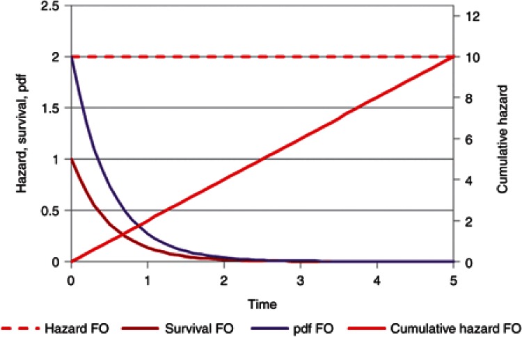
A TTE view of a drug with first-order elimination illustrates the hazard (rate constant), cumulative hazard, survivor function (amount/initial dose), and pdf (Figure 1). By definition, the rate constant with first-order elimination is constant over time. The cumulative hazard increases linearly with time and the survivor function, which corresponds to the amount of drug remaining divided by the dose, decreases exponentially as expected for amount in the body. The likelihood of a molecule being eliminated at a particular time is described by the pdf.

Figure 1.

First-order (FO) elimination is the same as a constant baseline hazard. The hazard, cumulative hazard, survivor function (survival), and probability density function (pdf) are shown. The survivor function is equivalent to the amount but standardized to the initial dose.

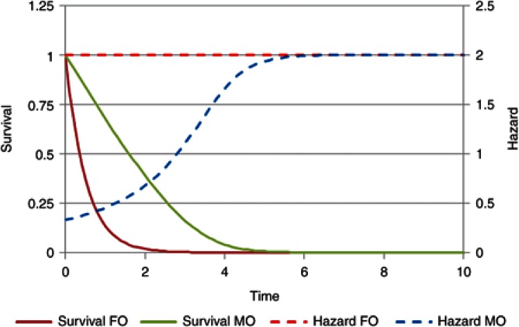
A comparison of the hazard and survivor function for drugs with either first-order or mixed-order elimination is shown in Figure 2. In this example, the mixed-order elimination process reaches half of its maximum capacity when the survivor function is 0.1 (Km). The hazard for mixed-order elimination is equivalent to the rate constant for elimination at a particular amount remaining. The survivor function starts at 10 times the Km with a hazard of 0.33 as compared with the first-order hazard of 2. As the amount left in the body approaches zero, the hazard for the mixed-order process approaches the first-order value (after time unit 5).

Figure 2.

The hazard (rate constant) and survivor function (amount/dose) for first-order elimination (FO) and mixed-order (MO) elimination.

TTE distributions

The simplest TTE distribution is the exponential distribution that arises when the hazard is constant. A family of exponential hazard models are obtained from extensions to the constant hazard case summarized in Supplementary Table S2 online. When the hazard increases with time, this may be expressed with the Gompertz function (Eq. 9). Gompertz is considered as the father of survival analysis, and he called this function the “law of mortality” when it was published in 1825.⁵ The corresponding event time distribution is called the Gompertz distribution.

The Weibull hazard function is often written as shown in Eq. 10:

But may also be written with a different parameterization as shown in Eq. 11:

This hazard is exactly equivalent but shows more clearly the relationship to other exponential hazard functions (Supplementary Table S2 online). The resulting TTE distribution is called the Weibull distribution. The Weibull hazard function (Eq. 10) requires some care because when time is zero, the hazard is zero, but this cannot be computed from the usual functions (ln(0) or 0^γ−1). In practice, Eq. 11 should only be used when t > 0. When t = 0, the Weibull hazard is 0. It is debatable what biological meaning can be attached to a hazard of zero. In real life, the time of zero is at entry into a clinical study, and it is unrealistic to imagine that at exactly that instant, the hazard of an event such as death plunges to zero.

When there are no time-varying covariates involved, there is often an analytical solution to obtain the cumulative hazard (e.g., the Weibull), and from that, it is easy to predict the survivor function and the pdf. These simple cases (with others such as log normal and log logistic) are the standard survival distribution choices available in common statistical software. For more flexible hazard functions involving time-varying covariates, these analytical solutions are not usually available. With software that is able to numerically integrate the hazard function, there is no restriction on the way the hazard is expressed except the user needs to ensure that the hazard does not go negative. If the hazard is negative, this gives rise to the Lazarus distribution, which has been predicted⁶ but not yet observed. The exponential forms of the hazard are useful because they avoid negative hazards as long as λ₀ is not negative. The generalized exponential hazard (e.g., Eq. 12) may have any function in the exponential term.

Other forms of the hazard that do not use an exponential may be more convenient, but the exponential form has an advantage for interpretation of the parameters in the exponent.

Eq. 13 includes a parameter β_SEX and a SEX covariate (female = 0 and male = 1). The value of β_SEX is easily interpreted by exponentiation. If the value of β_SEX is 0.693, then exp(0.693 × 0) for women is 1 and exp(0.693 × 1) for men is 2. The hazard for men is 2 relative to women. This is called the hazard ratio. In real life, the male hazard ratio changes with age (e.g., see page 139 in ref. ³ with a value of 2 around the age of 20 years and again at 30 years in a UK population).

The power of the hazard function becomes evident in pharmacometric applications when factors changing the hazard vary with time. An obvious example would be if drug treatment influenced the hazard. The effects of the drug will depend on concentration and thus, the hazard in the drug-treated arm will vary with the time course of drug concentration.

A series of simulations are used to demonstrate the concepts of hazard, cumulative hazard, survival, and likelihood of an event by comparing what might be observed in a placebo-controlled trial of a drug that reduces the hazard.

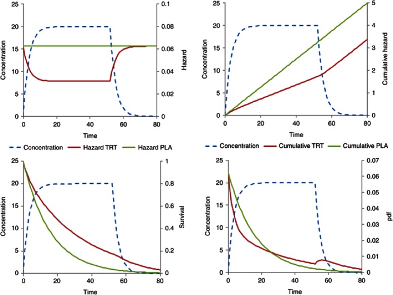
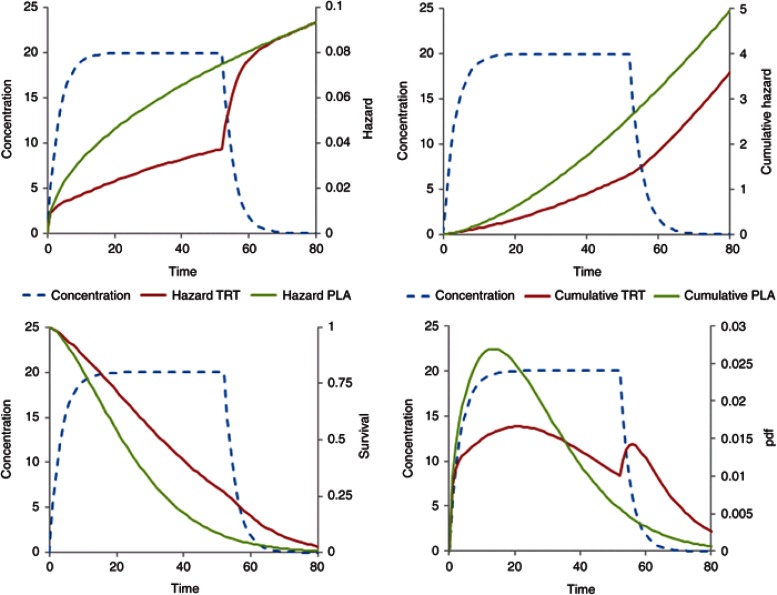
Figure 3 illustrates a constant baseline hazard in the placebo arm. The drug effect on the baseline hazard, λ₀, is assumed to be linearly related to concentration, C(t), with a proportionality constant β_C (Eq. 14). For a treatment effect that reduces the hazard, the sign of β_C is negative. As noted above, the user must take care that this does not lead to a negative hazard, e.g., by using an E_max model with E_max constrained to be not greater than −1.

Figure 3.

Constant baseline hazard with time-varying drug effect linearly related to concentration. Treatment starts at time = 0 and stops at time = 52. Plots show the time course of concentration, hazard, cumulative hazard, survivor function (survival), and probability density function (pdf).

For simplicity, the drug input rate is assumed to be constant with concentration approaching steady state after 10 time units. The drug washes out over a similar period when treatment is stopped at time 52. The cumulative hazard reflects the total number of events with a decreased number of events in the drug treatment arm. When treatment has washed out, the cumulative hazard curve is parallel in both the groups. This pattern is similar to a disease-modifying effect of drug treatment on a linear disease progression model.⁷ The survivor function for the placebo arm is exponential but deviates from this shape for the drug treatment arm during treatment wash-in and washout. The likelihood of observing an event as a function of time is shown in the pdf plot. Note the transient increased likelihood of an event after stopping treatment. This might be interpreted as a form of rebound, but the cumulative hazard plot shows that the cumulative number of new events is approximately the same in both the groups. This increase in the pdf is inevitable because the hazard increases as drug concentration washes out so the likelihood of having an event in the previously drug-treated group must increase albeit transiently.

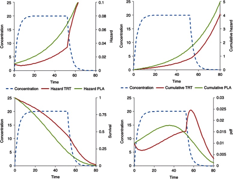
A similar series of plots is shown for a baseline Gompertz hazard function (Figure 4). The exponential increase in hazard in the placebo arm is clearly different from the constant hazard in Figure 3. The treatment effect uses the same pharmacodynamic model and the same value for β_C with an increasing reduction in hazard (Eq. 15). Note that the likelihood (pdf plot) of observing an event in the placebo arm increases with time then drops. This is quite different from the constant hazard likelihood that decreases monotonically. There is a very marked “rebound” in the likelihood of an event after stopping treatment, but no excess of events in the cumulative hazard plot.

Figure 4.

Gompertz baseline hazard with time-varying drug effect linearly related to concentration. Treatment starts at time = 0 and stops at time = 52. Plots show the time course of concentration, hazard, cumulative hazard, survivor function (survival), and probability density function (pdf).

When a Weibull baseline hazard is assumed with the same drug effect (Eq. 16), the shape of the hazard is again quite different (Figure 5).

Figure 5.

Weibull baseline hazard with time-varying drug effect linearly related to concentration. Treatment starts at time = 0 and stops at time = 52. Plots show the time course of concentration, hazard, cumulative hazard, survivor function (survival), and probability density function (pdf).

Like the Gompertz, the Weibull hazard increases with time, but the slope decreases while the Gompertz increases. The likelihood of an event reaches a peak relatively earlier in the placebo arm, and the apparent rebound in the likelihood is smaller.

These three baseline hazard models (exponential, Weibull, and Gompertz) will have a constant hazard ratio for a unit change in concentration. This is because the parameters of the baseline hazard models do not change with time. The time course of the Gompertz and Weibull likelihoods may represent the biology of tumor metastases. There may be a relatively rapid increase in metastases after initial diagnosis, but the incidence of metastases observed in the surviving population drops quite markedly with time. This means that drug treatments may show an important benefit in reducing events earlier in the disease but with much less benefit later. Drug treatments may be approved based on this marked early benefit, but there may be a poorer justification for continuing use when decreasing benefits are weighed against adverse effects and costs of treatment. The usual assumption is that the magnitude of treatment benefits observed in a clinical trial will continue indefinitely, but this is rather naive if the benefit of treatment is expressed as a constant hazard ratio if in fact it decreases with time. Clinical trials that report hazard ratios almost always report a single value and rarely attempt to investigate if the benefit is sustained over time.

Pharmacometricians who are familiar with covariate model building and time-varying covariates applied to pharmacokinetic parameters, e.g., ref. 1, will be able to apply exactly the same ideas to parameters of the hazard function. The hazard function approach, with numerical integration to obtain the cumulative hazard and the survivor function, removes many of the constraints associated with TTE analysis imposed by standard statistical software.

Biomarkers and clinical outcome

Common approaches to TTE analysis only use the baseline value of an explanatory factor such as age or smoking, but when this factor changes with time, the approach needs to be carefully considered. Age is clearly a factor that changes with time, but it is usually used as a constant baseline age factor for the hazard, and a separate time function (e.g., Gompertz baseline hazard) is used to describe how the hazard changes after adjusting for baseline age. A smoking history, however, will have cumulative effects on outcome, and a baseline smoking history would not describe the hazard as well as one that includes the time course, e.g., pack years of cigarettes increasing and perhaps decreasing. Similar considerations apply when a treatment may change over time, e.g., in terms of dose size or periods of stopping and starting treatment.

For example, an increase in mortality with selegiline treatment was noticed in a randomized comparison of levodopa alone with levodopa plus selegiline in patients with Parkinson's disease.⁸ An exploratory analysis of the use of selegiline in a different cohort of patients receiving a variety of treatments failed to confirm an increase in mortality. Critically, this analysis used an intention-to-treat approach that did not take into account the actual use of selegiline, which included periods on and off treatment.⁹

One of the goals of clinical pharmacology is to link drug dose to clinical benefit. When the benefit of drug treatment is described in terms of a change in the time-to-clinical outcome event, then the link between dose and benefit also involves the time course of a biomarker, which in turn influences the event hazard. The term biomarker is used here in a general sense for any quantity that is linked to drug effect. A biomarker may include drug concentration but is more commonly used to refer to measurements of physiological variables such as blood pressure, serum cholesterol, electroencephalogram frequency, or pathological variables such as tumor size or disease severity. Any of these biomarkers may be used as explanatory variables in a hazard function. If a treatment affects a biomarker, then the biomarker change itself may be sufficient to describe the treatment effect on the clinical outcome.

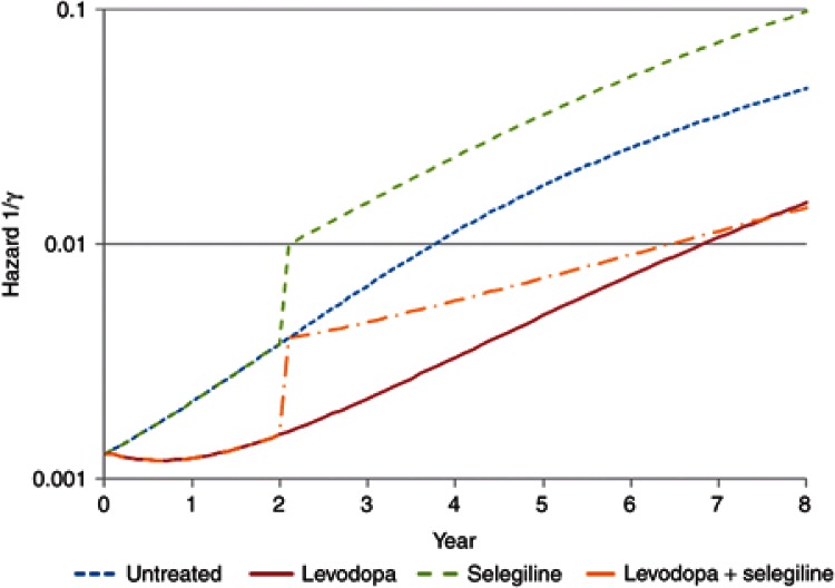
This was shown for the effect of levodopa on mortality in Parkinson's disease when the time course of disease status was used as the biomarker. Treatment with levodopa is associated with an improvement in disease status^10,11 and a decrease in mortality.¹² By contrast, selegiline has also been shown to improve disease status, but after accounting for the effect of disease status progression, there was an independent increase in mortality associated with selegiline.¹² Simply using selegiline treatment in the analysis showed no significant effect on mortality,¹³ but this result is confounded by the beneficial effects on mortality arising from improved disease status caused by selegiline. Selegiline alone has a higher hazard of death because it has a relatively small symptomatic and disease-modifying effect on disease status, which is insufficient to offset the independent effect that increases the hazard. A combination of levodopa and selegiline has a higher hazard than untreated patients, but after about 1.5 years, the hazard of death is lower as compared with untreated patients.¹²

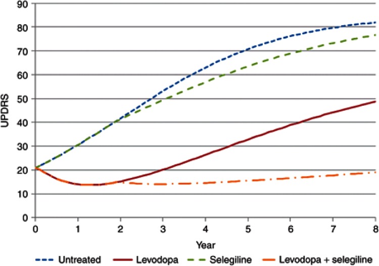
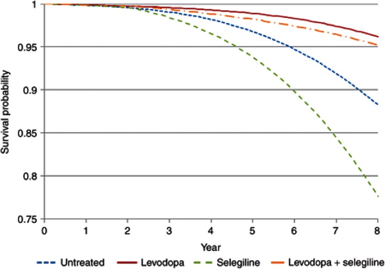
Simulations linking disease progression with effects of drug treatments on progress and hazard allow different treatment strategies to be understood. This is a special opportunity for pharmacometrics to bring an integrated approach to understand the link between dose and outcome. For example, an alternative strategy for the treatment of Parkinson's disease would be to delay treatment with selegiline until levodopa has produced a substantial symptomatic and disease-modifying effect at approximately 2 years. The effect of such a strategy on the time course of disease status in untreated patients, those treated with levodopa alone, and then in combination with selegiline is shown in Figure 6. The predicted hazard of death (Figure 7) for patients with Parkinson's disease shows the benefits of this delayed start of selegiline treatment in reducing mortality (Figure 8). If treatment with selegiline is started 2 years after levodopa, then there is only a small increase in mortality compared with an untreated patient, but the substantial additional disease-modifying benefits of selegiline obtained with levodopa lead to overall better function and, eventually after 6 years of selegiline, a lower hazard of mortality than levodopa alone (Figure 7). This kind of understanding of the link between disease progress, treatment effects on disease status, and consequent effects on mortality cannot be understood from time invariant hazard ratios. It is unlikely that any clinical trial would ever prospectively test this strategy with selegiline. Simulation based on pharmacological understanding can help guide decisions that cannot be made with traditional clinical trial results.

Figure 6.

The time course of Unified Parkinson's Disease Rating Scale (UPDRS) in Parkinson's disease showing effects of treatment with levodopa and selegiline on disease status.

Figure 7.

Hazard of death in Parkinson's disease with levodopa and selegiline.

Figure 8.

Survival probability in Parkinson's disease with levodopa and selegiline.

The missing data problem

It is usually the case that the time of an event is not observed in all subjects. This can happen for two quite different reasons.

If a subject is not followed up long enough, then the event is never observed. This is because the subject drops out from the trial before its end or the trial finishes at some predefined time. This kind of missing event time is called right censored because if one were to imagine a distribution of event times, then the right hand end of the distribution is truncated at the end of a trial. The same term is applied to data that is missing when subjects drop out from a trial.

The other kind of missing data is due to the exact time of the event not being known. For example, the time of death is usually only recorded in clinical trials on the day of death, and the clock time when death was pronounced is not recorded. Therefore, the exact time of the event is not known except that it occurred in a 24-h interval. This kind of missing data is known as interval censored. All TTE data is subject to some degree of interval censoring, which is often ignored if the time interval in which the event occurs is short. The time of dropout from a clinical trial is itself of interest for TTE analysis. Quite commonly, the time of dropout is not known because subjects may be seen at one visit and then not appear at the next scheduled time. In this case, the interval containing the actual time of dropout may be quite long, e.g., several weeks or months.

Estimation of the parameters of a hazard function using maximum likelihood methods uses the likelihood of an event at an exact time, or within a known interval with interval censoring or after a known time due to right censoring. The likelihoods of these three possibilities are obtained simply from the survivor function and the hazard (Supplementary Table S3 online).

An informative application of interval censoring is described by Hu and Sale¹⁴ who link the concepts of a time-varying hazard of dropout to estimation of the hazard function when event times are censored. Using the predicted time course of progression in a joint model of disease status and time to drop out, they were able to show that dropouts may not occur completely at random but depend on the time course of disease progression. They also demonstrated that using the last disease status, observation carried forward as a covariate for the dropout hazard function did not describe the dropout time distribution as well as using the predicted progress of the disease.

Estimation and diagnostics

Algorithms for obtaining initial estimates of the survivor function and the hazard function are described in Collett,² and software may be found at http://cran.r-project.org/web/views/Survival.html. The density of the TTE data is usually rather low and this may make it difficult to interpret the shape of the hazard function. Equally because the survivor function is a representation of the cumulative hazard, the time course of the hazard is integrated out, and it is hard to glean information about the hazard time course.

Nonlinear mixed-effect modeling packages that are widely used by pharmacometricians (e.g., NONMEM) are easy to use for modeling TTE data.^15,16 The hazard function is written by the user and integrated by the software. The likelihood is then calculated from the cumulative hazard. Parameters included in the hazard function are estimated in the usual way.

Residual based methods of model evaluation are highly subjective and offer no good guidance for understanding the hazard function. Collett² discusses various residual based diagnostics and points out their limitations.

A form of visual predictive check for predictions of the hazard function can be created by comparing a Kaplan–Meier plot with 95% CI from the original data to the simulated median and 95% CI obtained by simulating many replicates of the event time distribution and performing a Kaplan–Meier plot on each replicate.^12,17

In all cases, it is interesting to note that the least informative plot is the survivor function. Although differences between placebo and drug treatment are visible, the changes related to the time course of drug effect are more subtle and would be difficult to observe in nonparametric graphical displays of the survivor function (e.g., the Kaplan–Meier plot) that are commonly used in the biomedical literature.

Conclusion

Pharmacometrics provides the scientific concepts and tools for understanding pharmacology in a quantitative manner. It brings together basic principles of pharmacology with statistical methods to describe and predict the effects of drug treatments. Clinical trials designed to observe outcome events are often expensive in both time and money. TTE analysis informed by pharmacology and physiology can reveal more than what is typically found in published reports. It is hoped that this tutorial will encourage a deeper understanding of how drugs work and improve the way they can change clinical outcome.

Author Contributions

N.H. wrote manuscript.

Conflict of interest

The author declared no conflict of interest.

References

- Mould D.R., Upton R.N. Basic concepts in population modeling, simulation, and model-based drug development. CPT: Pharmacomet. Syst. Pharmacol. 2012;1:e6. doi: 10.1038/psp.2012.4. [DOI] [PMC free article] [PubMed] [Google Scholar]
- Collett D. Modelling Survival Data in Medical Research. 2nd edn. (CRC Press, Boca Raton, FL, USA, 2003); [Google Scholar]
- Senn S. Dicing With Death: Chance, Risk and Health. Cambridge University Press, Cambridge, UK; 2003. [Google Scholar]
- Plan E.L., Karlsson K.E., Karlsson M.O. Approaches to simultaneous analysis of frequency and severity of symptoms. Clin. Pharmacol. Ther. 2010;88:255–259. doi: 10.1038/clpt.2010.118. [DOI] [PubMed] [Google Scholar]
- Gompertz B. On the nature of the function expressive of the law of human mortality, and on a new mode of determining the value of life contingencies. Phil. Trans. R. Soc. London. 1825;115:513–583. doi: 10.1098/rstb.2014.0379. [DOI] [PMC free article] [PubMed] [Google Scholar]
- Wheatley-Price P., Hutton B., Clemons M. The Mayan doomsday's effect on survival outcomes in clinical trials. CMAJ. 2012;184:2021–2022. doi: 10.1503/cmaj.121616. [DOI] [PMC free article] [PubMed] [Google Scholar]
- Chan P.L., Holford N.H. Drug treatment effects on disease progression. Annu. Rev. Pharmacol. Toxicol. 2001;41:625–659. doi: 10.1146/annurev.pharmtox.41.1.625. [DOI] [PubMed] [Google Scholar]
- Lees A.J. Comparison of therapeutic effects and mortality data of levodopa and levodopa combined with selegiline in patients with early, mild Parkinson's disease. Parkinson's Disease Research Group of the United Kingdom. BMJ. 1995;311:1602–1607. doi: 10.1136/bmj.311.7020.1602. [DOI] [PMC free article] [PubMed] [Google Scholar]
- The Parkinson Study Group Mortality in DATATOP: a multicenter trial in early Parkinson's disease. Ann. Neurol. 1998;43:318–325. doi: 10.1002/ana.410430309. [DOI] [PubMed] [Google Scholar]
- Vu T.C., Nutt J.G., Holford N.H. Progression of motor and nonmotor features of Parkinson's disease and their response to treatment. Br. J. Clin. Pharmacol. 2012;74:267–283. doi: 10.1111/j.1365-2125.2012.04192.x. [DOI] [PMC free article] [PubMed] [Google Scholar]
- Holford N.H., Chan P.L., Nutt J.G., Kieburtz K., Shoulson I., Parkinson Study Group Disease progression and pharmacodynamics in Parkinson disease - evidence for functional protection with levodopa and other treatments. J. Pharmacokinet. Pharmacodyn. 2006;33:281–311. doi: 10.1007/s10928-006-9012-6. [DOI] [PubMed] [Google Scholar]
- Vu T.C., Nutt J.G., Holford N.H. Disease progress and response to treatment as predictors of survival, disability, cognitive impairment and depression in Parkinson's disease. Br. J. Clin. Pharmacol. 2012;74:284–295. doi: 10.1111/j.1365-2125.2012.04208.x. [DOI] [PMC free article] [PubMed] [Google Scholar]
- Holford N.H.G., Vu T., Nutt J.Authors' response to Marras & Oakes “Piecing together the puzzle of progression and mortality in Parkinson's disease.” Br J Clin Pharmacol 2012. doi:10.1111/j.1365-2125.2012.04465.x [DOI] [PMC free article] [PubMed]
- Hu C., Sale M.E. A joint model for nonlinear longitudinal data with informative dropout. J. Pharmacokinet. Pharmacodyn. 2003;30:83–103. doi: 10.1023/a:1023249510224. [DOI] [PubMed] [Google Scholar]
- Holford N.H.G., Lavielle M.A tutorial on time to event analysis for mixed effect modellers Abstr 2281. PAGE 202011 ). < http://www.page-meeting.org/?abstract=2281 >. [Google Scholar]
- Holford N.H.G.Time to event analysis for pharmacokineticists. AAPS Webinar < http://holford.fmhs.auckland.ac.nz/docs/time-to-event-webinar.pdf >. ( 2012
- Garnett C., Holford N.H.G. 5th International Symposium on Measurement and Kinetics of In Vivo Drug Effects, Noordwijkerhout, 26–29 April 2006; Bone mineral density progression linked to dropout and time-to-fracture: application to postmenopausal women taking hormone replacement therapy. [Google Scholar]
Associated Data
This section collects any data citations, data availability statements, or supplementary materials included in this article.