Enhanced Localization of Genetic Samples through Linkage-Disequilibrium Correction

Abstract

Characterizing the spatial patterns of genetic diversity in human populations has a wide range of applications, from detecting genetic mutations associated with disease to inferring human history. Current approaches, including the widely used principal-component analysis, are not suited for the analysis of linked markers, and local and long-range linkage disequilibrium (LD) can dramatically reduce the accuracy of spatial localization when unaccounted for. To overcome this, we have introduced an approach that performs spatial localization of individuals on the basis of their genetic data and explicitly models LD among markers by using a multivariate normal distribution. By leveraging external reference panels, we derive closed-form solutions to the optimization procedure to achieve a computationally efficient method that can handle large data sets. We validate the method on empirical data from a large sample of European individuals from the POPRES data set, as well as on a large sample of individuals of Spanish ancestry. First, we show that by modeling LD, we achieve accuracy superior to that of existing methods. Importantly, whereas other methods show decreased performance when dense marker panels are used in the inference, our approach improves in accuracy as more markers become available. Second, we show that accurate localization of genetic data can be achieved with only a part of the genome, and this could potentially enable the spatial localization of admixed samples that have a fraction of their genome originating from a given continent. Finally, we demonstrate that our approach is resistant to distortions resulting from long-range LD regions; such distortions can dramatically bias the results when unaccounted for.

Introduction

Discerning the spatial structure of individuals on the basis of their genetic material has important applications to medical genetics with regard to finding mutations that increase disease risk,^1,2 most notably through facilitating powerful corrections of stratification.³ This task is also crucial for population-genetic studies (e.g., studies of selection,⁴ migration,⁵ and recombination^6,7), which provide insights into human demographics and history.⁸ Moreover, it has recently been shown that ancestry inference is of critical value in pharmacogenomics.⁹

Inferring spatial genetic structure has been traditionally performed via dimensionality-reduction techniques—typically principal-component analysis (PCA)^3–10—which rely on the similarity between geographic maps of population locations and the reduced-dimension maps. Although often successful and conceptually simple, PCA is a generic method that does not directly model any properties that are unique to genetic data. Recently, a method that uses an explicit probabilistic model to describe genetic variation as a function of spatial position has been proposed;¹¹ among the advantages of this model-based approach, named SPA, is its ability to handle genomes of mixed individuals and detect selection signals.

A major drawback of all existing approaches to spatial localization is that they do not model linkage disequilibrium (LD) among markers across the genome. Correlations among markers in the form of LD violate the inherent assumptions made by both PCA and SPA. Intuitively, in the presence of linked markers, each marker is assumed to provide independent evidence of the sample’s origin, although this is not truly the case (for example, a pair of two perfectly linked markers should only be counted as one). The cumulative effect of such unaccounted-for correlations not only decreases accuracy but can also bias the results, even in the presence of an infinite number of samples.¹² Moreover, in addition to containing local LD, the genome contains long-range LD regions in which correlations among variants can extend up to megabases as a result of the suppression of recombination, for instance, after a chromosomal inversion. The effects of these regions are strong enough to dominate the top principal components (PCs) in some data sets. When the bias is obvious, a possible remedy is the removal of the problematic genomic parts;¹³ in less extreme cases, such biases are likely to go undetected, as we demonstrate in the Results.

In this work, we introduce LOCO-LD, an approach to performing spatial localization corrected for LD. LOCO-LD uses a probabilistic model to describe the allele frequencies and the linkage patterns within short genomic windows. Specifically, the genotypes (or haplotypes when the data are phased) within a window are modeled as being sampled from a multivariate normal distribution, and LD is captured through the pairwise correlations between markers. Similarly to SPA, we model allele frequencies as a function of the spatial position. In contrast to existing methods, LOCO-LD is designed primarily to work in a supervised manner by using training data from individuals whose origins are known. Such training data sets, which are becoming widely available, can be leveraged for improving the localization accuracy, as we show in the Results. Given the training genotypes and their origins, we estimate the parameters of the model and localize new individuals through a maximum-likelihood procedure. We derive closed-form formulae for the maximum-likelihood estimators to achieve a fast and robust approach.

We validated our method on large-scale genotype data from a set of 1,385 European individuals with known country of origin from the POPRES data set.¹⁴ First, we show that LOCO-LD performs significantly better than current widely used methods in localizing European individuals; compared with the commonly used PCA approach, which has a localization error of ∼247 km, LOCO-LD has a median localization error of ∼206 km. The key to its success is that whereas PCA and SPA deteriorate as the marker set becomes denser (and as a result, LD increases among markers), LOCO-LD keeps improving. This property is critical, considering recent developments in genotyping and sequencing technologies, which enable genotyping samples over increasingly dense SNP panels.

Second, we show that compared with that of PCA, LOCO-LD’s performance is less sensitive to decreases in the amount of available genomic information. For example, whereas PCA’s localization error increases by ∼80% when only 20% of the genome is utilized, LOCO-LD’s error increases by ∼30%. This suggests LOCO-LD as the method of choice for the localization of single-ancestry segments extracted from the genomes of admixed samples.^5,15 For example, given the genome of an African American individual, the African and European haplotype segments can be accurately retrieved with the use of existing local-ancestry-inference methods.^16,17 Similarly to previous work,¹⁵ LOCO-LD can then be applied to fragments of different local ancestries in order to estimate the separate African and European origins, and its accuracy should remain high despite the fact that only part of the genome is being used for each of the two inference tasks. LOCO-LD is also the best-performing method on very short DNA segments (in the order of megabases) and is therefore likely to perform well when integrated into a local-ancestry-inference method, similarly to existing PCA-based approaches.⁵

Finally, in order to compare the robustness of the different methods to the effects of long-range LD, we apply them to a data set of Spanish individuals, whose relative homogeneity allows for the easy detection of such signals. Indeed, we detected a strong distortion, which we traced back to a common inversion on chromosome 8. Whereas the results of both PCA and SPA were affected, LOCO-LD was resistant to the distortion. We also provide simulations that demonstrate the effects of variously sized long-range LD regions on the accuracy of spatial inference.

Subjects and Methods

LD-Aware Spatial Model

Suppose we have a sample of genotypes over a common set of SNPs and we would like to estimate the geographic locations from which each sample originated (the method works just as well for haplotypes with a slight modification, which we explain later). Suppose also that we have a set of n genotypes, g₁…g_n, whose locations of origin, x₁…x_n (x_i is a d × 1 vector and d is the dimension of the spatial representation), are known to a reasonable precision. We will train a model on these n samples and use the inferred parameters to estimate the locations of the samples whose origins are unknown.

Our model describes the expected genotype value of each SNP across space as a linear function of the position, and in that regard, it is similar to SPA. In addition, we divide the genotypes into nonoverlapping windows of length l and model the pairwise correlations between pairs of SNPs within each window as window specific and constant (position independent). Finally, we assume that the genotypes within a window are sampled from a multivariate normal distribution (MVN). The score function that we obtain for window j is therefore

$$\mathcal{L}\left(g_{1j}\dots g_{nj};{\beta }_j,{\text{Σ}}_j\right)=\prod _{i=1}^n\frac{1}{{\left(2\pi \right)}^{\frac{l}{2}}{\left|{\text{Σ}}_j\right|}^{\frac{1}{2}}}{e}^{-\frac{1}{2}{\left({\beta }_j{x}_i-g_{ij}\right)}^T{\text{Σ}}_j^{-1}\left({\beta }_j{x}_i-g_{ij}\right)},$$ (Equation 1)

where g_ij is an l × 1 vector containing the portion of genotype i restricted to window j, β_j is an l × d linear-coefficient matrix describing the position-dependent allele frequencies in the window, and Σ_j is the l × l matrix of pairwise correlations within the window.

The MVN is not a natural choice for describing discrete genotypes; ideally, we would use a discrete multivariate distribution, but such distributions are mathematically complex and computationally demanding, even when l is small. A number of recent works have demonstrated that modeling genotypes and haplotypes with the MVN performs well in the tasks of SNP calling, phasing, imputation, and local-ancestry inference.^18–20 The key point is that although the multivariate normal model does not accurately describe the data, it is able to capture its principal properties, and it therefore clusters the samples correctly according to their position of origin, as we show in the Results.

Dividing the genome into windows is meant to decrease the number of estimated correlation parameters while capturing the local nature of LD. Because the genotypes in different windows are assumed to be sampled independently of each other, neighboring SNPs residing in adjacent windows are also assumed independent; however, their number is small relative to the total number of SNP pairs, and therefore most of the LD is accounted for.

Finally, we note that our proposed model makes the assumption that LD is constant, which is violated when true LD patterns vary at different geographic locations. However, we show that using the average LD over the entire data set as a first approximation over the standard assumption of independence already leads to increased accuracy.

Supervised Inference in Our Model

LOCO-LD is designed mainly for use with training data (i.e., samples with known origin), although in subsequent sections, we show how it can also be used in the absence of such data. Assume that we have a training set of samples whose origins are known; such data can be obtained from public repositories such as POPRES or can be directly available for some of the analyzed samples. Let G_j denote the l × n matrix, whose columns are the genotypes within window j of the samples with known origins, and let X denote the d × n matrix, whose columns are these origins. Under the formulation of Equation 1, the maximum-likelihood estimator for β_j has the following closed-form solution (the mathematical derivations appear in Appendix A):

$${\hat{\beta }}_j=G_j{X}^T{\left(X{X}^T\right)}^{-1}.$$ (Equation 2)

Given ${\hat{\beta }}_j$, the maximum-likelihood estimator for Σ_j has the following standard solution:

$${\hat{\Sigma }}_j=\frac{1}{n}\sum _{i=1}^n\left({\hat{\beta }}_j{x}_i-g_{ij}\right){\left({\hat{\beta }}_j{x}_i-g_{ij}\right)}^T.$$ (Equation 3)

Thus far, we have shown how to obtain the per-window parameter estimates ${\hat{\beta }}_j$ and ${\hat{\Sigma }}_j$ given the genotypes of a set of samples whose spatial origins are known. Now we can use these estimates to infer the origins of other samples. The likelihood of a genotype divided into windows g₁…g_m as a function of its position vector x can be written as

$$\mathcal{L}\left(g_1\dots g_m;x\right)=\prod _{j=1}^m\frac{1}{{\left(2\pi \right)}^{\frac{l}{2}}{\left|{\text{Σ}}_j\right|}^{\frac{1}{2}}}{e}^{-\frac{1}{2}{\left({\beta }_{j}x-g_j\right)}^T{\text{Σ}}_j^{-1}\left({\beta }_{j}x-g_j\right)},$$ (Equation 4)

and the maximum-likelihood estimator for x has again a closed-form solution:

$$\hat{x}={\left(\sum _{j=1}^m{\beta }_j^T{\text{Σ}}_j^{-1}{\beta }_j\right)}^{-1}\left(\sum _{j=1}^m{\beta }_j^T{\text{Σ}}_j^{-1}{g}_j\right).$$ (Equation 5)

We infer $\hat{x}$ by setting β_j and Σ_j to the estimates we obtained from the training set by using Equations 2 and 3. In case the position vector includes fixed entries (for example, and as we discuss next, we chose to set one of the entries to 1 in order to allow for a position-independent offset), Equation 5 needs to be adjusted; the details are given in Appendix A.

Variations on the Model

The position vector x can be any function of the geographic coordinates. Setting x = (x₁, x₂, x₃) = (x coordinate, y coordinate, 1) allows for a linear change along a given spatial direction with an arbitrary offset. Having x include higher-degree terms derived from the original coordinates introduces more flexibility to the pattern of spatial change in genotype expectations. For example, x can be added as a multiplicative term:

$$x=\left(x_1,x_2,x_3,x_4\right)=\left(x\text{coordinate},y\text{coordinate},x\text{coordinate}\times y\text{coordinate},1\right)$$ (Equation 6)

When x includes higher-degree terms, the estimation of β and Σ remains closed form, but the estimation of x now needs to be done under nonlinear constraints via an iterative optimization procedure. We used MATLAB’s implementation of the active-set algorithm to solve these optimization problems.

The model as we described it operates on genotypes, but we can be easily adapt it to handle haplotypes by modeling the haplotypes instead of the genotypes as sampled from MVN distributions. When β_j and Σ_j are estimated for a given window, G_j becomes an l × 2n matrix of haplotypes, and X is a d × 2n matrix in which each position vector appears twice. When estimating the position of a sample, Equation 5 now sums over 2m instead of m elements because there are two haplotypes per window.

Final Geographic Assignment

The estimates obtained by the different methods for (x₁, x₂) = (x coordinate, y coordinate) are assigned to final geographic positions (z₁, z₂) with the same transformation as in Novembre et al.²¹ and Yang et al.¹¹ Specifically, a training set (disjoint from the set on which the model parameters were estimated) is used for fitting standard linear-regression models

$$z_1=a_{11}{x}_1+a_{12}{x}_2+b_{11}{x}_1^2+b_{12}{x}_2^2+c_1{x}_1{x}_2+{\mathit{ϵ}}_1,{\mathit{ϵ}}_1\sim \mathcal{N}\left(0,{\sigma }_1^2\right)$$ (Equation 7)

and

$$z_2=a_{21}{x}_1+a_{22}{x}_2+b_{21}{x}_1^2+b_{22}{x}_2^2+c_2{x}_1{x}_2+{\mathit{ϵ}}_2,{\mathit{ϵ}}_2\sim \mathcal{N}\left(0,{\sigma }_2^2\right),$$ (Equation 8)

and the inferred regression parameters are then used for assigning positions to the test set. We note that using a different, more sophisticated transformation might lead to better results; for example, a recent paper²² used a Procrustes analysis on top of PCA. In this paper, however, we focus on improving the pretransformation estimates and use the basic transformation above to carry out the method comparison.

PCA

PCA is a commonly used technique for geographic localization. We use the standard PCA procedure preceded by a previously suggested normalization step. Let G_{n × m} be the genotype-data matrix, so that G_ij is the genotype of SNP j in individual i. Denote by p_j the average genotype of SNP j. Following Price et al.,³ we standardize the entries of the j^th column of G in the following manner:

$$M_{ij}=\frac{G_{ij}-p_j}{\sqrt{\frac{p_j}{2}\left(1-\frac{p_j}{2}\right)}}$$ (Equation 9)

We then compute the singular-value decomposition of the n × n matrix MM^T to obtain

$$M{M}^T=QD{Q}^T,$$ (Equation 10)

where Q is an orthogonal matrix containing the eigenvectors of MM^T. We obtain matrix U, which contains the eigenvectors of M^TM, by transforming Q as follows:

$$U=M^{T}Q{D}^{-\frac{1}{2}}$$ (Equation 11)

Note that we first decompose the smaller n × n matrix and then transform the eigenvectors in order to increase the computational efficiency.

In addition to assessing our PCA implementation, we experimented with the SMARTPCA software included in the package EIGENSOFT 4.2.²³ SMARTPCA can be run in a mode that attempts to handle local LD by regressing each SNP on prior SNPs and replacing the original genotypes with the residual values. We experimented with various values for the number of prior SNPs on which to regress and found that setting this parameter to 5 attains the best performance for the POPRES data. We therefore used SMARTPCA with this parameter set to 5. We avoided outlier removal (numoutlieriter: 0).

The POPRES Data Set

The results presented in the first part of the Results were generated with the use of European samples from the POPRES¹⁴ data set (dbGaP accession number phs000145.v4.p2). We used the same data set and quality-control procedures as in Novembre et al.²¹ and in Yang et al.¹¹ We obtained the genotype data from POPRES by removing low-quality SNPs, individuals from outside of Europe, and additional European samples to create more even sample sizes across Europe. Only individuals whose four grandparents had the same geographic origin were kept. The “true” position for each sample was determined as the central point of the geographic area of the country (as in Novembre et al.²¹) with the exception of the Russian Federation, Sweden, and Norway, for which the locations of the capitals were used. The final analysis focused on genotype data of 447,245 autosomal loci in 1,385 individuals from 36 populations. We used BEAGLE 3.3.2²⁴ to phase and impute the genotypes in this data set, and some of the runs were performed on the imputed genotypes or haplotypes, depending on the method.

LD Pruning

Because PCA and SPA do not account for LD, as the marker data become denser, a tradeoff should come into play between the additional information provided by the markers and the increased LD between them. We experimented with several approaches of removing both local and long-range LD in the POPRES data set. We used PLINK²⁵ to LD prune the data by using windows of 50 SNPs (offset by 5) and a cutoff of 0.2 for the pairwise r². To account for long-range LD, we removed all regions reported by Price et al.¹²

Localization of the POPRES Data Set

We compared different versions of LOCO-LD and benchmarked them against PCA and SPA. For SPA and LOCO-LD, localization was performed with the following leave-one-out scheme:

• 1.The group of all samples G was randomly divided into ten groups (g₁…g₁₀).
• 2.For i = 1…10, the parameter set m_i = (β_i, Σ_i) was estimated with the training set G \ g_i.
• 3.For each sample $s\in g_i$, x was estimated with m_i and was then subject to the transformation inferred from g_i\{s}.

For PCA (and SMARTPCA), the entire set G was used for inferring the PCs, and the transformation was inferred in a leave-one-out fashion. The different procedure used for PCA appropriately accounts for the fact that this method does not utilize the known locations of the samples in the training set.

In each experiment, we computed for each sample the localization error as the distance in km (computed with the Haversine formula^26,27) between the true and the estimated positions, as well as the Euclidean distance between the true and estimated coordinate vectors. We report the performance of the methods in the localization task in terms of the error distribution over these specific 1,385 samples. Because of the limited sample size and the uneven representations of the different countries, these results are data-set specific, and we therefore avoid providing estimates of the SD of the “true” localization error.

Results

LOCO-LD Is Robust to Window Size

LOCO-LD relies on a nonoverlapping window framework to model LD among nearby markers. We assessed the robustness of our approach to different window sizes by using the POPRES data set (see Table 1). The increase in accuracy provided by modeling LD can be seen in the decline in median error from 247 to 211 km as the window size is increased from 1 to 50 SNPs, thus abandoning the assumption of independence and allowing for correlations between proximal SNPs. Whereas windows that are too short allow for nonzero correlations only between small groups of neighboring SNPs, windows that are too long model spurious correlations between distant SNPs, which are induced by the finite sample size. Although the best performance is attained at window sizes of ∼50 SNPs, we note that our approach is generally insensitive to the window size in the range of 10–100. In the experiments below, we therefore used the value 50 unless otherwise specified.

Table 1.

Tuning of LOCO-LD’s Window-Size Parameter on the POPRES Data Set

Window Size (SNPs)	Euclidean Distance: 2nd[1st, 3rd] Quartile	Distance: 2nd[1st, 3rd] Quartile (km)
10	2.44 [1.44, 3.84]	215.4 [129.2, 324.8]
30	2.40 [1.38, 3.70]	214.1 [123.2, 313.2]
50	2.42 [1.36, 3.70]	211.2 [124.7, 313.8]
70	2.43 [1.42, 3.75]	215.0 [128.4, 318.5]
100	2.40 [1.43, 3.76]	213.9 [129.0, 320.8]
1	2.84 [1.62, 4.43]	247.1 [149.3, 366.3]
Σ = I	3.21 [1.90, 5.01]	277.1 [169.0, 414.6]

We report the median (second quartile), as well as the first and third quartiles, of the errors for the samples in the data set; the error is given both in terms of Euclidean distance between the true and predicted coordinate vectors and in terms of the distance in kilometers. Σ = I denotes fixing all correlation matrices to the identity.

LD-Corrected Probabilistic Modeling Improves Accuracy in Spatial Localization

We quantified the effect of LD on the spatial-localization results of different variations of PCA, SMARTPCA, SPA, and LOCO-LD by using the POPRES data set (Table 2). We compared several approaches to accounting for LD: (1) ignoring the presence of LD and running the methods on the complete, non-LD-pruned data, (2) filtering out SNPs in LD, (3) using the linear-regression correction implemented in SMARTPCA, or (4) accounting for LD in the explicit model of LOCO-LD. In general, we found that all approaches to accounting for LD improve on the naive approach, which ignores LD altogether. The commonly taken LD-pruning approach reduced PCA’s error by 3% and SPA’s error by 9%. The regression approach was more effective for PCA in that it reduced its error by 7%. We also found that the pruned version of SPA (median error = 226 km) was more accurate than the regression-corrected PCA (median error = 238 km). LOCO-LD achieved the highest accuracy with a median error of 211 km, a 15% decrease in error compared with the commonly taken approach of running PCA on pruned data. We therefore saw that the combination of explicit probabilistic modeling with LD correction, which does not entail loss of information, was the most effective approach.

Table 2.

Comparison of the Different Methods on the POPRES Data Set

Algorithm	Euclidean Distance: 2nd[1st, 3rd] Quartile	Distance: 2nd[1st, 3rd] Quartile (km)	Relative Distance
PCA	2.88 [1.68, 4.50]	253.8 [150.0, 373.8]	1.20
PCA pruned	2.78 [1.68, 4.61]	247.2 [154.7, 378.4]	1.17
SMARTPCA	2.88 [1.68, 4.49]	254.2 [150.1, 373.8]	1.20
SMARTPCA pruned	2.78 [1.67, 4.61]	247.1 [155.0, 378.3]	1.17
SMARTPCA with regression (5)	2.74 [1.62, 4.33]	237.5 [146.4, 363.0]	1.12
SPA	2.88 [1.65, 4.44]	249.1 [148.4, 366.2]	1.18
SPA pruned	2.55 [1.56, 4.02]	226.4 [137.7, 336.2]	1.07
LOCO-LD	2.42 [1.36, 3.70]	211.2 [124.7, 313.8]	1

“PCA” is our implementation of PCA. “Pruned” denotes running the methods on the data set after pruning for local and long-range LD. “SMARTPCA with regression (5)” denotes running SMARTPCA with the local regression option and setting the relevant parameter to 5. Reported error measures are the same as in Table 1. “Relative Distance” gives the ratio between the median error (in km) and LOCO-LD’s result.

Running LOCO-LD on phased haplotypes rather than genotypes resulted in a small decrease in its error, presumably because haplotypic LD is more informative than genotypic LD. Extending the position vectors to include an additional multiplicative term (as in Equation 6) provided a further slight decrease. The total decrease in error provided by these variations brought down LOCO-LD’s median error to 206 km, as depicted in Table S1, available online. The decreased distances between the estimated and true positions translated into higher rates of successful classifications to country of origin: the average true classification rates over countries with at least 20 individuals in the data set were 45%, 53%, and 59% for PCA with regression, pruned SPA, and LOCO-LD, respectively. Complete classification results per country of origin are given in Table S2.

LD-Unaware Methods Underperform at High Marker Densities

In order to gain more insight into some of the results in Table 2, we compared PCA, SPA, and LOCO-LD on the POPRES data set after applying to it different levels of LD pruning. Because PCA and SPA do not account for LD, as the marker data become denser, a tradeoff should come into play between the additional information provided by the markers and the increased LD between them. The results of this effect are demonstrated in Figure 1. As the number of SNPs increase (by an increasing r² threshold), LOCO-LD continues to improve, whereas both PCA and SPA first improve and then start to deteriorate. As expected, when the SNPs are unlinked, SPA performs slightly better than LOCO-LD because of its explicit modeling of discrete genotype data, and both methods outperform PCA throughout the entire range. The results also suggest r² = 0.2 as an effective threshold for LD pruning for both PCA and SPA.

Figure 1.

The Effect of Increasing the SNP Density on the Different Methods

PCA, SPA, and LOCO-LD were run on the POPRES data set after different levels of LD pruning were applied to it. As the threshold increased, fewer SNPs were pruned, the number of SNPs increased, and the LD increased. The increasing threshold levels correspond to using 12%, 17%, 25%, 43%, 57%, and 97% of the available SNPs. The reported error is the median distance in km between the true and estimated locations over all samples in the data set.

Handling Sporadic Missing Data

For ease of comparison and for reducing the running time, the method comparison in Table 2 was performed on a version of the POPRES data set containing no missing data (we used BEAGLE²⁴ with default parameters for missing-data inference). Imputing missing genotypes is not a necessary stage for running LOCO-LD or the other methods, given that other approaches can be taken to handle sporadic missing data; these approaches are compared in Table 3. One option is to replace the missing genotype with the sample mean. For SPA, it is also possible to omit specific missing genotypes when computing the model parameters and the locations. The table shows that for PCA, SMARTPCA, and SPA, the way in which the missing data are handled has a negligible effect on accuracy.

Table 3.

Comparison of Different Strategies for Handling Sporadic Missing Data for the Different Methods

Method	Missing	Euclidean Distance: 2nd[1st, 3rd] Quartile	Distance: 2nd[1st, 3rd] Quartile (km)
PCA	filled	2.89 [1.71, 4.56]	253.4 [152.9, 375.9]
PCA	imputed	2.88 [1.68, 4.50]	253.8 [150.0, 373.8]
SMARTPCA with regression (5)	with missing	2.78 [1.60, 4.44]	241.1 [147.3, 366.6]
SMARTPCA with regression (5)	imputed	2.74 [1.62, 4.33]	237.5 [146.4, 363.0]
SPA	filled	2.86 [1.63, 4.48]	248.9 [148.0, 371.3]
SPA	ignored	2.87 [1.62, 4.49]	248.7 [147.1, 371.0]
SPA	imputed	2.88 [1.65, 4.44]	249.1 [148.4, 366.2]
LOCO-LD (window length = 10)	ignored	2.46 [1.43, 3.86]	221.5 [127.1, 320.9]
LOCO-LD	imputed	2.42 [1.36, 3.70]	211.2 [124.7, 313.8]

“Filled” denotes replacing the missing entries with the mean genotype value for that variant. “Imputed” denotes using BEAGLE for imputing the missing entries. “With missing” for SMARTPCA denotes running the software on data with missing entries. “Ignored” denotes leaving the missing entries out of the computation; this option is available only for the model-based approaches, SPA and LOCO-LD. Reported error measures are the same as in Table 1.

As for LOCO-LD, the missing genotypes can again be ignored, but given that the computation is performed on entire windows, the naive approach would discard the entire window per sample whenever one of the SNPs is missing. Another option is to compute different entries of the correlation matrix on the basis of different subgroups of the data, but our experiments show that this approach yields a loss in accuracy. The best-performing strategy for LOCO-LD in the presence of sporadic missing data is to reduce the window length to 10 and ignore the windows containing missing data. This approach gives a median error of 222 km, which is still lower than any other approach on either imputed or nonimputed data. Finally, we note that the POPRES data set contains a high fraction of sporadic missing genotypes because it was genotyped on the Affymetrix 500K platform, and therefore, the differences in accuracy we give here are likely to be even smaller in more recent data sets.

Running Time

The use of closed-form optimization formulae makes LOCO-LD very fast compared with SPA, which uses an iterative optimization procedure per SNP and per sample. Training the models on the imputed POPRES data set on a machine containing eight Quad-Core AMD Opteron 2354 processors takes LOCO-LD less than 1 min, whereas SPA requires 160 min; if we extrapolate to a data set of 50,000 samples, LOCO-LD and SPA would require 33 min and over 4 days, respectively. As for PCA, its time and space complexity scale cubically and quadratically, respectively, with the number of samples, making it heavy on data sets of thousands of samples. In contrast, the time and space complexities of both LOCO-LD and SPA are linear in the number of samples.

Estimation with No Prior Location Data

PCA, SPA, and LOCO-LD can be used in the absence of training data; in the case of SPA and LOCO-LD, this is done with an iterative scheme in which the model parameters and the positions are estimated in turns, the first of which is a random guess (we note that some training data must be available, though, so that the obtained positions can be anchored on the geographic map). We compared different iterative schemes in which ten iterations were taken on the entire POPRES data set, and the final positions were called with the transformation in a leave-one-out procedure.

Because LOCO-LD estimates two different sets of parameters, namely β and Σ, in addition to the positions, its behavior in the iterative mode is unstable, and we do not recommend running it in this fashion. Of all the schemes we tested, the one that yielded the lowest error was running SMARTPCA with the regression LD-correcting mode and a subsequent single iteration of LOCO-LD; this procedure yielded a median error of 233 km, as shown in Table 4. We note, however, that the accuracy achieved in the train-test scheme of the previous sections is higher, and we therefore recommend using it when training data are available. The training data do not have to be genotyped on the same platform as the test samples because, as we show next, the cross-platform performance of LOCO-LD is good enough to provide results that are superior to the best unsupervised approach.

Table 4.

Comparison of the Different Methods in the Lack of Training-Location Data

Method	Euclidean Distance: 2nd[1st, 3rd] Quartile	Distance: 2nd[1st, 3rd] Quartile (km)	Average Classification (Supervised)
SMARTPCA with regression (5)	2.74 [1.62, 4.33]	237.5 [146.4, 363.0]	0.45 (0.45)
SPA, LD-pruned	2.72 [1.55, 4.42]	238.5 [136.7, 361.6]	0.47 (0.53)
LOCO-LD from SMARTPCA with regression (5)	2.695 [1.63, 4.16]	233.1 [144.5, 343.0]	0.51 (0.59)

SMARTPCA with regression, SPA on LD-pruned data, and LOCO-LD were run without training-location information. SPA was run for ten iterations, which started with a random guess. LOCO-LD’s haplotypic version with window length 50 was run for a single iteration from SMARTPCA’s results. Reported error measures are the same as in Table 1. “Average classification” gives the mean true classification rate over the countries that are represented by at least 20 samples in the data set; the values in parentheses give for comparison the classification results when training locations were used (as in Table 2).

Cross-Platform Performance

We have shown so far that localization accuracy is improved when a training set of samples whose origins are known is leveraged in the inference. It is therefore important to quantify the loss in accuracy when the reference training samples are genotyped on a different array than the localized samples. We simulated this scenario with the POPRES data, which were genotyped on the Affymetrix 500K platform, by randomly choosing 10% of the POPRES samples (referred to as the Illumina set) and removing from their genotypes all SNPs not present on the Illumina 650Y array; this amounted to ∼80% of the SNPs. The remaining 90% of the POPRES samples were used as the training set. We imputed the Illumina set by using the training samples as a reference and tested two strategies: (1) localizing by using all imputed SNPs and (2) localizing by using only the SNPs that were contained in both arrays. Table 5 shows the accuracy of PCA and SPA (on pruned data) and of LOCO-LD when each of these two strategies were used. For PCA, using the entire imputed set led to a sharp increase in error, given that the second PC separated between the Illumina and the training samples; PCA’s error on the intersected set, however, showed only a small increase compared with its full-set performance. For LOCO-LD, using the intersected set was also the best choice, whereas SPA attained higher accuracy when the entire imputed set was used. Although SPA showed the smallest decrease in accuracy in the cross-platform experiment, LOCO-LD remained the best-performing method.

Table 5.

Comparison of the Cross-Platform Performance of the Different Methods

Method	Data	Euclidean Distance: 2nd[1st, 3rd] Quartile	Distance: 2nd[1st, 3rd] Quartile (km)	Relative to Full
PCA pruned	full	2.70 [1.56, 4.38]	238.7 [151.7, 361.7]	1
PCA pruned	imputed	6.28 [3.27, 11.0]	513.1 [287.4, 800.2]	2.15
PCA pruned	intersection	2.92 [1.58, 5.13]	246.2 [148.1, 420.2]	1.03
SPA pruned	full	2.57 [1.48, 4.17]	228.4 [130.7, 350.8]	1
SPA pruned	imputed	2.60 [1.70, 4.60]	235.4 [146.3, 381.8]	1.03
SPA pruned	intersection	3.12 [1.75, 4.65]	257.2 [146.6, 379.2]	1.13
LOCO-LD	full	2.19 [1.40, 3.81]	195.9 [118.7, 321.6]	1
LOCO-LD	imputed	2.66 [1.62, 4.39]	232.3 [141.0, 365.6]	1.19
LOCO-LD	intersection	2.69 [1.57, 4.44]	227.4 [139.7, 371.3]	1.16

The genotypes of 10% of the POPRES samples were set to missing for all SNPs not contained in the Illumina 650Y array (∼80% of the SNPs) for the simulation of localization of Illumina-genotyped samples with the use of the POPRES Affymetrix reference data set. These samples (named the Illumina set) were localized with the use of a training set consisting of the rest of the POPRES samples. “Full” denotes localization using the full Affymetrix SNP set, as in the previous experiments. “Imputed” denotes imputing the test set to the POPRES SNPs set with BEAGLE prior to localization. “Intersection” denotes using only the SNPs contained in both arrays for localization. For PCA and SPA, the resulting data sets were pruned for short-range and long-range LD. Reported error measures are the same as in Table 1. “Relative to Full” gives, per method, the ratio between the median error (in km) and the result on the full SNP set.

Modeling LD Improves Accuracy when Only Part of the Genome Is Available

We tested the accuracy of the different methods on genomic segments of varying lengths by using the same train-test scheme described above. The tested segments consisted of 100, 500, 1,000, 5,000, 10,000, 50,000, 100,000, 200,000, and 300,000 consecutive SNPs (out of a total of ∼450,000 SNPs genome-wide); for each length, ten different segments (overlapping for long segments) were sampled along the genome. Figure 2 gives the error for each method as a function of the percentage of genome used. LOCO-LD’s error remained the lowest throughout the entire range, and moreover, it was the least sensitive to the loss of information: compared with that of the LD-pruned version of PCA, its error was smaller by 24% and 38% with the use of 69% and 23% of the genome, respectively. We note that LOCO-LD achieved the highest accuracy also in the shortest tip of the range, when only a few megabases of sequence were used (see Figure S1).

Figure 2.

The Effect of Decreasing the Available Amount of Genomic Sequence on the Different Methods

PCA, SPA, and LOCO-LD were tested on genomic segments of different lengths, corresponding to different fractions of the genome. For PCA and SPA, the results with and without pruning the segments for both local and long-range LD are given. LOCO-LD’s version is haplotypic with window length 50. For each method and fraction of genome used, the plot gives the median error (in km) averaged over ten segments of the corresponding length for the samples in the data set. The error bars represent the uncertainty induced by the sampling of segments and give the SEM over the ten trials. The genomic fractions, given in the x axis, correspond to 100, 500, 1,000, 5,000, 10,000, 50,000, 100,000, 200,000, and 300,000 SNPs.

Robustness to Long-Range LD: Results for a Spanish Data Set

The human genome is known to contain numerous regions in which LD extends longer than expected. At least some of the long-range LD regions span genomic inversions that are known to suppress recombination events.²⁸ Long-range LD has been shown to seriously bias the results of PCA in some data sets to the extent that PCA can be used for identifying long-range LD regions.¹² We first tested the POPRES results of the different methods for such effects by omitting from the analysis known long-range LD regions,¹² but we did not find strong evidence of such influences (see Table S3 for complete results; we note that Novembre et al.²¹ reached a similar conclusion regarding the effect of long-range LD on the PCA results for the POPRES data set.)

Next, we hypothesized that long-range LD would be readily detectable in a more homogenous data set. We therefore turned to a data set consisting of the genotypes of 949 Spanish individuals for whom the autonomous community of origin (e.g., Galicia, Andalucía, Catalunya, etc.) was given. These individuals were genotyped as part of a larger genome-wide association study (GWAS), and we kept only the samples for which a single community was reported. The Spanish samples were obtained after informed consent. The study has the approval of the ethical committee of the University of Santiago de Compostela. We also chose to discard samples reported to originate from Catalunya, Madrid, Castilla-La Mancha, and the Islas Canarias because a large number of immigrants are known to reside in these regions; the numbers of samples reported to originate from each of the remaining communities appear in Table S4. The samples were genotyped on the Affymetrix Genome-wide Human SNP Array 6.0, and we used in the analysis 650,278 autosomal SNPs for which there were no missing data. We used PCA, SPA, and LOCO-LD as in the POPRES analysis but omitted the transformation stage, given that we were interested in comparing the general clustering patterns obtained by the different methods regardless of the transformation’s effect.

The Spanish data set indeed exhibited a strong bias, which was traced to a common inversion on chromosome 8. This same region was previously found to bias PCA results of a European panel.¹³ Figure 3 shows the effect of the inversion on the localization estimates of PCA, SPA, and LOCO-LD. For PCA, the effect was so dominant that it took over the second PC even with the entire SNP set, which was evident by the three distinct equidistant clusters that captured the three inversion genotypes—homozygous for the inversion, homozygous for noninversion, and heterozygous. When the analysis was restricted to chromosome 8 or to the inversion region, the first PC became dominated. SPA’s results on the entire SNP set did not seem to be affected, but the results on chromosome 8 were noisier than expected, and in the inversion region itself, the three clusters were again detectable along the diagonal axis. In contrast, LOCO-LD’s results were not biased by the inversion, and the clusters pattern did not appear.

Figure 3.

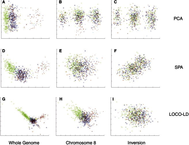
The Effect of a Long-Range LD Region Spanning an Inversion on Chromosome 8 on the Localization of a Spanish Data Set

The samples of the Spanish data set were localized with PCA, SPA, and LOCO-LD. The colors and marker types, defined in Figure 4, give the samples’ communities of origin.

(A, D, and G) The localization estimates (x versus y coordinates) of PCA (A), SPA (D), and LOCO-LD (G) on the entire Spanish data set.

(B, E, and H) The results of PCA (B), SPA (E), and LOCO-LD (H) when only chromosome 8 was used.

(C, F, and I) The results of PCA (C), SPA (F), and LOCO-LD (I) when only the inversion region was used.

In some cases, strong effects resulting from long inversions can be detected and manually removed from the analysis. We checked whether shorter inversions (or other regions of continuous high LD) could cause biases that would go undetected in the top PCs but still affect localization accuracy. We simulated this scenario by adding to each POPRES LD-pruned genotype the inversion genotype of a randomly drawn Spanish sample. In different experiments, we used either the whole inversion or shorter parts of it. We localized the samples by using SMARTPCA and SPA. The results are presented in Table 6 and show that already when the length of the added inversion was less than 25% of the original inversion, SMARTPCA showed a 12% increase in error. Overall, SPA was more robust than SMARTPCA to the inversion effect, and when the full inversion was introduced, the three-cluster pattern took over PCA’s map, whereas SPA’s error increased by only 14 km.

Table 6.

Comparison of the Effect of Long-Range LD Regions of Varying Lengths on SMARTPCA and SPA

Method	Inversion Length (SNPs)	Euclidean Distance: 2nd[1st, 3rd] Quartile	Distance: 2nd[1st, 3rd] Quartile (km)	Relative to Length 0
SMARTPCA pruned	0	2.78 [1.67, 4.61]	247.1 [155.0, 378.3]	1
SMARTPCA pruned	410	3.18 [1.84, 5.30]	275.7 [162.7, 433.4]	1.12
SMARTPCA pruned	1,800 (whole)	6.98 [4.18, 11.9]	545.4 [362.6, 832.9]	2.21
SPA pruned	0	2.55 [1.56, 4.02]	226.4 [137.7, 336.2]	1
SPA pruned	450	2.60 [1.58, 4.03]	227.3 [139.5, 336.8]	1.00
SPA pruned	900	2.63 [1.58, 4.09]	230.3 [139.4, 344.6]	1.02
SPA pruned	1,800 (whole)	2.73 [1.61, 4.23]	240.6 [141.8, 355.7]	1.06

The genotypes of the Spanish samples from the chromosome 8 inversion were excised, trimmed to different lengths, and “transplanted” in the genotypes of the POPRES samples. “Inversion length” gives the number of SNPs in the transplanted inversion out of the entire 1,800 SNPs in the inversion region. Reported error measures are the same as in Table 1. “Relative to Length 0” gives, per method, the ratio between the median error (in km) and the result before the inversion was added.

We went on to improve LOCO-LD’s localization analysis by setting a threshold on the maximum number of samples that were used from each community in each training session (n ≤ 50) and adjusting the window size to 10. Figure 4 depicts the inferred locations for communities in the northern part of Spain. The samples from each of the communities are well clustered together, except for a few outliers. The relative positions of these clusters partially reflect the true relations: the clusters of Galicia, Asturias, Castilla y León, Cantabria, and Aragón are correctly positioned, whereas Navarra, the País Vasco, and La Rioja are stretched to the northeast. The communities in the south of Spain do not cluster as clearly (see Figure S2), and samples from different communities tend to overlap, although the relative positions are conserved to a limited extent. The difference between the north and the south is probably at least partially attributed to the northern mountain chains, which separate the different communities. Such geographical barriers, which are absent from the south, decrease gene flow between the populations and extenuate the genetic differences between them.

Figure 4.

LOCO-LD’s Localization Results for Northern Spain

The figure depicts the inferred locations for individuals from different autonomous communities in the northern part of Spain. A description of the data set is given in Results section “Robustness to Long-Range LD: Results for a Spanish Data Set.” The number of training samples from each community is limited to 50. LOCO-LD’s version is genotypic with window length 10. The marker colors and types give the samples’ reported community of origin. The map at the top left depicts the true geographic locations of the communities. See Web Resources for background-image attribution.

Discussion

Existing methods for the geographic localization of genetic samples, including the commonly used PCA, do not account for LD between variants. In this paper, we have demonstrated that ignoring LD leads to a loss of accuracy when a commonly used SNP chip is used. Between-marker correlations impair the performance of the methods, and pruning the SNPs to obtain linkage equilibrium, as is often done with the use of PCA, entails discarding useful information. In addition, regions of long-range LD can dramatically bias the analysis results.

We have presented LOCO-LD, a localization method that incorporates an LD correction within an explicit probabilistic model. LOCO-LD successfully utilizes the information contained in variant sets of increasing density, making it the best-performing localization method among the methods we tested on the POPRES data set. This property should become critical as variant sets become increasingly large. Although examining the effect of accurate localization on downstream analysis is beyond the scope of this work, we note that accurate methods for geographic localization are already being used in the context of correction for population stratification in GWASs,²⁹ and LOCO-LD can be directly employed in such a framework. LOCO-LD also performs well when only a fraction of the genome is given, suggesting that it is appropriate for the analysis of genomic fragments extracted from admixed individuals in a framework previously proposed,¹⁵ as well as for integration within a local-ancestry-inference method similar to existing approaches.^16,30

Although we focused on continuous ancestry estimation in this work, much previous work has been performed in the context of discrete ancestry assignment. One of these works, by Lee et al.,³¹ deals with the problem of clustering genetic samples according to population of origin. The first stage of this method, which is based on a spectral-graph approach, includes a PCA modification that is meant to alleviate its sensitivity to outliers. In order to adjust the method to the localization task, we implemented the proposed kernel transformation stage for the LD-pruned POPRES genotype matrix and tested whether the eigenvectors of the resulting matrix can be used for localization. We found that the combination of the second and the third PCs yields accurate results (median error of 227 km). These results suggest that outlier regularization is an important factor in the localization of the POPRES data set and that the incorporation of such regularization into spatial modeling is likely to be beneficial. We note that we also experimented with extensions of additional ancestry-inference methods to the continuous localization scenario^32,33 but had limited success.

Although capturing certain properties of the genetic-flow process, the functions that link the geographic location to the allele frequencies in both SPA and LOCO-LD’s models remain restricted even when the addition of higher-order factors is allowed for. Introducing more flexibility into these functions is likely to provide a considerable improvement to these methods; specifically, model-based functions based on population-genetics theory might perform well, and we view this as a promising direction for further study.

Another area for further improvement would be a more principled adjustment of the window sizes according to the empirical LD patterns observed in the data in an attempt to increase the amount of LD captured while decreasing the noise. One could perform this by increasing the window size in regions where LD extends longer and setting the window boundaries according to LD hotspots.

Finally, we expect that allowing for position-dependent LD would constitute a major contribution to the spatial probabilistic approach. In addition to enabling more accurate modeling, the fact that LD patterns are likely to exhibit continuous change over space should allow their use as additional information for localization.

Appendix A: Closed-Form Optimization Formulas

Maximizing over β Given x

Given the genotypes of n individuals and their corresponding d × 1 position vectors x₁…x_n, we wish to obtain a maximum-likelihood estimator for β_j, the l × d coefficient matrix of window j of size l. If we denote the genotype segments included in window j as g_1j…g_nj, the per-window likelihood expression is

$$\mathcal{L}\left(g_{1j}\dots g_{nj};{\beta }_j,{\text{Σ}}_j\right)=\prod _{i=1}^n\frac{1}{{\left(2\pi \right)}^{\frac{l}{2}}{\left|{\text{Σ}}_j\right|}^{\frac{1}{2}}}{e}^{-\frac{1}{2}{\left({\beta }_j{x}_i-g_{ij}\right)}^T{\text{Σ}}_j^{-1}\left({\beta }_j{x}_i-g_{ij}\right)},$$ (Equation A1)

where Σ_j is the l × l matrix of pairwise correlations within the window.

We wish to obtain a maximum-likelihood estimator for β_j. Note that an equivalent expression to optimize is the total Mahalanobis distance,

$$f=\sum _{i=1}^n{\left({\beta }_j{x}_i-g_{ij}\right)}^T{\text{Σ}}_j^{-1}\left({\beta }_j{x}_i-g_{ij}\right).$$ (Equation A2)

Let G_j denote the l × n matrix, whose columns are the genotypes within window j of the samples with known origins, and let X denote the d × n matrix, whose columns are these origins. The derivative of the above formula as a function of β_j is

$$\begin{array}{c}\frac{\partial f}{\partial {\beta }_j}=\frac{\partial \sum _{i=1}^n{\left({\beta }_j{x}_i-g_{ij}\right)}^T{\text{Σ}}_j^{-1}\left({\beta }_j{x}_i-g_{ij}\right)}{\partial {\beta }_j}\\ =\sum _{i=1}^n\frac{\partial \left[x_i^T{\beta }_j^T{\text{Σ}}_j^{-1}{\beta }_j{x}_i-2g_{ij}^T{\text{Σ}}_j^{-1}{\beta }_j{x}_i\right]}{\partial {\beta }_j}\\ =\sum _{i=1}^n\left[2{\text{Σ}}_j^{-1}{\beta }_j{x}_i{x}_i^T-2\left({\text{Σ}}_j^{-1}{g}_{ij}{x}_i^T\right)\right]\\ =2{\text{Σ}}_j^{-1}{\beta }_j\left(\sum _{i=1}^n{x}_i{x}_i^T\right)-2{\text{Σ}}_j^{-1}\left(\sum _{i=1}^n{g}_{ij}{x}_i^T\right).\end{array}$$

By equating the derivative to 0, we obtain

$$\begin{array}{c}X{X}^T{\beta }_j^T=X{G}_j^T\\ \Rightarrow {\beta }_j^T={\left(X{X}^T\right)}^{-1}X{G}_j^T\\ \Rightarrow {\hat{\beta }}_j=G_j{X}^T{\left(X{X}^T\right)}^{-1}.\end{array}$$

Note that ${\hat{\beta }}_j$ is independent of Σ_j. Also note that the above result can be obtained per SNP and is not affected by the division to windows.

Maximizing over $\text{Σ}$ Given β and x

In order to obtain a maximum-likelihood estimator of Σ_j, we need to optimize the same likelihood as in Equation A1 but this time as a function of Σ_j. This is equivalent to the derivation of the maximum-likelihood estimator for the covariance matrix of a multivariate normal distribution, and the solution is

$${\hat{\Sigma }}_j=\frac{1}{n}\sum _{i=1}^n\left({\beta }_j{x}_i-g_{ij}\right){\left({\beta }_j{x}_i-g_{ij}\right)}^T.$$

The resulting matrix might not be full rank. If this is the case, we turn it into a full-rank matrix by adding $\lambda I_l$ for $0<\lambda \ll 1$; this is the same correction performed in Ridge regression.

Maximizing over x Given β and $\text{Σ}$

Given the parameters β_j and Σ_j for windows j = l…m and given the genotype of a new sample g₁…g_m, we wish to obtain an estimate for the new sample’s position vector x. The total Mahalanobis distance to be maximized as a function of x is

$$f=\sum _{j=1}^m{\left({\beta }_{j}x-g_j\right)}^T{\text{Σ}}_j^{-1}\left({\beta }_{j}x-g_j\right).$$ (Equation A3)

The position vector might include fixed values over which we do not wish to optimize; for example, we might decide to allow for an arbitrary offset in the genotype expectation by adding a third entry that is always set to 1 to the vector of geographical coordinates. We intend to optimize only over the nonfixed entries of x. Let $\dot{x}$ and $\ddot{x}$ denote the nonfixed and fixed parts of x, respectively, and let $\dot{\beta }$ and $\ddot{\beta }$ denote the corresponding parts of β. After the fixed genotype component $a_j={\ddot{\beta }}_j\ddot{x}$ is precomputed per window, the derivation becomes

$$\begin{array}{c}\frac{\partial f}{\partial x}=\frac{\partial \sum _{j=1}^m{\left({\dot{\beta }}_j\dot{x}+a_j-g_j\right)}^T{\text{Σ}}_j^{-1}\left({\dot{\beta }}_j\dot{x}+a_j-g_j\right)}{\partial \dot{x}}\\ =\frac{\partial \sum _{j=1}^m{\left({\dot{\beta }}_j\dot{x}-\left(g_j-a_j\right)\right)}^T{\text{Σ}}_j^{-1}\left({\dot{\beta }}_j\dot{x}-\left(g_j-a_j\right)\right)}{\partial \dot{x}}\\ =\frac{\partial \sum _{j=1}^m\left[{\dot{x}}^T{\dot{\beta }}_j^T{\text{Σ}}_j^{-1}{\dot{\beta }}_j\dot{x}-2{\left(g_j-a_j\right)}^T{\text{Σ}}_j^{-1}{\dot{\beta }}_j\dot{x}\right]}{\partial \dot{x}}\\ =\sum _{j=1}^m\left[2{\dot{\beta }}_j^T{\text{Σ}}_j^{-1}{\dot{\beta }}_j\dot{x}-2{\dot{\beta }}_j^T{\text{Σ}}_j^{-1}\left(g_j-a_j\right)\right]\\ =2\sum _{j=1}^m\left[{\dot{\beta }}_j^T{\text{Σ}}_j^{-1}{\dot{\beta }}_j\right]\dot{x}-2\sum _{j=1}^m\left[{\dot{\beta }}_j^T{\text{Σ}}_j^{-1}\left(g_j-a_j\right)\right]\\ \Rightarrow \hat{\dot{x}}={\left(\sum _{i=1}^m{\dot{\beta }}_j^T{\text{Σ}}_j^{-1}{\dot{\beta }}_j\right)}^{-1}\left(\sum _{i=1}^m{\dot{\beta }}_j^T{\text{Σ}}_j^{-1}\left(g_j-a_j\right)\right).\end{array}$$

Web Resources

The URLs for data presented herein are as follows:

• Background image in Figure 4, http://commons.wikimedia.org/wiki/File:Autonomous_communities_of_Spain.svg

• LOCO-LD, www.cs.tau.ac.il/∼heran/cozygene/software.shtml

References

- 1.Price A.L., Zaitlen N.A., Reich D., Patterson N. New approaches to population stratification in genome-wide association studies. Nat. Rev. Genet. 2010;11:459–463. doi: 10.1038/nrg2813. [DOI] [PMC free article] [PubMed] [Google Scholar]
- 2.Seldin M.F., Pasaniuc B., Price A.L. New approaches to disease mapping in admixed populations. Nat. Rev. Genet. 2011;12:523–528. doi: 10.1038/nrg3002. [DOI] [PMC free article] [PubMed] [Google Scholar]
- 3.Price A.L., Patterson N.J., Plenge R.M., Weinblatt M.E., Shadick N.A., Reich D. Principal components analysis corrects for stratification in genome-wide association studies. Nat. Genet. 2006;38:904–909. doi: 10.1038/ng1847. [DOI] [PubMed] [Google Scholar]
- 4.Jarvis J.P., Scheinfeldt L.B., Soi S., Lambert C., Omberg L., Ferwerda B., Froment A., Bodo J.M., Beggs W., Hoffman G. Patterns of ancestry, signatures of natural selection, and genetic association with stature in Western African pygmies. PLoS Genet. 2012;8:e1002641. doi: 10.1371/journal.pgen.1002641. [DOI] [PMC free article] [PubMed] [Google Scholar]
- 5.Bryc K., Velez C., Karafet T., Moreno-Estrada A., Reynolds A., Auton A., Hammer M., Bustamante C.D., Ostrer H. Colloquium paper: genome-wide patterns of population structure and admixture among Hispanic/Latino populations. Proc. Natl. Acad. Sci. USA. 2010;107(Suppl 2):8954–8961. doi: 10.1073/pnas.0914618107. [DOI] [PMC free article] [PubMed] [Google Scholar]
- 6.Hinch A.G., Tandon A., Patterson N., Song Y., Rohland N., Palmer C.D., Chen G.K., Wang K., Buxbaum S.G., Akylbekova E.L. The landscape of recombination in African Americans. Nature. 2011;476:170–175. doi: 10.1038/nature10336. [DOI] [PMC free article] [PubMed] [Google Scholar]
- 7.Wegmann D., Kessner D.E., Veeramah K.R., Mathias R.A., Nicolae D.L., Yanek L.R., Sun Y.V., Torgerson D.G., Rafaels N., Mosley T. Recombination rates in admixed individuals identified by ancestry-based inference. Nat. Genet. 2011;43:847–853. doi: 10.1038/ng.894. [DOI] [PMC free article] [PubMed] [Google Scholar]
- 8.Gravel S., Henn B.M., Gutenkunst R.N., Indap A.R., Marth G.T., Clark A.G., Yu F., Gibbs R.A., Bustamante C.D., 1000 Genomes Project Demographic history and rare allele sharing among human populations. Proc. Natl. Acad. Sci. USA. 2011;108:11983–11988. doi: 10.1073/pnas.1019276108. [DOI] [PMC free article] [PubMed] [Google Scholar]
- 9.Yang J.J., Cheng C., Devidas M., Cao X., Fan Y., Campana D., Yang W., Neale G., Cox N.J., Scheet P. Ancestry and pharmacogenomics of relapse in acute lymphoblastic leukemia. Nat. Genet. 2011;43:237–241. doi: 10.1038/ng.763. [DOI] [PMC free article] [PubMed] [Google Scholar]
- 10.Menozzi P., Piazza A., Cavalli-Sforza L. Synthetic maps of human gene frequencies in Europeans. Science. 1978;201:786–792. doi: 10.1126/science.356262. [DOI] [PubMed] [Google Scholar]
- 11.Yang W.Y., Novembre J., Eskin E., Halperin E. A model-based approach for analysis of spatial structure in genetic data. Nat. Genet. 2012;44:725–731. doi: 10.1038/ng.2285. [DOI] [PMC free article] [PubMed] [Google Scholar]
- 12.Price A.L., Weale M.E., Patterson N., Myers S.R., Need A.C., Shianna K.V., Ge D., Rotter J.I., Torres E., Taylor K.D. Long-range LD can confound genome scans in admixed populations. Am. J. Hum. Genet. 2008;83:132–135. doi: 10.1016/j.ajhg.2008.06.005. author reply 135–139. [DOI] [PMC free article] [PubMed] [Google Scholar]
- 13.Tian C., Plenge R.M., Ransom M., Lee A., Villoslada P., Selmi C., Klareskog L., Pulver A.E., Qi L., Gregersen P.K., Seldin M.F. Analysis and application of European genetic substructure using 300 K SNP information. PLoS Genet. 2008;4:e4. doi: 10.1371/journal.pgen.0040004. [DOI] [PMC free article] [PubMed] [Google Scholar]
- 14.Nelson M.R., Bryc K., King K.S., Indap A., Boyko A.R., Novembre J., Briley L.P., Maruyama Y., Waterworth D.M., Waeber G. The Population Reference Sample, POPRES: a resource for population, disease, and pharmacological genetics research. Am. J. Hum. Genet. 2008;83:347–358. doi: 10.1016/j.ajhg.2008.08.005. [DOI] [PMC free article] [PubMed] [Google Scholar]
- 15.Johnson N.A., Coram M.A., Shriver M.D., Romieu I., Barsh G.S., London S.J., Tang H. Ancestral components of admixed genomes in a Mexican cohort. PLoS Genet. 2011;7:e1002410. doi: 10.1371/journal.pgen.1002410. [DOI] [PMC free article] [PubMed] [Google Scholar]
- 16.Baran Y., Pasaniuc B., Sankararaman S., Torgerson D.G., Gignoux C., Eng C., Rodriguez-Cintron W., Chapela R., Ford J.G., Avila P.C. Fast and accurate inference of local ancestry in Latino populations. Bioinformatics. 2012;28:1359–1367. doi: 10.1093/bioinformatics/bts144. [DOI] [PMC free article] [PubMed] [Google Scholar]
- 17.Price A.L., Tandon A., Patterson N., Barnes K.C., Rafaels N., Ruczinski I., Beaty T.H., Mathias R., Reich D., Myers S. Sensitive detection of chromosomal segments of distinct ancestry in admixed populations. PLoS Genet. 2009;5:e1000519. doi: 10.1371/journal.pgen.1000519. [DOI] [PMC free article] [PubMed] [Google Scholar]
- 18.Wen X., Stephens M. Using linear predictors to impute allele frequencies from summary or pooled genotype data. Ann Appl Stat. 2010;4:1158–1182. doi: 10.1214/10-aoas338. [DOI] [PMC free article] [PubMed] [Google Scholar]
- 19.Menelaou A., Marchini J. Genotype calling and phasing using next-generation sequencing reads and a haplotype scaffold. Bioinformatics. 2013;29:84–91. doi: 10.1093/bioinformatics/bts632. [DOI] [PubMed] [Google Scholar]
- 20.Churchhouse C., Marchini J. Multiway admixture deconvolution using phased or unphased ancestral panels. Genet. Epidemiol. 2013;37:1–12. doi: 10.1002/gepi.21692. [DOI] [PubMed] [Google Scholar]
- 21.Novembre J., Johnson T., Bryc K., Kutalik Z., Boyko A.R., Auton A., Indap A., King K.S., Bergmann S., Nelson M.R. Genes mirror geography within Europe. Nature. 2008;456:98–101. doi: 10.1038/nature07331. [DOI] [PMC free article] [PubMed] [Google Scholar]
- 22.Wang C., Zöllner S., Rosenberg N.A. A quantitative comparison of the similarity between genes and geography in worldwide human populations. PLoS Genet. 2012;8:e1002886. doi: 10.1371/journal.pgen.1002886. [DOI] [PMC free article] [PubMed] [Google Scholar]
- 23.Patterson N., Price A.L., Reich D. Population structure and eigenanalysis. PLoS Genet. 2006;2:e190. doi: 10.1371/journal.pgen.0020190. [DOI] [PMC free article] [PubMed] [Google Scholar]
- 24.Browning S.R., Browning B.L. Rapid and accurate haplotype phasing and missing-data inference for whole-genome association studies by use of localized haplotype clustering. Am. J. Hum. Genet. 2007;81:1084–1097. doi: 10.1086/521987. [DOI] [PMC free article] [PubMed] [Google Scholar]
- 25.Purcell S., Neale B., Todd-Brown K., Thomas L., Ferreira M.A., Bender D., Maller J., Sklar P., de Bakker P.I., Daly M.J., Sham P.C. PLINK: a tool set for whole-genome association and population-based linkage analyses. Am. J. Hum. Genet. 2007;81:559–575. doi: 10.1086/519795. [DOI] [PMC free article] [PubMed] [Google Scholar]
- 26.Shumaker M.D., Bryan P. Computing under the open sky. Sky Telescope. 1984;68:158. [Google Scholar]
- 27.Sinnott R.W. Virtues of the haversine. Sky Telescope. 1984;68:159. [Google Scholar]
- 28.Pritchard J.K., Przeworski M. Linkage disequilibrium in humans: models and data. Am. J. Hum. Genet. 2001;69:1–14. doi: 10.1086/321275. [DOI] [PMC free article] [PubMed] [Google Scholar]
- 29.Sul J.H., Eskin E. Mixed models can correct for population structure for genomic regions under selection. Nat. Rev. Genet. 2013;14:300. doi: 10.1038/nrg2813-c1. [DOI] [PubMed] [Google Scholar]
- 30.Brisbin A., Bryc K., Byrnes J., Zakharia F., Omberg L., Degenhardt J., Reynolds A., Ostrer H., Mezey J.G., Bustamante C.D. PCAdmix: principal components-based assignment of ancestry along each chromosome in individuals with admixed ancestry from two or more populations. Hum. Biol. 2012;84:343–364. doi: 10.3378/027.084.0401. [DOI] [PMC free article] [PubMed] [Google Scholar]
- 31.Lee A.B., Luca D., Klei L., Devlin B., Roeder K. Discovering genetic ancestry using spectral graph theory. Genet. Epidemiol. 2010;34:51–59. doi: 10.1002/gepi.20434. [DOI] [PMC free article] [PubMed] [Google Scholar]
- 32.Engelhardt B.E., Stephens M. Analysis of population structure: a unifying framework and novel methods based on sparse factor analysis. PLoS Genet. 2010;6:e1001117. doi: 10.1371/journal.pgen.1001117. [DOI] [PMC free article] [PubMed] [Google Scholar]
- 33.Alexander D.H., Novembre J., Lange K. Fast model-based estimation of ancestry in unrelated individuals. Genome Res. 2009;19:1655–1664. doi: 10.1101/gr.094052.109. [DOI] [PMC free article] [PubMed] [Google Scholar]
Associated Data
This section collects any data citations, data availability statements, or supplementary materials included in this article.