Computational identification of functional introns: high positional conservation of introns that harbor RNA genes

Abstract

An appreciable fraction of introns is thought to have some function, but there is no obvious way to predict which specific intron is likely to be functional. We hypothesize that functional introns experience a different selection regime than non-functional ones and will therefore show distinct evolutionary histories. In particular, we expect functional introns to be more resistant to loss, and that this would be reflected in high conservation of their position with respect to the coding sequence. To test this hypothesis, we focused on introns whose function comes about from microRNAs and snoRNAs that are embedded within their sequence. We built a data set of orthologous genes across 28 eukaryotic species, reconstructed the evolutionary histories of their introns and compared functional introns with the rest of the introns. We found that, indeed, the position of microRNA- and snoRNA-bearing introns is significantly more conserved. In addition, we found that both families of RNA genes settled within introns early during metazoan evolution. We identified several easily computable intronic properties that can be used to detect functional introns in general, thereby suggesting a new strategy to pinpoint non-coding cellular functions.

INTRODUCTION

Spliceosomal introns are one of the defining features of eukaryotes and are found in virtually all fully sequenced eukaryotic genome. Generally, their sequence evolutionary rate resembles that of synonymous sites in coding regions, a fact that was widely interpreted as indicative of neutral evolution (1,2). In contrast, it was noticed that the position of introns along the coding region, i.e. their point of insertion with respect to the coding nucleotides, is remarkably conserved (3,4). How can this intron positional conservation (IPC) be settled with their apparent lack of sequence conservation?

In the past few decades, numerous demonstrations of intron functions have been reported, showing that many introns play critical roles in cellular regulatory programs (5). Consistent with the lack of sequence conservation, these functions are either sequence-independent or are carried out by short cis elements that contribute only little to the overall sequence conservation of the intron.

Applying birth–death models to intron position data, a picture of intron–exon evolution in eukaryotes had emerged (6,7). These studies showed that different eukaryotic clades are characterized by different rates of intron gain and loss, and they uncovered general evolutionary patterns such as massive intron gain during the genesis of early eukaryotic lineages, followed by predominance of intron loss events later on.

These reconstructions use data of many introns and therefore represent the evolutionary behavior of a ‘typical’, presumably non-functional, intron. We assert that a functional intron would experience a different selection regime, and therefore its evolutionary behavior will show unique features. Specifically, we hypothesize that functional introns will be more resistant to loss, thus showing higher positional conservation.

To test this, we examined the evolutionary history of a particular group of introns that are known to be functional by means of harboring RNA genes. Specifically, we looked at introns that harbor microRNAs (miRNAs) and snoRNAs. These introns are presumed to have a reduced loss rate, as their loss would result in the loss of their RNA content. Indeed, using multiple criteria for IPC, we found that RNA gene-bearing introns are more conserved, and that their evolutionary patterns are more remote from those of ‘typical’ introns. Moreover, we found that introns that harbor RNA genes show signs of elevated positional conservation mainly within the metazoan clade, suggesting that the association between RNA genes and introns dates back to the very early days of the metazoan lineage.

MATERIALS AND METHODS

Gene architecture data set

We have generated an intron–exon data set comprising the full genomes of 98 eukaryotic species, based on annotations from Ensembl release 61 (8) and Ensembl Genomes (9) via the BioMart interface (10), Refseq (11), UCSC genome browser (12), JGI (13), FlyBase (14), VectorBse (15), AphidBase (16), BeetleBase (17), SilkDB (18), Fourmidable (19) and the Hymenoptera Genome Database (20) (Supplementary Table S1).

Orthology assignment

In the current study, we focus on introns that harbor miRNAs or snoRNAs. Based on miRBase (21) and sno/scaRNAbase (22), we mapped the position of these RNA genes onto our annotated genomes and identified all miRNA/snoRNA-bearing introns. In human, such introns were found in 450 genes. These RNA genes are best annotated in human, and we have therefore used these 450 genes as the basis for subsequent analysis.

For these 450 genes, we queried the Ensembl Compara database (23) via their Perl API to detect orthologs in our 98 species. Frequently, a set of orthologous genes contained multiple subsets of paralogs. In such cases, we wished to identify the single best representative from each species. This was done by calculating, within each set of orthologs, the sum of pairwise distances of all possible gene combinations that contain exactly one ortholog per species. The representative set was chosen to be the one with the minimal sum of pairwise distances.

The resulting 450 sets of orthologous genes were partial in the sense that most of them contained orthologs for far less than 98 species. To this end, species with an ortholog in <85% of the sets were removed from the data set, unless they were the only representative of their respective taxonomic group. In taxonomic groups with high sampling (e.g. mammals), we left for analysis the species with the largest number of orthologs. This process left 391 sets of orthologs over 28 species (Supplementary Table S2): one insect (Drosophila melanogaster), one bird (Gallus gallus), two fish (Danio rerio, Gasterosteus aculeatus), two amphibians (Anolis carolinensis, Xenopus tropicalis), three invertebrates (Caenorhabditis elegans, Schistosoma mansoni, Ciona savignyi), four fungi (Ustilago maydis, Saccharomyces cerevisiae, Neurospora crassa, Schizosaccharomyces pombe), four plants (Vitis vinifera, Arabidopsis thaliana, Physcomitrella patens, Oryza sativa), five protists (Plasmodium falciparum, Dictyostelium discoideum, Leishmania major, Phaeodactylum tricornutum, Phytophthora infestans) and six mammals (Homo sapiens, Pan troglodytes, Mus musculus, Pongo abelii, Ornithorhynchus anatinus, Monodelphis domestica). Notably, many sets of orthologs are still missing representative from some species, and these were regarded as missing data.

Phylogenetic tree

The phylogenetic tree for the 28 species was formed by combining taxonomic data from The Tree of Life Web Project (http://tolweb.org/), NCBI (24,25) and FlyBase (14). Divergence times were estimated based on Time Tree (26). iTOL (27) was used for tree display and modification (Supplementary Figure S1). When there were no data on the divergence time between two species, we used sequences with orthologs in close species with known divergence time to reconstruct the phylogeny using UPGMA (28). Then, we estimated the missing divergence times by linear regression. As future analysis steps require a bifurcating tree, multifurcations were resolved by a series of bifurcations, separated by short (100 000 years) internal branches.

Multiple alignments

We used MUSCLE (29) to align the protein products of the transcripts within each set of orthologs, then applied the Matlab function seqinsertgaps to get the multiple alignment at the mRNA level.

Intron presence/absence patterns

Upon each multiple sequence alignment, we projected the positions of the exon–exon junctions and transferred the alignment into ternary representation where 1 stands for the last nucleotide of an exon, 0 stands for all other nucleotides and 2 stands for gaps and other missing data. For example, a species that lacks an ortholog in one of the sets will have an entire row of 2’s in the multiple alignment. A multiple alignment of positions over species will be represented by a ternary matrix of size . Each column in this matrix is called a pattern, and it represents the intron phylogenetic presence–absence pattern in a particular position along the coding region (Figure 1a and b). Overall, our data consist of 1 474 563 patterns, which is just the number of positions in the collection of the 391 multiple alignments. In the following analysis, we assume that each position evolves independently of other positions, allowing us to represent the data more succinctly by the list of all 29 516 unique patterns, along with the number of times each unique pattern appears in the data (Figure 1c). Hereinafter, we shall denote by the number of occurrences of unique pattern .

Figure 1.

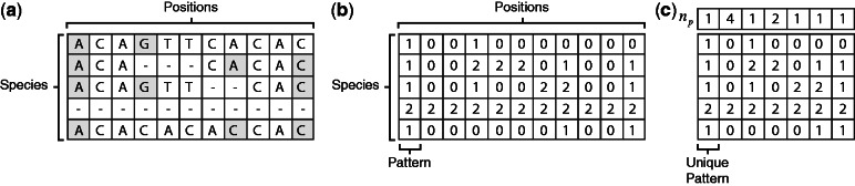
Ternary representation of multiple alignments. (a) A toy example of a multiple sequence alignment of an orthologous group. The rows stand for species, and the columns represent the position along the alignment. The last nucleotide of an exon is highlighted. (b) A ternary representation of the same alignment: 1 stands for the last nucleotide of an exon, 0 stands for all other nucleotides and 2 stands for gaps or missing orthologs. (c) The same data are represented by a list of unique patterns, and by the number of times each of them appears in the data ().

We filtered out patterns consisting ≥45% unknowns (2’s), as statistical inference from these would be less reliable. Patterns without a 1 were filtered out as well, as they do not contain information on intron positions. Also, as we base the analysis on human RNA gene-bearing introns, we filtered out patterns with 2’s in human. These steps reduced the number of unique patterns from 29 516 to 4163.

miRNA/snoRNA-bearing patterns

A pattern is called miRNA-bearing pattern if it designates the presence of an intron in human (a ‘1’ in the human row), and if that intron harbors a miRNA. If in all appearances of unique pattern , it is miRNA-bearing, then the unique pattern is called miRNA-bearing unique pattern. If in some appearances, it is miRNA-bearing and in others it is not, it is called miRNA-mixed unique pattern. Otherwise, it is called miRNA-lacking unique pattern (Figure 2). In a similar fashion, we define snoRNA-bearing unique patterns, snoRNA-lacking unique patterns and snoRNA-mixed unique patterns.

Figure 2.

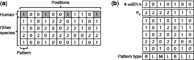
Types of unique patterns. (a) A ternary representation of a multiple sequence alignment. Human introns—depicted as 1 in the first row—that bear miRNAs are highlighted. (b) The same data are represented by a list of unique patterns, by the number of times each of them appears in the data (), and by the number of times each pattern contains miRNAs in the human intron. The last row specifies the pattern type: ‘B’ for miRNA-bearing, ‘L’ for miRNA-lacking and ‘M’ for miRNA-mixed.

Overall, our data consist of 53 miRNA-bearing, 4099 miRNA-lacking, 11 miRNA-mixed, 99 snoRNA-bearing, 4041 snoRNA-lacking and 23 snoRNA-mixed unique patterns (Supplementary Figure S2). Clearly, hosting miRNAs and snoRNAs are not mutually exclusive, and three unique patterns are both miRNA-bearing and snoRNA-bearing (Supplementary Table S3).

Reconstruction of gene architecture evolution

In past works, we have devised a comprehensive model of gene architecture evolution (4). This model is implemented in the Evolutionary Reconstruction by Expectation-Maximization (EREM) software tool (http://carmelab.huji.ac.il/software.html#erem) that learns the model parameters and reconstructs the evolutionary history of the intron–exon structure. EREM allows for gene-, site- and tree-branch variability in intron loss and gain rates, as well as an ability to handle missing data in the input (2’s in the aforementioned alignment matrices). EREM’s input is the ternary patterns and the known phylogenetic tree, and its output is the estimated model parameters and the probability of having an intron in each position for any of the internal nodes in the tree.

A pattern is defined over the leaves of the tree (terminal nodes), and its likelihood is the probability of observing it, given the model parameters, see formula 15 in Carmel et al. (4). For each unique pattern , we use either Dollo parsimony or EREM to find the last common ancestor (LCA) of the intron in all intron-bearing terminal nodes. Hereinafter, we shall assume that the intron originated (was gained) along the lineage leading to LCA.

Pattern features

To find whether miRNA/snoRNA-bearing patterns have unique properties, we compiled a list of 48 pattern-characterizing features (Supplementary Table S4). Features that are highly associated with another feature (absolute value of the correlation coefficient above 0.85) were removed, leaving a final list of 13 features (Table 1). These 13 features describe various properties of the patterns, including their level of positional conservation, how typical they are when compared with the evolutionary pattern of ‘typical’ introns, how ancient the intron is and where along the coding sequence (CDS) the intron is present (Supplementary Table S4).

Table 1.

The final set of 13 pattern-characterizing features used in the analysis

Feature	Description
LOGLIKE	Given EREM’s estimation of the evolutionary model parameters, this is the log-likelihood of observing the pattern.
ONES_RATIO_KNOWN	The number of 1’s divided by the total number of 1’s and 0’s in the pattern.
SANKOFF_G3L1	The minimum number of intron gain and loss events required to obtain the pattern, given that gains cost three times as much as losses (using the Sankoff algorithm).
SANKOFF_G1L3	The minimum number of intron gain and loss events required to obtain the pattern, given that losses cost three times as much as gains (using the Sankoff algorithm).
IN_AMPHIBIAN	This feature is 1 if the pattern has a 1 in at least one amphibian (A. carolinensis or X. tropicalis), otherwise it is 0.
IN_FISH	This feature is 1 if the pattern has a 1 in at least one fish (D. rerio or G. aculeatus), otherwise it is 0.
IN_BIRD	This feature is 1 if the pattern has a 1 in G. gallus otherwise it is 0.
IN_FUNGI	This feature is 1 if the pattern has a 1 in at least one fungi (U. maydis, S. pombe, S. cerevisiae or N. crassa), otherwise it is 0.
IN_PLANT	This feature is 1 if the pattern has a 1 in at least one plant (V. vinifera, A. thaliana, P. patens or O. sativa), otherwise it is 0.
IN_PROTIST	This feature is 1 if the pattern has a 1 in at least one protist (P. falciparum, D. discoideum, L. major, P. tricornutum or P. infestans), otherwise it is 0.
LCA_AGE	The LCA of all the intron-bearing species is assumed to be the species in which the intron was originated. LCA_AGE is the age of LCA [MYA].
MED_REL_POSITION	The median distance of the exon–exon junction from the beginning of the CDS divided by the CDS length.
MED_POSITION	The median distance of the exon–exon junction from the beginning of the CDS (nucleotides).

Statistical tests

We tested whether miRNA/snoRNA-bearing unique patterns have distinct characteristic values of each feature using the Mann–Whitney U-test and t-test with unknown and equal variance (30).

Fisher discriminant analysis

Fisher discriminant analysis is a supervised linear dimensionality reduction technique that projects the data into a low-dimensional space such that clusters are best separated (31). Here, we used the Fisher discriminant analysis to separate miRNA/snoRNA-bearing unique patterns from miRNA/snoRNA-lacking unique patterns. Interpreting the composition of the Fisher discriminant vector requires caution, as it is implied that the features are independent. In our analysis, this is not the case. To overcome this, we first applied principal component analysis to the data and then used the Fisher discriminant analysis on the projection of the data onto the space spanned by the first seven principal components (which are, of course, assured to be independent).

RESULTS AND DISCUSSION

Gene architecture data

We identified 450 human genes whose introns harbor miRNAs or snoRNAs. Of those, for 391 genes, we were able to identify sufficient number of orthologs from among 27 other eukaryotic species (see ‘Materials and Methods’ section). For each of the 391 orthologous groups, we computed the multiple alignment of the proteins and represented it by a ternary matrix at the underlying mRNA level, denoting by 1, the last nucleotide of an exon; by 0, any other nucleotide; and by 2, any missing value such as gap or lack of ortholog (Figure 1a and b; see more details in ‘Materials and Methods’ section). Each column (position) in this matrix is denoted a pattern. A ‘1’ in a pattern stands for an exon–exon junction in the mRNA of the corresponding species, and thus a pattern reflects the intron presence/absence distribution across species at a specific position. The entire data set consists of 1 474 563 patterns (positions), but filtering out patterns that are not relevant to the current study (see ‘Materials and Methods’ section) left a final set of 169 genes and a total of 5653 patterns. The same pattern may appear multiple times in the alignments, and we have thus summarized the data by compiling a list of all 4163 unique patterns and by denoting by the number of occurrences of unique pattern (Figure 1c).

We have put together a list of 48 pattern-characterizing features (Supplementary Table S4), and after filtering out features that are highly dependent on others, we were left with a final set of 13 features (see ‘Materials and Methods’ section; Table 1). These features are associated with the level of IPC, with how typical the pattern is, with how ancient the intron is and with where along the CDS the RNA gene-bearing intron resides.

MiRNA-bearing patterns have unique characteristics

The 169 genes contain 64 human intronic miRNAs. We have referred to the pattern corresponding to a miRNA-bearing human intron (the pattern for the last nucleotide of the upstream exon) as a miRNA-bearing pattern. We divided the unique patterns into three groups: an miRNA-bearing unique pattern is a unique pattern with a miRNA-bearing human intron in all occurrences; an miRNA-mixed unique pattern is a unique pattern with a human intron that bears miRNA in some occurrences, and lacks miRNA in others; otherwise, a unique pattern will be denoted miRNA-lacking unique pattern (Figure 2). Overall, the data comprise 53 miRNA-bearing, 4099 miRNA-lacking and 11 miRNA-mixed unique patterns (Supplementary Figure S2a).

To see what features characterize miRNA-bearing unique patterns, we tested each feature for whether it differs significantly between miRNA-bearing and miRNA-lacking unique patterns (using Bonferroni-corrected t-test; Table 2). Ten of the thirteen features were found to be significantly different in miRNA-bearing unique patterns, suggesting that these patterns have special attributes that will be discussed in the next sections. We repeated the analysis using the Mann–Whitney U-test and obtained identical conclusions (Table 2).

Table 2.

Mean and median of the 13 features for miRNA-bearing and miRNA-lacking unique patterns

Feature	Mean			Median
	miRNA-bearing pattern	miRNA-lacking pattern	P-value (t-test)	miRNA-bearing pattern	miRNA-lacking pattern	P-value (U-test)
LOGLIKE	−17.99	−13.63	7.1·(10−4)	−15.52	−11.62	5.3·(10−6)
ONES_RATIO_KNOWN	0.52	0.22	9.6·(10−21)	0.50	0.06	1.1·(10−15)
SANKOFF_G3L1	4.13	3.37	9.3·(10−5)	4	3	4.4·(10−5)
SANKOFF_G1L3	2.55	1.58	1.4·(10−7)	2	1	8.8·(10−9)
IN_AMPHIBIAN	0.96	0.62	4.1·(10−6)	1	1	4.3·(10−6)
IN_FISH	0.98	0.61	4.3·(10−7)	1	1	4.6·(10−7)
IN_BIRD	0.98	0.45	7.4·(10−14)	1	0	9.1·(10−14)
IN_FUNGI	0.62	0.59	1	1	1	1
IN_PLANT	0.96	0.72	1.4·(10−3)	1	1	1.4·(10−3)
IN_PROTIST	0.92	0.82	0.74	1	1	0.74
LCA_AGE	1104	460	2.2·(10−10)	993.6	0	1.7·(10−14)
MED_REL_POSITION	0.45	0.49	1	0.46	0.49	1
MED_POSITION	773.1	1461.5	1.2·(10−2)	426	982	6·(10−3)

P-values are Bonferroni corrected.

To test which linear combination of the features best characterizes miRNA-bearing unique patterns, we applied the Fisher linear discriminant analysis (see ‘Materials and Methods’ section). MiRNA-bearing unique patterns are distinguished by having high value of the Fisher discriminant vector and so are the miRNA-mixed unique patterns (Figure 3a). In fact, more than two-thirds of the miRNA-lacking unique patterns have their Fisher discriminant coordinate lower than that of any of the miRNA-bearing or miRNA-mixed unique patterns. The contribution of each feature to the Fisher discriminant vector is shown in Figure 3b (usually called a loading plot). As miRNA-bearing patterns have high positive values of the Fisher discriminant vector, they are characterized by high values of features with positive contribution and low values of features with negative contribution. The makeup of the Fisher discriminant vector is perfectly consistent with the tests on the individual features (Table 2), having negative contribution of LOGLIKE, MED_REL_POSITION and MED_POSITION, and positive contribution of all other features. These results suggest that human introns that harbor miRNAs show distinct properties, which we will discuss in the sections below.

Figure 3.

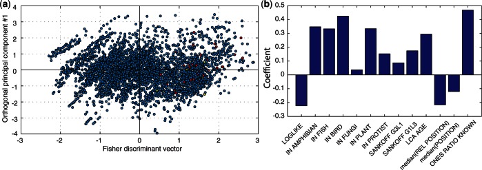
Fisher discriminant analysis for miRNA-bearing versus miRNA-lacking unique patterns. (a) Scatter plot of all unique patterns: (red) miRNA-bearing, (yellow) miRNA-mixed and (blue) miRNA-lacking unique patterns. The x-axis is the Fisher discriminant vector, and the y-axis was computed—for visualization only—as the first principal component that is constrained to be orthogonal to the Fisher discriminant vector. (b) The contribution of each of the 13 features to the Fisher discriminant vector. The y-axis is the coefficient of the respective feature in the linear combination that makes up the Fisher discriminant vector.

MiRNA-bearing patterns tend to be more conserved

Despite being characterized by more intron gain and loss events (SNAKOFF_G3L1 and SANKOFF_G1L3 in Table 2), probably owing to their antiquity (see next section), all conservation-related features suggest that miRNA-bearing introns have high positional conservation.

First, the log-likelihood of miRNA-bearing unique patterns (LOGLIKE) tends to be small, supporting the assumption that their evolutionary patterns are atypical when compared with the bulk of non-functional introns (Figure 4a). The average log-likelihood of miRNA-bearing unique patterns is −17.99, whereas it is −13.63 for miRNA-lacking unique patterns (P = 7.1·10⁻⁴, t-test; Table 2). This is consistent with a negative contribution of LOGLIKE to the Fisher discriminant vector (Figure 3b).

Figure 4.

Ranking of unique patterns. (Top rows) snoRNA-bearing (blue), snoRNA-mixed (red) and snoRNA-lacking (beige) unique patterns. (Bottom rows) miRNA-bearing (blue), miRNA-mixed (red) and miRNA-lacking (beige) unique patterns. The unique patterns are ranked according to (a) their log-likelihood; (b) the antiquity of the intron; and (c) their distance from CDS start.

Second, miRNA-bearing unique patterns are associated with introns that appear in human and, at exactly the same position, in other metazoans (IN_AMPHIBIAN, IN_FISH, IN_BIRD). This suggests that miRNA-bearing introns have a reduced loss rate in metazoans compared with miRNA-lacking introns. These introns show no tendency for positional conservation in fungi or various stem protists (IN_FUNGI, IN_PROTIST), suggesting that many of them have gained their miRNA content in early metazoans. Interestingly, when comparing the positional conservation of miRNA-bearing introns in human and plants, weak but significant conservation is detected (P = 0.0014, t-test; Table 2), consistent with other evidence for high positional conservation of introns between metazoans and plants (4,7).

Third, the feature that is most discriminating miRNA-bearing introns from miRNA-lacking ones is ONES_RATIO_KNOWN (Table 2 and Figure 3b), measuring the ratio of the number of introns present in that position (the number of 1’s in the pattern) to the total number of orthologous positions in our data set (the number of 0’s and 1’s in the pattern). A value of 1 means that all orthologs in which the position is present harbor an intron in that position. MiRNA-bearing introns show high values of ONES_RATIO_KNOWN, suggesting, again, that these introns have high positional conservation. The mean value of ONES_RATIO_KNOWN in miRNA-bearing unique patterns is 0.47, compared with only 0.22 for miRNA-lacking unique patterns (P = 9.6·10⁻²¹, t-test; Table 2).

In general, miRNAs are found in metazoans, plants and a variety of unicellular eukaryotes (32–34). Yet, as of today, proper miRNAs were not identified in fungi, although miRNA-like molecules had been found (35,36). Adding this to the fact that miRNA structure, function and biogenesis somewhat differ between metazoans and plants led to the notion that miRNAs entered independently to various eukaryotic clades (37). Our results show that the position of miRNA-bearing introns is extraordinarily conserved, but only within metazoans, rendering further credence to the view that miRNAs developed independently in metazoans.

miRNA-bearing introns tend to be ancient

For a given pattern, we assume that the intron was originally gained along the branch leading to the LCA of all species that harbor an intron at this position. The feature LCA_AGE measures the evolutionary age of this LCA and is therefore a proxy to how old the intron is. LCA_AGE contributes positively to the Fisher discriminant vector (Figure 3b), and, consistently, miRNA-bearing introns seem to have been gained early during eukaryotes evolution (Figure 4b). The mean LCA_AGE of miRNA-bearing unique patterns is 1104 million years ago (MYA), whereas it is only 460 MYA for miRNA-lacking unique patterns (P = 2.2·10⁻¹⁰, t-test; Table 2). This corroborates nicely with the finding of the previous section that miRNAs got inserted into introns in early metazoans, as the introns that were present then were necessarily of ancient origin. The EREM algorithm calculates the posterior probability of the presence of an intron at each ancestral node. As such, it can produce a different estimation of the intron origin than Dollo. We repeated the analysis with LCA_AGE calculated by EREM and received qualitatively same results (Supplementary Table S5).

Long first introns explain the tendency of miRNA-bearing introns to reside towards the 5′-end of the gene

The feature MED_POSITION is the median distance (in nucleotides) of the exon–exon junction from the beginning of the CDS in human, taken over all occurrences of the miRNA-bearing unique pattern. The feature MED_REL_POSITION is similar, except that the distance is divided by the CDS length. Both features show somewhat lower values for miRNA-bearing unique patterns (Table 2, Figure 3b), although, admittedly, this trend is weak (Figure 4c).

These results confirm a study by Zhou et al., (38) in which it was reported that miRNA-bearing introns tend to reside near the 5′-end of the gene. In this work, Zhou et al. also found that miRNAs tend to reside within long introns, but did not check the deep connection between the two observations. We hypothesized that neither trend is significant, and that these two observations can be explained by the well-known tendency of 5′-most introns (first introns) to be significantly longer (39). To test this, we assumed that an miRNA has an equal probability to get inserted at any position along the intron, regardless of its distance from the beginning of the CDS. Consequently, we ran 1000 simulations, in which we uniformly re-positioned miRNAs within the introns of their host genes. In >95% of the cases, a randomly positioned miRNA was located within its true host intron, or in another intron that is closer to the 5′-end of the gene. This shows that the observed tendency of miRNAs to reside towards the 5′-end of the gene is due to the unusual length of first introns. Notably, this observation does not necessarily rule out the possibility that natural selection does act to position RNA genes near the 5′ untranslated region (5′UTR), allowing them to be expressed early during transcription.

The unique characteristics of snoRNA-bearing patterns

We have mapped known snoRNAs into the human introns in our data set and found a total of 123 snoRNA-bearing introns. Similarly to the process with miRNAs, we divided the 4163 unique patterns into snoRNA-bearing unique patterns (99 patterns), snoRNA-mixed unique patterns (23 patterns) and snoRNA-lacking unique patterns (4041 patterns; Supplementary Figure S2b). We do not see any tendency of miRNAs and snoRNAs to reside within the same intron, as only three unique patterns are both miRNA-bearing and snoRNA-bearing (Supplementary Table S3).

Except for MED_REL_POSITION, all features significantly differ between snoRNA-bearing and snoRNA-lacking unique patterns (Table 3), suggesting that the two groups are characterized by a different set of features. Fisher discriminant analysis visually demonstrates this, as snoRNA-bearing and snoRNA-mixed unique patterns have high values of the Fisher discriminant vector (Figure 5a). The makeup of the Fisher discriminant vector is in complete agreement with Table 3 (Figure 5b).

Table 3.

Mean and median of the 13 features for snoRNA-bearing and snoRNA-lacking unique patterns

Feature	Mean			Median
	snoRNA-bearing pattern	snoRNA-lacking pattern	P-value (t-test)	snoRNA-bearing pattern	snoRNA-lacking pattern	P-value (U-test)
LOGLIKE	−22.49	−13.45	3.1·(10−29)	−18.58	−11.54	1.1·(10−19
ONES_RATIO_KNOWN	0.47	0.22	2.9·(10−28)	0.46	0.06	3.1·(10−23)
SANKOFF G3L1	4.79	3.34	4.8·(10−30)	5	3	5.3·(10−29)
SANKOFF G1L3	3.19	1.56	1.9·(10−39)	3	1	3.1·(10−34)
IN AMPHIBIAN	0.99	0.61	2.9·(10−13)	1	1	3.5·(10−13)
IN FISH	0.98	0.60	4·(10−13)	1	1	4.8·(10−13)
IN BIRD	0.95	0.44	4.1·(10−23)	1	0	7.6·(10−23)
IN FUNGI	0.41	0.60	3.3·(10−3)	0	1	3.3·(10−3)
IN PLANT	0.29	0.74	2.5·(10−22)	0	1	4.4·(10−22)
IN PROTIST	0.49	0.84	6.9·(10−18)	0	1	9.9·(10−18)
LCA AGE	1202.7	449	8.6·(10−26)	993.6	0	4.3·(10−31)
MED_REL_POSITION	0.51	0.49	1	0.52	0.49	1
MED_POSITION	740.7	1473	2.2·(10−5)	514	999	4.6·(10−7)

P-values are Bonferroni corrected.

Figure 5.

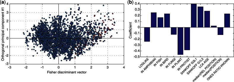
Fisher discriminant analysis for snoRNA-bearing versus snoRNA-lacking unique patterns. (a) Scatter plot of all unique patterns: (red) snoRNA-bearing, (yellow) snoRNA-mixed and (blue) snoRNA-lacking unique patterns. The x-axis is the Fisher discriminant vector, and the y-axis was computed—for visualization only—as the first principal component that is constrained to be orthogonal to the Fisher discriminant vector. (b) The contribution of each of the 13 features to the Fisher discriminant vector. The y-axis is the coefficient of the respective feature in the linear combination that makes up the Fisher discriminant vector.

Like in miRNA-bearing unique patterns, the features that characterize snoRNA-bearing unique patterns suggest that snoRNAs were inserted into introns in early metazoans, thereby conferring them with function and with increased resistance to loss. The log-likelihood of snoRNA-bearing unique patterns is substantially reduced (Figure 4a), with a mean of −22.49 compared with −13.45 in snoRNA-lacking unique patterns (P = 3.1·10⁻²⁹, t-test; Table 3). The features ONES_RATIO_KNOWN, IN_AMPHIBIAN, IN_FISH and IN_BIRD are all higher in snoRNA-bearing unique patterns, whereas IN_FUNGI, IN_PLANT and IN_PROTIST are lower (Table 3), again signifying early metazoan evolution as the point in time in which snoRNAs were attached to introns. This is further supported by higher values of LCA_AGE for snoRNA-bearing unique patterns (Figure 4b).

SnoRNAs are ancient RNA genes, fundamental to rRNA modifications in both archaea and eukaryotes (40). Yet, in different clades, they show very different genomic organization, ranging from independently transcribed units harboring their own promoter to intron-residing units whose transcription depends on that of the hosting gene. Comparative study of these genomic organizations showed that intron-residing snoRNAs are particularly abundant in metazoans, much less so in plants, and are almost absent in fungi (41). This finding is in perfect agreement with our conclusion that snoRNAs settled within introns in early metazoans.

CONCLUSIONS

In this work, we have focused on introns that are functional owing to RNA genes that they host. We found that such introns show distinct patterns of evolution, notably, a decreased loss rate since the time of function gain. In fact, we analyzed miRNA-bearing introns and snoRNA-bearing introns separately, and in both cases, we found that the functional introns have very similar characteristics (compare, e.g. Figures 3b and 5b). This leads us to hypothesize that elevated positional conservation is a property of functional introns in general, and not only of the specific family of introns that we have investigated. We therefore predict that a high fraction of the introns associated with high values of the Fisher discriminant vector (see Figures 3a and 5a) are functional, even if this function is not hosting RNA genes.

Finding functional non-coding elements like RNA genes, transcription factor binding sites and splicing factor binding sites are known to be much harder than finding protein-coding genes. Many factors contribute to this evasive nature of functional non-coding elements, such as short and degenerate sequence, poor sequence conservation and broad flexibility in genomic location. This work provides means to detect such otherwise invisible elements, at least when they reside within introns. Even more, some intronic functions do not depend on sequence at all but merely on the fact that splicing took place. This is, for example, how introns contribute to nuclear export (42) or to nonsense-mediated decay in mammals (43). As of today, such intronic functions withstand any computational prediction. Detection of introns with high positional conservation is therefore a novel, and actually the single, approach for computational identification of such functional introns. In this regard, intron position is a criterion by which evolutionary conservation can be measured, similarly to the more familiar criteria of sequence or structure conservation.

SUPPLEMENTARY DATA

Supplementary Data are available at NAR Online: Supplementary Tables 1–5 and Supplementary Figures 1 and 2.

FUNDING

European Union Marie Curie Reintegration Grant [IRG-248639]. Funding for open access charge: European Union Marie Curie Reintegration Grant [IRG-248639].

Conflict of interest statement. None declared.

REFERENCES

- 1.Hughes AL, Yeager M. Comparative evolutionary rates of introns and exons in murine rodents. J. Mol. Evol. 1997;45:125–130. doi: 10.1007/pl00006211. [DOI] [PubMed] [Google Scholar]
- 2.Graur D, Li WH. Fundamentals of Molecular Evolution. 2nd edn. Sunderland, MA, USA: Sinauer Associates; 2000. [Google Scholar]
- 3.Rogozin IB, Wolf YI, Sorokin AV, Mirkin BG, Koonin EV. Remarkable interkingdom conservation of intron positions and massive, lineage-specific intron loss and gain in eukaryotic evolution. Curr. Biol. 2003;13:1512–1517. doi: 10.1016/s0960-9822(03)00558-x. [DOI] [PubMed] [Google Scholar]
- 4.Carmel L, Rogozin IB, Wolf YI, Koonin EV. Patterns of intron gain and conservation in eukaryotic genes. BMC Evol. Biol. 2007;7:192. doi: 10.1186/1471-2148-7-192. [DOI] [PMC free article] [PubMed] [Google Scholar]
- 5.Chorev M, Carmel L. The function of introns. Front. Genet. 2012;3:55. doi: 10.3389/fgene.2012.00055. [DOI] [PMC free article] [PubMed] [Google Scholar]
- 6.Csuros M, Rogozin IB, Koonin EV. A detailed history of intron-rich eukaryotic ancestors inferred from a global survey of 100 complete genomes. PLoS Comput. Biol. 2011;7:e1002150. doi: 10.1371/journal.pcbi.1002150. [DOI] [PMC free article] [PubMed] [Google Scholar]
- 7.Carmel L, Wolf YI, Rogozin IB, Koonin EV. Three distinct modes of intron dynamics in the evolution of eukaryotes. Genome Res. 2007;17:1034–1044. doi: 10.1101/gr.6438607. [DOI] [PMC free article] [PubMed] [Google Scholar]
- 8.Flicek P, Amode MR, Barrell D, Beal K, Brent S, Carvalho-Silva D, Clapham P, Coates G, Fairley S, Fitzgerald S, et al. Ensembl 2012. Nucleic Acids Res. 2012;40:D84–D90. doi: 10.1093/nar/gkr991. [DOI] [PMC free article] [PubMed] [Google Scholar]
- 9.Kersey PJ, Staines DM, Lawson D, Kulesha E, Derwent P, Humphrey JC, Hughes DS, Keenan S, Kerhornou A, Koscielny G, et al. Ensembl Genomes: an integrative resource for genome-scale data from non-vertebrate species. Nucleic Acids Res. 2012;40:D91–D97. doi: 10.1093/nar/gkr895. [DOI] [PMC free article] [PubMed] [Google Scholar]
- 10.Kinsella RJ, Kahari A, Haider S, Zamora J, Proctor G, Spudich G, Almeida-King J, Staines D, Derwent P, Kerhornou A, et al. Ensembl BioMarts: a hub for data retrieval across taxonomic space. Database. 2011 doi: 10.1093/database/bar030. 2011, bar030. [DOI] [PMC free article] [PubMed] [Google Scholar]
- 11.Pruitt KD, Tatusova T, Maglott DR. NCBI reference sequences (RefSeq): a curated non-redundant sequence database of genomes, transcripts and proteins. Nucleic Acids Res. 2007;35:D61–D65. doi: 10.1093/nar/gkl842. [DOI] [PMC free article] [PubMed] [Google Scholar]
- 12.Rhead B, Karolchik D, Kuhn RM, Hinrichs AS, Zweig AS, Fujita PA, Diekhans M, Smith KE, Rosenbloom KR, Raney BJ, et al. The UCSC Genome Browser database: update 2010. Nucleic Acids Res. 2010;38:D613–D619. doi: 10.1093/nar/gkp939. [DOI] [PMC free article] [PubMed] [Google Scholar]
- 13.Grigoriev IV, Nordberg H, Shabalov I, Aerts A, Cantor M, Goodstein D, Kuo A, Minovitsky S, Nikitin R, Ohm RA, et al. The genome portal of the Department of Energy Joint Genome Institute. Nucleic Acids Res. 2012;40:D26–D32. doi: 10.1093/nar/gkr947. [DOI] [PMC free article] [PubMed] [Google Scholar]
- 14.McQuilton P, St Pierre SE, Thurmond J. FlyBase 101—the basics of navigating FlyBase. Nucleic Acids Res. 2012;40:D706–D714. doi: 10.1093/nar/gkr1030. [DOI] [PMC free article] [PubMed] [Google Scholar]
- 15.Lawson D, Arensburger P, Atkinson P, Besansky NJ, Bruggner RV, Butler R, Campbell KS, Christophides GK, Christley S, Dialynas E, et al. VectorBase: a data resource for invertebrate vector genomics. Nucleic Acids Res. 2009;37:D583–D587. doi: 10.1093/nar/gkn857. [DOI] [PMC free article] [PubMed] [Google Scholar]
- 16.Legeai F, Shigenobu S, Gauthier JP, Colbourne J, Rispe C, Collin O, Richards S, Wilson AC, Murphy T, Tagu D. AphidBase: a centralized bioinformatic resource for annotation of the pea aphid genome. Insect Mol. Biol. 2010;19(Suppl. 2):5–12. doi: 10.1111/j.1365-2583.2009.00930.x. [DOI] [PMC free article] [PubMed] [Google Scholar]
- 17.Kim HS, Murphy T, Xia J, Caragea D, Park Y, Beeman RW, Lorenzen MD, Butcher S, Manak JR, Brown SJ. BeetleBase in 2010: revisions to provide comprehensive genomic information for Tribolium castaneum. Nucleic Acids Res. 2010;38:D437–D442. doi: 10.1093/nar/gkp807. [DOI] [PMC free article] [PubMed] [Google Scholar]
- 18.Duan J, Li R, Cheng D, Fan W, Zha X, Cheng T, Wu Y, Wang J, Mita K, Xiang Z, et al. SilkDB v2.0: a platform for silkworm (Bombyx mori) genome biology. Nucleic Acids Res. 2010;38:D453–D456. doi: 10.1093/nar/gkp801. [DOI] [PMC free article] [PubMed] [Google Scholar]
- 19.Wurm Y, Uva P, Ricci F, Wang J, Jemielity S, Iseli C, Falquet L, Keller L. Fourmidable: a database for ant genomics. BMC Genomics. 2009;10:5. doi: 10.1186/1471-2164-10-5. [DOI] [PMC free article] [PubMed] [Google Scholar]
- 20.Munoz-Torres MC, Reese JT, Childers CP, Bennett AK, Sundaram JP, Childs KL, Anzola JM, Milshina N, Elsik CG. Hymenoptera Genome Database: integrated community resources for insect species of the order Hymenoptera. Nucleic Acids Res. 2011;39:D658–D662. doi: 10.1093/nar/gkq1145. [DOI] [PMC free article] [PubMed] [Google Scholar]
- 21.Kozomara A, Griffiths-Jones S. miRBase: integrating microRNA annotation and deep-sequencing data. Nucleic Acids Res. 2011;39:D152–D157. doi: 10.1093/nar/gkq1027. [DOI] [PMC free article] [PubMed] [Google Scholar]
- 22.Xie J, Zhang M, Zhou T, Hua X, Tang L, Wu W. Sno/scaRNAbase: a curated database for small nucleolar RNAs and cajal body-specific RNAs. Nucleic Acids Res. 2007;35:D183–D187. doi: 10.1093/nar/gkl873. [DOI] [PMC free article] [PubMed] [Google Scholar]
- 23.Vilella AJ, Severin J, Ureta-Vidal A, Heng L, Durbin R, Birney E. EnsemblCompara GeneTrees: complete, duplication-aware phylogenetic trees in vertebrates. Genome Res. 2009;19:327–335. doi: 10.1101/gr.073585.107. [DOI] [PMC free article] [PubMed] [Google Scholar]
- 24.Benson DA, Karsch-Mizrachi I, Lipman DJ, Ostell J, Sayers EW. GenBank. Nucleic Acids Res. 2009;37:D26–D31. doi: 10.1093/nar/gkn723. [DOI] [PMC free article] [PubMed] [Google Scholar]
- 25.Sayers EW, Barrett T, Benson DA, Bryant SH, Canese K, Chetvernin V, Church DM, DiCuccio M, Edgar R, Federhen S, et al. Database resources of the National Center for Biotechnology Information. Nucleic Acids Res. 2009;37:D5–D15. doi: 10.1093/nar/gkn741. [DOI] [PMC free article] [PubMed] [Google Scholar]
- 26.Hedges SB, Dudley J, Kumar S. TimeTree: a public knowledge-base of divergence times among organisms. Bioinformatics. 2006;22:2971–2972. doi: 10.1093/bioinformatics/btl505. [DOI] [PubMed] [Google Scholar]
- 27.Letunic I, Bork P. Interactive Tree Of Life v2: online annotation and display of phylogenetic trees made easy. Nucleic Acids Res. 2011;39:W475–W478. doi: 10.1093/nar/gkr201. [DOI] [PMC free article] [PubMed] [Google Scholar]
- 28.Sokal RR, Michener CD. A statistical method for evaluating systematic relationships. Univ. Kans. Sci. Bull. 1958;38:1409–1438. [Google Scholar]
- 29.Edgar RC. MUSCLE: multiple sequence alignment with high accuracy and high throughput. Nucleic Acids Res. 2004;32:1792–1797. doi: 10.1093/nar/gkh340. [DOI] [PMC free article] [PubMed] [Google Scholar]
- 30.Zar J. Biostatistical Analysis. 2nd edn. New Jersey: Prentice Hall; 1984. [Google Scholar]
- 31.Webb A. Statistical Pattern Recognition. New York: Oxford University Press Inc; 1999. [Google Scholar]
- 32.Chen XS, Collins LJ, Biggs PJ, Penny D. High throughput genome-wide survey of small RNAs from the parasitic protists Giardia intestinalis and Trichomonas vaginalis. Genome Biol. Evol. 2009;1:165–175. doi: 10.1093/gbe/evp017. [DOI] [PMC free article] [PubMed] [Google Scholar]
- 33.Huang PJ, Lin WC, Chen SC, Lin YH, Sun CH, Lyu PC, Tang P. Identification of putative miRNAs from the deep-branching unicellular flagellates. Genomics. 2012;99:101–107. doi: 10.1016/j.ygeno.2011.11.002. [DOI] [PubMed] [Google Scholar]
- 34.Zhao T, Li G, Mi S, Li S, Hannon GJ, Wang XJ, Qi Y. A complex system of small RNAs in the unicellular green alga Chlamydomonas reinhardtii. Genes Dev. 2007;21:1190–1203. doi: 10.1101/gad.1543507. [DOI] [PMC free article] [PubMed] [Google Scholar]
- 35.Lee HC, Li L, Gu W, Xue Z, Crosthwaite SK, Pertsemlidis A, Lewis ZA, Freitag M, Selker EU, Mello CC, et al. Diverse pathways generate microRNA-like RNAs and Dicer-independent small interfering RNAs in fungi. Mol. Cell. 2010;38:803–814. doi: 10.1016/j.molcel.2010.04.005. [DOI] [PMC free article] [PubMed] [Google Scholar]
- 36.Zhou J, Fu Y, Xie J, Li B, Jiang D, Li G, Cheng J. Identification of microRNA-like RNAs in a plant pathogenic fungus Sclerotinia sclerotiorum by high-throughput sequencing. Mol. Genet. Genomics. 2012;287:275–282. doi: 10.1007/s00438-012-0678-8. [DOI] [PubMed] [Google Scholar]
- 37.Tarver JE, Donoghue PC, Peterson KJ. Do miRNAs have a deep evolutionary history? Bioessays. 2012;34:857–866. doi: 10.1002/bies.201200055. [DOI] [PubMed] [Google Scholar]
- 38.Zhou H, Lin K. Excess of microRNAs in large and very 5' biased introns. Biochem. Biophys. Res. Commun. 2008;368:709–715. doi: 10.1016/j.bbrc.2008.01.117. [DOI] [PubMed] [Google Scholar]
- 39.Bradnam KR, Korf I. Longer first introns are a general property of eukaryotic gene structure. PLoS One. 2008;3:e3093. doi: 10.1371/journal.pone.0003093. [DOI] [PMC free article] [PubMed] [Google Scholar]
- 40.Lafontaine DL, Tollervey D. Birth of the snoRNPs: the evolution of the modification-guide snoRNAs. Trends Biochem. Sci. 1998;23:383–388. doi: 10.1016/s0968-0004(98)01260-2. [DOI] [PubMed] [Google Scholar]
- 41.Dieci G, Preti M, Montanini B. Eukaryotic snoRNAs: a paradigm for gene expression flexibility. Genomics. 2009;94:83–88. doi: 10.1016/j.ygeno.2009.05.002. [DOI] [PubMed] [Google Scholar]
- 42.Valencia P, Dias AP, Reed R. Splicing promotes rapid and efficient mRNA export in mammalian cells. Proc. Natl Acad. Sci. USA. 2008;105:3386–3391. doi: 10.1073/pnas.0800250105. [DOI] [PMC free article] [PubMed] [Google Scholar]
- 43.Nagy E, Maquat LE. A rule for termination-codon position within intron-containing genes: when nonsense affects RNA abundance. Trends Biochem. Sci. 1998;23:198–199. doi: 10.1016/s0968-0004(98)01208-0. [DOI] [PubMed] [Google Scholar]
Associated Data
This section collects any data citations, data availability statements, or supplementary materials included in this article.