Laser-scanning Doppler photoacoustic microscopy based on temporal correlation

Abstract

We present a methodology to measure absolute flow velocity using laser-scanning photoacoustic microscopy. To obtain the Doppler angle, the angle between ultrasonic detection axis and flow direction, we extracted the distances between the transducer and three adjacent scanning points along the flow and repeatedly applied the law of cosines. To measure flow velocity along the ultrasonic detection axis, we calculated the time shift between two consecutive photoacoustic waves at the same scanning point, then converted the time shift to velocity according to the sound velocity and time interval between two laser illuminations. We verified our method by imaging flow phantoms.

Photoacoustic microscopy (PAM) recently emerged as a new technique to measure flow velocity, especially in a moving optically absorbing medium such as blood, by extracting the Doppler frequency broadening, phase shift, and time shift encoded onto photoacoustic (PA) waves.^{1, 2, 3, 4, 5, 6} Unlike Doppler ultrasound technology, which suffers from poor signal-to-noise ratio (SNR) and limited spatial resolution in measuring the relatively low-speed blood flow in a microcirculation network, PAM, especially optical resolution PAM (OR-PAM), showed high sensitivity in microcirculation imaging based on the strong optical absorption of red blood cells (RBC) and it does not suffer from severe speckle interference.^{3, 4, 5} Previous research demonstrated that flow velocity could be measured in tissue-mimicking phantoms by recovering velocity-encoded PA Doppler frequency;¹ however, this method did not provide high axial resolution due to the employment of continuous-wave irradiation, which can be overcome by using short-pulsed laser excitation.^{2, 3, 4, 5, 6} Using pulsed laser irradiation, OR-PAM successfully mapped two-dimensional blood flow in microvasculature in vivo based on the Doppler bandwidth broadening along the transverse plane.³ Recently, Yao et al.⁷ further combined Doppler angle estimation with transverse flow measurement in OR-PAM; however, this method required a prolonged mechanical bi-directional scan and may not be suitable for applications that require high imaging speed.

In this letter, we report a methodology to obtain absolute flow velocity using high-speed laser-scanning photoacoustic microscopy (LS-PAM) through geometrical measurements and temporal cross-correlation. We tested this methodology in a phantom made from a microtube filled with flowing optically absorbing microspheres.

Fig. 1 shows a schematic of the experimental setup, system performance, and method to measure Doppler angle. As shown in Fig. 1a, a frequency-doubled Nd:YAG laser (SPOT-10-100, Elforlight Ltd, UK; output wavelength: 532 nm; pulse duration: 2 ns) was used as the irradiation source. The laser output was delivered to a two-dimensional galvanometer (GM, QS-7, Nutfield Technology) through a single-mode fiber and was focused on samples by an objective lens (f = 40 mm, Edmund Optics). We controlled the laser pulse repetition rate (PRR) at 20 kHz and the pulse energy at 100 nJ. We used a custom-made unfocused needle ultrasonic transducer (central frequency: 46 MHz; FWHM bandwidth: 70%; active element size: 0.4 × 0.4 mm²) to detect the laser-induced PA waves. The detected PA signals were amplified by 60 dB (ZFL-500LN+, Mini-circuits, and 5073PR, Olympus) and then digitized by an oscilloscope (DPO5104, Tektronix) at a sampling rate of 10 GS/s. An analogue output board (PCI-6731, National Instruments) triggered the pulsed laser firing and PA signal digitization, and controlled the galvanometer scanning. Fig. 1b shows a LS-PAM image of a USAF-1951 resolution target (IT-20-P-TM, Applied Image) immersed in water. We concluded that the lateral resolution of the LS-PAM was at least 6.94 μm, because the element 2 of group 7 was clearly resolved. The axial resolution of LS-PAM was previously measured to be ∼21 μm, which is determined by the ultrasonic bandwidth.^{8, 9}

Figure 1.

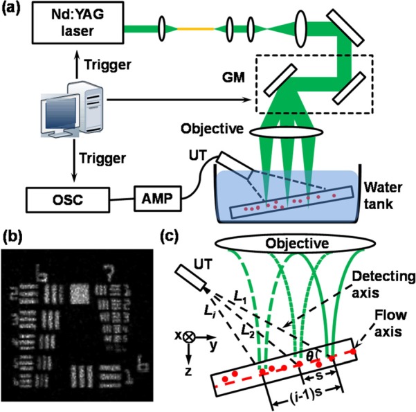
Experimental setup and principle of Doppler angle measurement. (a) Schematic diagram of LS-PAM. GM: galvanometer; UT: ultrasonic transducer; AMP: amplifier; OSC: oscilloscope; (b) LS-PAM image of an USAF 1951 resolution test target; (c) Illustration of the Doppler angle estimation in LS-PAM. θ: the angle between the transducer and the flow axes; L_i: the distance from the ith laser illumination position to the transducer tip; s: the interval between two adjacent PA illumination positions along the microtube.

A flow phantom was made to mimic a microvessel in our experiments. We made a suspension containing 0.4 × 10⁸ red dyed microspheres per milliliter (particle mean diameter: 6.0 μm; 15714-5, Polysciences) using distilled water. We added sodium polytungstate (71913, Sigma-Aldrich) to avoid sedimentation and TWEEN^® 20 (P1379, Sigma-Aldrich) at 1% volume to prevent aggregation. The suspension was filled in a polystyrene capillary tube (inner diameter: 250 μm; outer diameter: 500 μm; CTPS250-500, Paradigmoptics) driven by a syringe pump (A-99, Razel) at various flowing speeds. Although the microsphere volume density is low comparing with the hematocrit density in blood, previous studies suggested that PA Doppler methods verified by similar phantoms were well transferable to in vivo microcirculation measurements.^{2, 3}

Fig. 1c shows the principle to measure Doppler angle. Because of its small footprint, the ultrasonic detection can be considered as a point detector. The Doppler angle at a particular scanning position is defined as the angle θ between the detecting axis and the flow axis, as shown in Fig. 1c. Because the ultrasonic detector is kept stationary in LS-PAM, the geometrical relationship between optical illumination and ultrasonic detection changes during the data acquisition; as a result, the Doppler angle of the same flow can be different at different scanning positions. Using PA signals from multiple scanning positions along the flow, we have cos² θ = {[(i − 1) × s]² + L₁² − L_i²}/[2(i − 1) × s × L₁], where L_i is the distance from the ith illuminating position to the transducer tip. L_i can be obtained by multiplying the sound velocity in water (1.5 mm/μs) with the recorded time-of-flight (ToF) of the corresponding PA signals; s is the interval between two adjacent PA irradiation points. Similarly, we can describe cos²θ as cos²θ = {[s]² + L₁² − L₂²}/[2 × s × L₁] in a triangle defined by the first and second scanning positions with the lengths of the two sides L₁ and L₂. Provided these two equations, s can be solved as s² = [(i − 2) × L₁² + L_i² − (i − 1) × L₂²]/(i² − 3i + 2); hence, we can further solve θ after s is calculated. At least three consecutive illuminating points (i ≥ 3) are needed to calculate θ, while more illuminating points can be employed to improve the precision.

Fig. 2 shows the phantom results for measuring Doppler angles. We first fixed the angle between the axis of ultrasonic transducer and the microtube centerline at around 42° by mounting the transducer on a rotation stage (RSX-1, Newport) and the tube on a goniometer (GN05, Thorlabs). The flow speed was fixed at 13.5 mm/s at the syringe pump. The imaging acquisition took ∼3.3 s with 256 × 256 illuminating positions. Fig. 2a is the maximum amplitude projection (MAP) image of the tube along the x-y plane, from which we measured the inner diameter to be 241 ± 2.1 μm. Fig. 2b is the cross-sectional image of the tube along the y-z plane at the position highlighted in Fig. 2a. The slope of the imaged spheres cloud reflects the distance of the PA wave traveling from each illuminating position to the transducer tip. Fig. 2c shows the measured Doppler angle distribution along the dashed-line in Fig. 2a, which changes with the illuminating position as explained above. The angle θ in the tube center was 42.71 ± 0.14°, which agrees with the preset value. We then adjusted the tilting angle of the tube with respect to the transducer axis from 35° to 52° and compared the measured values with the preset values in Fig. 2d, where they agree with each other well.

Figure 2.

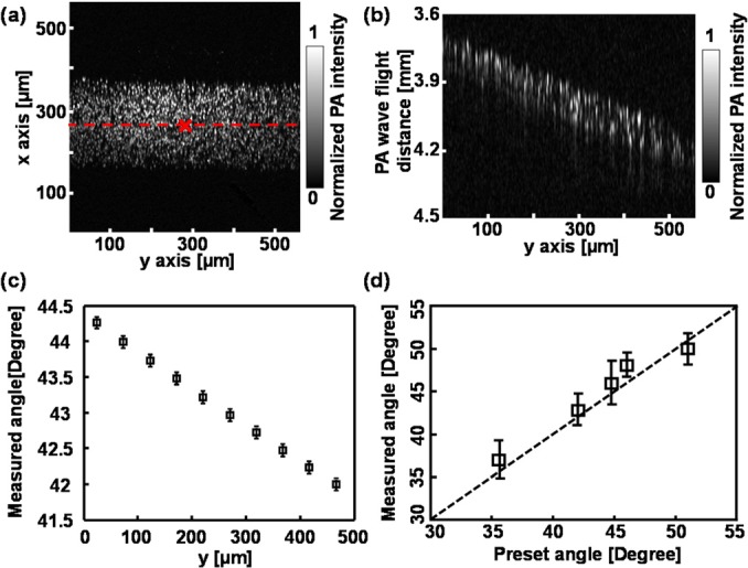
Experimental results of Doppler angle measurement. (a) LS-PAM image of a tube filled with optically absorption microspheres; (b) LS-PAM cross-sectional image along position highlighted by the dashed-line in panel (a); (c) Doppler angle distribution along the y axis; (d) comparison of preset and measured Doppler angles at the center, which is highlighted by the cross in panel (a), of the imaged tube.

Fig. 3a shows the principle to measure flow velocity along the detection axis. When a flowing optically absorbing microsphere travels through the optical focal region and is irradiated by two consecutive laser pulses, the two correspondingly detected PA signals (pulse 1 and pulse 2 in Fig. 3b) will have different ToFs if the flow axis is not perpendicular to the PA detection axis. As a result, the flowing velocity can be calculated by v = c × t_s/(T|cosθ|), where c is the sound speed; t_s is the ToF difference between the two consecutive PA signals; and T is the time interval between the two laser pulses.⁶ We determined the time shift t_s by performing temporal correlation of the two consecutive PA signals, as shown in Fig. 3c. The time (horizontal) shift, t_s, is the difference between the cross-correlation peak (CCP, between pulse 1 and pulse 2) and the auto-correlation peak (ACP, pulse 1 only). The sign of t_s reflects flow direction. We defined the positive direction as the flowing direction towards the ultrasonic detector, which has a negative time shift with respect to the auto-correlation peak. Because Brownian motion usually has a much longer diffusion time, its contribution to the cross-correlation variation can be reasonably neglected.^{3, 4}

Figure 3.

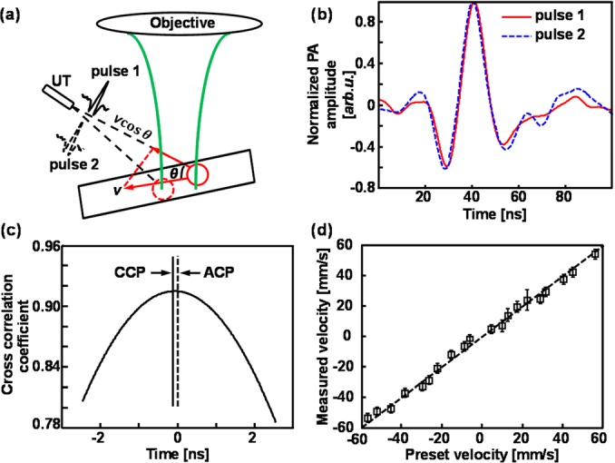
LS-PAM measurement of flow velocity. (a) Illustration of flow velocity measurement; (b) two sequential PA signals generated by the consecutive laser irradiations; (c) temporal correlation of the two consecutive PA waveforms shown in panel (b). CCP: cross-correlation peak between pulse 1 and pulse 2; ACP: auto-correlation peak of pulse 1 only; (d) comparison of preset and measured flow velocities at the center of the tube.

To measure absolute flow velocity in our microtube phantom, we first estimated the angle θ by recording the acoustic ToF from the multiple illumination points to the transducer tip. Then, we illuminated a selected position on the microtube with 20 laser pulses and calculated the flow velocity using every pair of PA signals generated by two consecutive pulses. We varied the flow speed and direction using the syringe pump; the measured and preset velocities are compared in Fig. 3d, where a good agreement can be observed.

The minimum measurable speed is determined by the laser PRR and the PA imaging SNR.^{3, 7} In this work, our PRR was 20 kHz, which corresponded with a minimum measurable speed of around 3.66 mm/s. The sensitivity (minimum detectable velocity) can be improved by decreasing the PRR at the expense of imaging speed or increasing the sampling rate of data acquisition instrument.^{6, 7} Another potential method to improve sensitivity without reducing PRR is to select every other or third pulse rather than consecutive pulses for cross-correlation. The maximum measurable speed is associated with PRR and the optical focus diameter,^{3, 4, 7} and is about 124.22 mm/s in the current experimental system. Here, we measured the flow speed up to 60 mm/s in both directions, which covers the range of blood flow in human retinal vessels.^{10, 11}

Because LS-PAM has a high lateral resolution, we further mapped the flow profile along the x axis, where the flow velocity in the tube was set at −49.5 mm/s. We first acquired a cross-sectional image along the z-x plane with 256A-lines (Fig. 4a). At each A-line position, we applied 40 illuminating pulses and calculated the corresponding velocity. Fig. 4b shows the distribution of flow velocity across the tube along the x-axis. We used a laminar flow model v(x) = v_max[1 − (x − x₀)²/r²] to fit the experimental date (Fig. 4b), where v_max is the flow velocity at the tube center, x₀ is the tube center coordinate, and r is the tube radius, respectively.⁷ The values of x₀ and r were obtained from Fig. 4a. Close to the tube boundary, the measured flow velocity became more unstable because of the low microsphere density and flow speed, as well as the degraded optical focusing caused by the tube wall. The structural image and the flow velocity profile in the tube cross-section were acquired in less than 0.52 s, and the total flow imaging duration, including the angle estimation, took less than 4 s.

Figure 4.

Flow velocity profile measured by LS-PAM. (a) Cross-sectional image of the microtube; (b) flow velocity profile along the x axis highlighted by the dashed-line in panel (a).

One question of interest is whether the velocity distribution along the z axis² will affect the Doppler measurement. During data acquisition, we carefully aligned the optical illumination to be around the tube center; and PAM only detected a volume average along the z axis due to its limited ultrasonic bandwidth. As a result, PA signals were generated from around the flow center. More importantly, we believe that the time shift obtained from the cross-correlation between consecutive PA signals reflects velocities of the fastest-moving spheres, which locate around the flow center. Under normal physiological condition, flowing red blood cells are shown to concentrate at the vessel center,¹² which suggests that our PAM Doppler method is applicable to in vivo blood flow measurement.

In summary, we demonstrated the feasibility of LS-PAM to measure absolute flow velocity in a vessel-mimicking phantom. Unlike the mechanical scanning PAM system,^{3, 7} LS-PAM delivered the illumination laser onto the sample by scanning the incident light with a galvanometer and detected the PA waves by a stationary unfocused ultrasonic transducer; therefore, this system is more applicable to retinal imaging because it can achieve fast imaging acquisition.^{8, 9} In the future, by combining Doppler flow imaging capability with multi-wavelength hemoglobin oxygen saturation imaging,¹³ we can potentially quantify the metabolic rate of oxygen at a high speed in retinal microcirculation system using LS-PAM alone.

References

- Fang H., Maslov K., and Wang L. V., Phys. Rev. Lett. 99, 184501 (2007). 10.1103/PhysRevLett.99.184501 [DOI] [PubMed] [Google Scholar]
- Yao J. and Wang L. V., J. Biomed. Opt. 15, 021304 (2010). 10.1117/1.3339953 [DOI] [PMC free article] [PubMed] [Google Scholar]
- Yao J., Maslov K., Shi Y., Taber L. A., and Wang L. V., Opt. Lett. 35(9), 1419 (2010). 10.1364/OL.35.001419 [DOI] [PMC free article] [PubMed] [Google Scholar]
- Chen S. L., Xie Z., Carson P. L., Wang X., and Guo L. J., Opt. Lett. 36(20), 4017 (2011). 10.1364/OL.36.004017 [DOI] [PMC free article] [PubMed] [Google Scholar]
- Sarimollaoglu M., Nedosekin D. A., Simanovsky Y., Galanzha E. I., and Zharov V. P., Opt. Lett. 36(20), 4086 (2011). 10.1364/OL.36.004086 [DOI] [PMC free article] [PubMed] [Google Scholar]
- Brunker J. and Beard P., J. Acoust. Soc. Am. 132(3), 1780 (2012). 10.1121/1.4739458 [DOI] [PubMed] [Google Scholar]
- Yao J., Maslov K., and Wang L. V., Technol. Cancer Res. Treat. 11(4), 301 (2012) 10.7785/tcrt.2012.500278. [DOI] [PMC free article] [PubMed] [Google Scholar]
- Jiao S., Jiang M., Hu J., Fawzi A., Zhou Q., Shung K. K., Puliafito C. A., and Zhang H. F., Opt. Express 18(4), 3967 (2010). 10.1364/OE.18.003967 [DOI] [PMC free article] [PubMed] [Google Scholar]
- Song W., Wei Q., Liu T., Kuai D., Burke J. M., Jiao S., and Zhang H. F., J. Biomed. Opt. 17(6), 061206 (2012). 10.1117/1.JBO.17.6.061206 [DOI] [PMC free article] [PubMed] [Google Scholar]
- Wang Y., Bower B. A., Izatt J. A., Tan O., and Huang D., J. Biomed. Opt. 12(4), 041215 (2007). 10.1117/1.2772871 [DOI] [PubMed] [Google Scholar]
- Nagahara M., Tamaki Y., Tomidokoro A., and Araie M., Invest. Ophthalmol. Visual Sci. 52(1), 87 (2011) 10.1167/iovs.09-4422. [DOI] [PubMed] [Google Scholar]
- Aarts P., van den Broek S., Prins G., Kuiken G., Sixma J., and Heethaar R., Arterioscler., Thromb., Vasc. Biol. 8(6), 819 (1988). 10.1161/01.ATV.8.6.819 [DOI] [PubMed] [Google Scholar]
- Liu T., Wei Q., Wang J., Jiao S., and Zhang H. F., Biomed. Opt. Express 2(5), 1359 (2011). 10.1364/BOE.2.001359 [DOI] [PMC free article] [PubMed] [Google Scholar]