MIXREGLS: A Program for Mixed-Effects Location Scale Analysis

Abstract

MIXREGLS is a program which provides estimates for a mixed-effects location scale model assuming a (conditionally) normally-distributed dependent variable. This model can be used for analysis of data in which subjects may be measured at many observations and interest is in modeling the mean and variance structure. In terms of the variance structure, covariates can by specified to have effects on both the between-subject and within-subject variances. Another use is for clustered data in which subjects are nested within clusters (e.g., clinics, hospitals, schools, etc.) and interest is in modeling the between-cluster and within-cluster variances in terms of covariates. MIXREGLS was written in Fortran and uses maximum likelihood estimation, utilizing both the EM algorithm and a Newton-Raphson solution. Estimation of the random effects is accomplished using empirical Bayes methods. Examples illustrating stand-alone usage and features of MIXREGLS are provided, as well as use via the SAS and R software packages.

1. Introduction

Mixed-effects regression models (aka hierarchical linear models, multilevel models) have become a primary method for analysis of longitudinal (Hedeker and Gibbons 2006; Verbeke and Molenberghs 2000) and clustered (Goldstein 2011; Raudenbush and Bryk 2002) data. A basic characteristic of these models is the inclusion of random effects into regression models in order to account for the influence of subjects or clusters on their nested observations. Here, we will focus on longitudinal data, but it should be understood that the methods and program can also be applied to clustered data. For longitudinal data, these random effects reflect each person’s growth or development across time, and the variance of these random effects indicate the degree of variation that exists in the population of subjects. Typically, the error variance, or the within-subjects (WS) variance, and the variance of the random effects, or the between-subjects (BS) variance, are treated as being homogeneous across subject groups or levels of covariates. However, these homogeneity of variance assumptions can be relaxed by modeling differences in variances, both between and within, across subject groups. The study of intra-individual variability has received increasing attention (Fleeson 2004; Hertzog and Nesselroade 2003; Martin and Hofer 2004; Nesselroade 2004); these articles describe many of the conceptual issues and some traditional statistical approaches for examining such variation.

Modern data collection procedures, such as ecological momentary assessments (EMA) and/or real-time data captures, have been developed to record the momentary events and experiences of subjects in daily life (Bolger, Davis, and Rafaeli 2003). These procedures yield relatively large numbers of subjects and observations per subject, and data from such designs are sometimes referred to as intensive longitudinal data (Walls and Schafer 2006). Such designs are in keeping with the “bursts of measurement” approach described by Nesselroade and McCollam (2000), who called for such an approach in order to assess intra-individual variability. Studies of this type are particularly amenable to examining intra-individual variation and to explain why subjects differ in variability rather than solely in mean level. In this article, one of our examples will be from a natural history study of adolescent smoking, using EMA, where interest was on determinants of the variation in the adolescents’ moods.

Hedeker, Mermelstein, and Demirtas (2008) described the mixed-effects location scale model as an extended random-intercept model in which log-linear (sub)models are included for both the WS and BS variance, allowing covariates to influence both sources of variation. Additionally, the model also includes a random subject effect to the WS variance specification. This permits the WS variance to vary at the subject level, above and beyond the influence of covariates on this variance. The correlation of the random scale and location effects is included in the model, yielding a more general and realistic specification for the random effects. In Hedeker et al. (2008), SAS PROC NLMIXED was used to estimate the model parameters. However, NLMIXED is rather slow to run and often requires excellent starting values to converge to a solution, particularly for the mixed-effects location scale model. Additionally, some data analysts find NLMIXED difficult to use, as it requires a higher degree of statistical programming knowledge than the average procedure in SAS. These considerations led to the development of the MIXREGLS (mixed-effects regression with location scale) program.

This article describes MIXREGLS for the analysis of repeated or clustered (conditionally) normally-distributed response variables using maximum likelihood and empirical Bayes estimation procedures. The full model is estimated in three sequential stages, each using Newton-Raphson, and the results of each stage are provided in the output. Prior to Stage 1, once the data are read in, 20 iterations are performed of the EM algorithm to estimate the parameters of a random intercept model (regression coefficients, BS variance, WS variance, and random location effects). These estimates are then used as starting values at Stage 1 to estimate the same parameters plus the BS variance effects. Then at Stage 2, WS variance effects are added, and finally at Stage 3 the random scale (and association between the random location and scale effects) is included. Estimates at each stage are used as starting values at the next stage, which improves the convergence of the final model. This also provides a way of assessing the statistical significance of the additional parameters in each stage via likelihood-ratio tests.

The organization of the article is as follows: Section 2 describes the mixed-effects location scale model, Section 3 presents details of MIXREGLS use, Section 4 illustrates application of MIXREGLS using two examples, and Section 5 discusses and summarizes the program. Estimation details are provided in Appendix A. The datasets that comprise the two examples are distributed with the program. The first is a traditional longitudinal study in which subjects are measured at six timepoints. The second example is an intensive longitudinal dataset incorporating EMA, in which subjects were measured, on average, 34 times during a weekly measurement period. Section 4 provides detailed instructions on MIXREGLS usage for these two examples, including explanation of the output, additional results files, how the program can be run via SAS, and running the program’s dynamic-link library (DLL) from R. Though the examples are both longitudinal in nature, in which observations are clustered within subjects, these methods and the program can also be applied to multilevel or hierarchical data in which subjects are nested within clusters (e.g., classrooms, schools, clinics, hospitals, etc.).

2. Mixed-effects location scale model

Consider the following mixed-effects regression model for the measurement y of subject i (i = 1, 2, …, N subjects) on occasion j (j = 1, 2, …, n_i occasions):

$$y_{\mathit{ij}}=x_{\mathit{ij}}^{⊺}\beta +v_i+{∊}_{\mathit{ij}},$$ (1)

where x_ij is the p × 1 vector of regressors (typically including a “1” for the intercept as the first element) and β is the corresponding p × 1 vector of regression coefficients. The regressors can either be at the subject level, vary across occasions, or be interactions of subject-level and occasion-level variables. In the multilevel terminology, subjects are at level 2, while the repeated observations are at level 1. Thus, the level-2 random subject effect ν_i indicates the influence of subject i on his/her repeated level-1 measurements. The population distribution of these random effects is assumed to be a normal distribution with zero mean and variance ${\sigma }_v^2$. The errors ∊_ij are also assumed to be normally distributed in the population with zero mean and variance ${\sigma }_{∊}^2$, and independent of the random effects. Here, ${\sigma }_v^2$ represents the BS variance and ${\sigma }_{∊}^2$ is the WS variance.

To allow covariates (i.e., regressors) to influence the BS and WS variances, we can utilize a log-linear representation, as has been described in the context of heteroscedastic (fixed-effects) regression models (Harvey 1976; Aitkin 1987), namely,

$${\sigma }_{v_{\mathit{ij}}}^2=\exp \left(u_{\mathit{ij}}^{⊺}\alpha \right),$$ (2)

$${\sigma }_{{∊}_{\mathit{ij}}}^2=\exp \left(w_{\mathit{ij}}^{⊺}\tau \right).$$ (3)

The variances are subscripted by i and j to indicate that their values change depending on the values of the covariates u_ij and w_ij (and their coefficients). The number of parameters associated with these variances does not vary with i or j. Both u_ij and w_ij would usually include a (first) column of ones for the reference BS and WS variances (α₀ and τ₀), respectively. Thus, the BS variance equals exp α₀ when all covariates u_ij equal 0, and is increased or decreased as a function of these covariates and their coefficients α. Specifically, for a particular covariate u*, if α* > 0, then the BS variance increases as u* increases (and vice versa if α < 0). The exponential function ensures a positive multiplicative factor for any finite value of α, and so the resulting variance is positive. It should be noted that an occasion-level variable, say u_ij, can alter the BS variance ${\sigma }_{v_{ij}}^2$ by making subjects more/less heterogenous across occasions. For example, in our modeling of mood in Section 4.3 the occasion-level variable “being alone (vs with others)” increases subject-level heterogeneity in mood. Thus, subjects are more alike in their mood responses when they are with others than when they are alone. The WS variance is modeled in the same way, allowing both subject- and occasion-level variables to influence how consistent/erratic a subject’s responses are. The coefficients in α and τ indicate the degree of influence on the BS and WS variances, respectively, and the ordinary random intercept model is obtained if α = τ = 0 for all covariates in u_ij and w_ij (i.e., excluding the reference variances α₀ and τ₀).

The WS variance can vary across subjects, above and beyond the effect of covariates, namely,

$${\sigma }_{{∊}_{\mathit{ij}}}^2=\exp (w_{\mathit{ij}}^{⊺}\tau +{\omega }_i),$$ (4)

where the random subject (scale) effectsω_i are distributed in the population of subjects with mean 0 and variance ${\sigma }_{\omega }^2$. The idea for this is akin to the inclusion of the random (location) effects in Equation 1, namely, covariates do not account for all of the reasons that subjects differ from each other. The ν_i parameters in Equation 1 indicate how subjects differ in terms of their means and the ω_i parameters in Equation 4 indicate how subjects differ in variation, beyond the effect of covariates. Taking logs in Equation 4 yields $\log \left({\sigma }_{{∊}_{ij}}^2\right)=w_{ij}\tau +{\omega }_i$, which indicates that if the distribution of ω_i is specified as normal, then the random effects serve as log normal subject-specific perturbations of the WS variance. In other words, the WS variances follow a log normal distribution at the subject level. The skewed, nonnegative nature of the log normal distribution makes it a reasonable choice for representing variances, and it has been used in many diverse research areas for this purpose (Fowler and Whitlock 1999; Leonard 1975; Renò and Rizza 2003; Shenk and Burnhamb 1998; Vasseur 1999).

In this model, ν_i is a random effect which influences a subject’s mean, or location, andω_i is a random effect which influences a subject’s variance, or (square of the) scale. Thus, the model with both types of random effects is dubbed a mixed-effects location scale model. These two random effects are correlated with covariance parameter σ_νω, which indicates the degree to which the random location and scale effects are associated with each other.

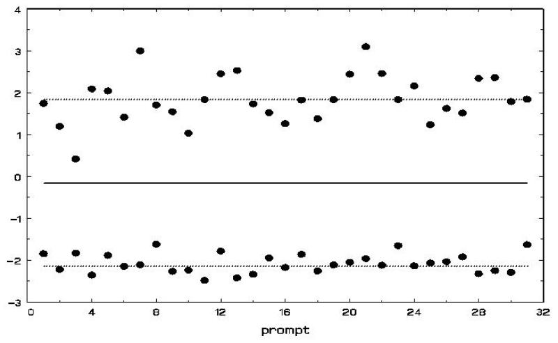
Visually, Figure 1 presents the pertinent details of the model. The average across all subjects is depicted by the solid horizontal line, and the lines of two subjects are presented as dotted lines. In a given dataset, there will be as many dotted lines as there are subjects, but for simplicity here we only plot two subjects. Also, for simplicity, consider all covariates as subject-varying only. The effect of covariates x on the mean response is represented by β; these effects either raise or lower the solid line as a function of the covariates. Each dotted line represents a person’s random location effect ν_i, which indicate how a subject deviates from the mean response. In Figure 1, one subject is above and another subject is below the mean line. The heterogeneity in these dotted lines is indicative of BS variance: if the dotted lines are close together then there is not much subject heterogeneity, conversely if the dotted lines are spread out then more heterogeneity is indicated. The effect of covariates u on this heterogeneity is represented in the model as α. The degree of variation of a person’s data points around their line is the WS variance. If the points are quite close to a subject’s line, then that subject has low WS variance (e.g., the lower subject in Figure 1). Conversely, if a subject’s data points vary greatly around that person’s line then there is more WS variation (e.g., the upper subject in Figure 1). Covariates w influence the WS variation through the coefficients τ. Finally, the model posits that covariates do not explain all of a subject’s WS variance by including the random scale effect ω_i.

Figure 1.

A visual representation of the mixed-effects location scale model.

2.1. Standardization of random effects

It is convenient to represent the random effects in standardized form (i.e., as standard normals). For this, we can use the Cholesky factorization (Bock 1975).

$$\left[\begin{array}{c}\hfill v_i\hfill \\ \hfill w_i\hfill \end{array}\right]=\left[\begin{array}{cc}\hfill s_{1\mathit{ij}}\hfill & \hfill 0\hfill \\ \hfill s_{2\mathit{ij}}\hfill & \hfill s_{3\mathit{ij}}\hfill \end{array}\right]\left[\begin{array}{c}\hfill {\theta }_{1i}\hfill \\ \hfill {\theta }_{2i}\hfill \end{array}\right]=\left[\begin{array}{cc}\hfill {\sigma }_{v\mathit{ij}}\hfill & \hfill 0\hfill \\ \hfill {\sigma }_{vw}∕{\sigma }_{v\mathit{ij}}\hfill & \hfill \sqrt{{\sigma }_w^2-{\sigma }_{\mathit{vw}}^2∕{\sigma }_{v_{\mathit{ij}}}^2}\hfill \end{array}\right]\left[\begin{array}{c}\hfill {\theta }_{1i}\hfill \\ \hfill {\theta }_{2i}\hfill \end{array}\right]$$ (5)

Here, we include the subscripts i and j on the Cholesky elements because the BS variance ${\sigma }_{v_{ij}}^2$ is allowed to vary by subjects and/or occasions. The model can now be written as

$$y_{\mathit{ij}}=x_{\mathit{ij}}^{⊺}\beta +s_{1\mathit{ij}}{\theta }_{1i}+{∊}_{\mathit{ij}}$$ (6)

where $s_{1ij}={\sigma }_{v_{ij}}=\sqrt{\exp \left(u_{ij}\alpha \right)}$, and the errors ∊_ij have variance given by

$${\sigma }_{{∊}_{\mathit{ij}}}^2=\exp (w_{\mathit{ij}}^{⊺}\tau +s_{2\mathit{ij}}{\theta }_{1i}+s_{3\mathit{ij}}{\theta }_{2i}).$$ (7)

2.2. Alternative formulation for association of location and scale

Suppose that instead of allowing the location and scale random effects to be correlated, we assume that they are independent (i.e., σ_νω = 0, and therefore s_2ij = 0), but that the location random effect θ_1i explicitly influences the WS variance. In this case, the WS variance could be expressed as

$${\sigma }_{{∊}_{\mathit{ij}}}^2=\exp (w_{\mathit{ij}}^{⊺}\tau +{\tau }_l{\theta }_{1i}+{\sigma }_{\omega }{\theta }_{2i}).$$ (8)

where the regression coefficient τ_l represents the (linear) influence of the location random effect θ_1i on the (log of the) WS variance. These two models of the WS variance are essentially the same, although in Equation 7 the parameter s_2ij is indicative of the covariance between the random location and scale effects, whereas in Equation 8 the parameter τ_l represents the effect of the random location effect on the WS variance. Also, the Cholesky element s_3ij in Equation 7 is replaced by the (simpler) square root of the random scale σ_ω in Equation 8. We have merely shifted from a correlation-like association between the mean and variance to a regression setting in which the mean influences the variance. Although equivalent in the present case, the latter representation can be more easily generalized to represent various forms of the relationship between the random location effect and the WS variance. For example, one can easily extend the model to allow for a quadratic relationship, namely,

$${\sigma }_{{∊}_{\mathit{ij}}}^2=\exp (w_{\mathit{ij}}^{⊺}\tau +{\tau }_l{\theta }_{1i}+{\tau }_q{\theta }_{1i}^2+{\sigma }_{\omega }{\theta }_{2i}).$$ (9)

A quadratic relationship would seem to be useful for rating scale data with ceiling and/or floor effects, where subjects that have mean levels at either the maximum or minimum value of the rating scale also have near-zero variance. For example, if the rating scale goes from 1 to 10, then any subject with a mean level near either 1 or 10 would almost certainly have a very small variance, giving rise to the potential for a quadratic relationship between the mean and variance. In this regard, MIXREGLS allows for three possibilities: (1) no association (τ_l = τ_q = 0); (2) linear association only (τ_l ≠ 0, τ_q = 0); and (3) linear and quadratic association (τ_l ≠ 0, τ_q ≠ 0). For a given program run, the user can select one of these three possibilities using the NCOV option, described in Section 3.

2.3. Intraclass correlation

The standardized random effects θ_1i and θ_2i are both normally distributed with mean 0 and variance 1, and are independent of each other. The expectation of y_ij, E(y_ij), is simply $x_{ij}^{⊺}\beta$. For the situation in which the random location θ_1i has a quadratic effect on the WS variance (i.e., τ_q ≠ 0), the variance of y_ij varies as a function of the random location effect. However, for the simpler situation in which τ_q = 0, the variance of y_ij is given by

$$V\left(y_{\mathit{ij}}\right)=\exp \left(u_{\mathit{ij}}^{⊺}\alpha \right)+\exp \left(w_{\mathit{ij}}^{⊺}\tau +\frac{1}{2}\left[{\tau }_l^2+{\sigma }_{\omega }^2\right]\right).$$ (10)

The covariance for any two observations nested within the same subject i equals

$$C(y_{\mathit{ij}},y_{{\mathit{ij}}^{\prime }})={\sigma }_{v_{\mathit{ij}}}^2=\exp \left({\mathit{u}}_{\mathit{ij}}^{\prime }\alpha \right)\text{for}j\ne j^{\prime }.$$ (11)

Expressed as a correlation, this yields the intraclass correlation (ICC), denoted as r_ij,

$$r_{\mathit{ij}}=\frac{\exp \left(u_{\mathit{ij}}^{⊺}\alpha \right)}{\exp \left(u_{\mathit{ij}}^{⊺}\alpha \right)+\exp \left(w_{\mathit{ij}}^{⊺}\tau +\frac{1}{2}[{\tau }_l^2+{\sigma }_{\omega }^2]\right)}.$$ (12)

Note that the ICC, which represents the proportion of total unexplained variation that is at the subject level, can be obtained for specific values of the covariates u_ij and w_ij. Thus, based on the current model, the ICC is allowed to vary as a function of both time-varying and time-invariant covariates.

3. Program description and usage

MIXREGLS uses maximum likelihood to estimate the model parameters β, α, τ, τ_l, τ_q, and σ_ω. Specifically, it uses the Newton-Raphson algorithm to iteratively achieve the likelihood solution, with integration over the random effects done using numerical quadrature. The quadrature points and weights can be adapted to each person’s data. Upon convergence, estimates of the random effects (θ_1i and θ_2i) are obtained using empirical Bayes methods. Details on estimation are provided in Appendix A.

MIXREGLS was written in standard Fortran 95 for Windows-based computers. It can be run in batch mode using the executable file mixreglsb.exe, or accessed via the DLL file mixregls.dll; an example of this latter type of usage within R will be given in Section 4.2. Here, we will first describe batch processing use. Program instructions must be stored in the file mixregls.def, the contents of which will be described below. MIXREGLS makes use of the following files: mixregls.def (definition file), filename.dat (input data file), filename.out (main output file), and filename.def (definition file to be saved).

3.1. Structure of filename.dat

This file contains all data read by the program. It is read in free format and must be a standard text (ASCII) file with no hidden characters or word processing format codes. Variable fields must be separated by one or more blanks. The data are assumed to consist of multiple level-1 observations within a level-2 unit, for example, in the longitudinal setting there are repeated observations (level 1) within subjects (level 2). There must be a level-2 id variable for each record, and the data must be sorted by this variable. The repeated measurements of a subject often take up as many records in this file as there are measurements for that subject. An exception to this is when the variables for a subject on a given occasion comprise more than one physical record, say two records. In this case, the repeated measurements of a subject take up twice as many records in the file as there are measurements for that subject. Also, if missing value codes are utilized, each subject may have data on the same number of records, but some records will contain missing value codes for some (or all) of the variables.

The fields of variables that are read in, separated by one or more blanks, usually consist of the id variable, the dependent variable, and covariates. (the order of variables does not matter). The covariates include the regressors for the mean submodel (x), BS variance submodel (u), and WS variance submodel (w); the covariates in these submodels (i.e., x, u, and w) can be the same or different. All variables are read as real numbers with the exception of the id variable which is read as integer. All missing data must have a numeric missing value code, in particular, blank fields or periods are not acceptable as missing value codes. There is no need to include a column of ones in the dataset for the intercept(s), as the program can include intercepts for all submodels (though this can be changed using the PNINT, RNINT, and SNINT options, see below).

3.2. Structure of mixregls.def

This file contains specifications that determine the statistical model to be fit to the data in filename.dat. Except where noted, this file is read in free format. The filename and extension (mixregls.def) must be used, and should be in the same directory as the program mixreglsb.exe. This file needs to be created with an editor and saved in text format; one then double-clicks on the mixreglsb.exe file (or types mixreglsb at the command prompt) to run the program. Below are the specifications, and their optional values, that are necessary.

• Line 1 – title of 72 characters

• Line 2 – subtitle of 72 characters

• Line 3 – filename.dat (input data file)

• Line 4 – filename.out (main output file)

• Line 5 – filename.def (definition file; the contents of mixregls.def are saved to this file)

• Line 6 – NVAR P R S PNINT RNINT SNINT CONV NQ AQUAD MAXIT MISS STD NCOV

  • NVAR = number of variables to read from filename.dat
  • P = number of covariates for the mean submodel
  • R = number of covariates for the BS variance submodel
  • S = number of covariates for the WS variance submodel
  • PNINT = 0 (the mean submodel should include an intercept) or 1 (the mean submodel should not include an intercept)
  • RNINT = 0 (the BS variance submodel should include an intercept) or 1 (the BS variance submodel should not include an intercept)
  • SNINT = 0 (the WS variance submodel should include an intercept) or 1 (the WS variance submodel should not include an intercept)
  • CONV = convergence criterion (usually 0.0001 or 0.00001); when all of the parameter first derivatives are smaller than this level, the algorithm has converged to a solution
  • NQ = number of quadrature points
  • AQUAD = 0 (non-adaptive quadrature) or 1 (adaptive quadrature)
  • MAXIT = maximum number of iterations; if the program does not converge by this number, the program stops and prints out the current estimates
  • MISS = 0 (no missing values) or 1 (missing values)
  • STD = 0 (covariates will not be standardized) or 1 (all covariates will be standardized with mean 0 and variance 1)
  • NCOV = 0 (no association between the random location and WS variance), or 1 (only linear association between the random location and WS variance), or 2 (linear and quadratic association between the random location and WS variance)

• Line 7 – two parameters: fields of the id variable and the dependent variable in filename.dat

• Line 8 – P parameters: field(s) of mean covariates in filename.dat

• Line 9 – R parameters: field(s) of BS variance covariates in filename.dat

• Line 10 – S parameters: field(s) of WS variance covariates in filename.dat

• Line 11 – 8 character label for the dependent variable

• next line(s) – P labels for mean covariates in 8 character width fields (maximum of 10 labels per line)

• next line(s) – R labels for BS variance covariates in 8 character width fields (maximum of 10 labels per line)

• next line(s) – S labels for WS variance covariates in 8 character width fields (maximum of 10 labels per line)

• If MISS=1 then the next lines are required and list the numeric missing value codes

• next line – missing value code for the dependent variable

• next line – P missing value codes, separated by blanks, for the mean covariates

• next line – R missing value codes, separated by blanks, for the BS variance covariates

• next line – S missing value codes, separated by blanks, for the WS variance covariates

Upon program completion, the file specified on Line 4 (filename.out) will contain the results of the analysis. The contents of this file will be described for the two examples in Section 4. Additionally, for a given run, four additional files are created by MIXREGLS: mixregls.its, mixregls.re1, mixregls.re2, and mixregls.est. The file mixregls.its contains iteration-specific details including the likelihood value and the largest correction and derivative of the parameter estimates. The information that is included in this file is also displayed on the screen while the program is running. The file mixregls.re1 contains standardized (level-1) residuals, while mixregls.re2 contains the empirical Bayes estimates of the random effects (these are sometimes referred to as the level-2 residuals). As mentioned, MIXREGLS fits the mixed-effects location scale model in three stages. At the first stage, only the mean and BS variance covariate effects are estimated. At the second stage, the WS variance covariate effects are added. Finally, at stage three, the random scale effects are included. mixregls.re1 and mixregls.re2 contain results for all three stages. For the first two stages, four pieces of information are given in mixregls.re2: level-2 id, the number of level-1 observations for the level-2 unit, empirical Bayes estimate of the random location effect, and the posterior variance associated with the location effect. For stage three, which includes random location and scale effects, both empirical Bayes estimates of the location and scale effects are listed in mixregls.re2, followed by the posterior variance-covariance matrix associated with the random effects (in order: location variance, location scale covariance, scale variance). The file mixregls.est contains a listing of the deviance (−2 ln L), number of iterations, MAXIT (i.e., maximum number of iterations), estimates (in the order P, R, S), and standard errors for all three model stages, respectively.

3.3. Some MIXREGLS errors

There are a few errors which can prevent MIXREGLS from running correctly, or even running at all. All information in the filename.dat file needs to be numeric, so any alphanumeric variables in this file will cause the program to fail. Also, missing values left as blank fields, and not given a specified numeric missing value code, may cause the program to fail or to estimate a model which is incorrect from the user’s perspective. To see if this is causing a problem, the user can check the correctness of each variable’s descriptive statistics (mean, minimum, maximum, and standard deviation) listed in the output file filename.out. If these descriptive statistics are incorrect, the data are not being read into the program correctly and a common reason is that missing values are being left as blank fields in the data file.

If the program “blows up,” or does not converge to the solution by the maximum number of iterations (MAXIT), one thing to try is to standardize the covariates by setting STD = 1. This will ensure that all of the covariates, for all submodels, are on the same numerical scale with mean 0 and variance 1. Specifically, the standardized covariate z_x is obtained as z_x = (x − x̄)/s_x, where x̄ and s_x are the mean and standard deviation of x based on all of the observations.

For models that do not converge properly, another thing to try is to increase the number of quadrature points (NQ) and/or switch to adaptive quadrature (i.e., set AQUAD = 1). It may be, for example, that specifying 10 points will not lead to convergence, while specifying 15 points does. Estimation of the final model stage, where the random scale effect is included, can be sensitive to the number of quadrature points. If after increasing the number of quadrature points to a very large number (say NQ = 31 or 41), problems still exist, it may be that the random-effect scale variance cannot be reliably estimated. In this case, a model without random scale may be warranted (i.e., stage 1 or 2).

4. Examples of mixed-effects location scale regression

MIXREGLS can estimate a variety of models for clustered and longitudinal data. It is especially useful for intensive longitudinal data, where subjects might have 30 or 40 (or more) observations, and interest is on examining the heterogeneity associated with the many responses. Here, we will present two examples that highlight MIXREGLS use for a typical longitudinal dataset and also for an EMA dataset. These two examples illustrate some of the ways in which MIXREGLS can be used, and the results that are obtained from the program.

4.1. Longitudinal analysis with random location and scale effects

A psychiatric study described in Reisby, Gram, Bech, Nagy, Petersen, Ortmann, Ibsen, Dencker, Jacobsen, Krautwald, Sondergaard, and Christiansen (1977) focused on the longitudinal responses of 66 depressed inpatients. In this study, subjects were diagnosed with either endogenous (N = 37) or non-endogenous (N = 29) depression, and were rated with the Hamilton depression rating scale (hamdep) weekly for a total of six weeks. Although the total number of subjects in this study was 66, the number of subjects with all measures at each of the weeks fluctuated: 61 at week 0 (baseline), 63 at week 1, 65 at week 2, 65 at week 3, 63 at week 4, and 58 at week 5. For this illustration, we focus on the following aspects of the study: is there evidence of differential improvement across time between endogenous and non-endogenous patients, and do the groups exhibit differential BS and WS heterogeneity. Additional analyses of this dataset can be found in Hedeker and Gibbons (1996).

The model fit to the hamdep scores includes a random subject intercept (i.e., random location effect), as well as a time effect, group effect (endogenous or non-endogenous) and a group by time interaction to examine whether these two groups of patients differed in terms of their initial severity and improvement across time. Additionally, we will investigate whether the two groups have different WS and BS variances, and allow the WS variance to change across time. A matrix representation of the model for subject i is given by

$$\left[\begin{array}{c}\hfill {\text{hamdep}}_{i0}\hfill \\ \hfill {\text{hamdep}}_{i1}\hfill \\ \hfill {\text{hamdep}}_{i2}\hfill \\ \hfill {\text{hamdep}}_{i3}\hfill \\ \hfill {\text{hamdep}}_{i4}\hfill \\ \hfill {\text{hamdep}}_{i5}\hfill \end{array}\right]=\left[\begin{array}{cccc}\hfill 1\hfill & \hfill 0\hfill & \hfill {\text{endog}}_i\hfill & \hfill {\text{endog}}_i\times 0\hfill \\ \hfill 1\hfill & \hfill 1\hfill & \hfill {\text{endog}}_i\hfill & \hfill {\text{endog}}_i\times 1\hfill \\ \hfill 1\hfill & \hfill 2\hfill & \hfill {\text{endog}}_i\hfill & \hfill {\text{endog}}_i\times 2\hfill \\ \hfill 1\hfill & \hfill 3\hfill & \hfill {\text{endog}}_i\hfill & \hfill {\text{endog}}_i\times 3\hfill \\ \hfill 1\hfill & \hfill 4\hfill & \hfill {\text{endog}}_i\hfill & \hfill {\text{endog}}_i\times 4\hfill \\ \hfill 1\hfill & \hfill 5\hfill & \hfill {\text{endog}}_i\hfill & \hfill {\text{endog}}_i\times 5\hfill \end{array}\right]\left[\begin{array}{c}\hfill {\beta }_0\hfill \\ \hfill {\beta }_1\hfill \\ \hfill {\beta }_2\hfill \\ \hfill {\beta }_3\hfill \end{array}\right]+\left[\begin{array}{c}\hfill {\theta }_{1i}\hfill \\ \hfill {\theta }_{1i}\hfill \\ \hfill {\theta }_{1i}\hfill \\ \hfill {\theta }_{1i}\hfill \\ \hfill {\theta }_{1i}\hfill \\ \hfill {\theta }_{1i}\hfill \end{array}\right]\left[{\sigma }_{vi}\right]+\left[\begin{array}{c}\hfill {∊}_{i0}\hfill \\ \hfill {∊}_{i1}\hfill \\ \hfill {∊}_{i2}\hfill \\ \hfill {∊}_{i3}\hfill \\ \hfill {∊}_{i4}\hfill \\ \hfill {∊}_{i5}\hfill \end{array}\right]$$

Here, the grouping variable (endog) is a dummy-coded variable indicating whether a subject is endogenous (endog=1) or non-endogenous (endog=0). For the trend in hamdep means across time, the model includes a linear effect of week (coded sequentially from 0 to 5) and a group by (linear) week interaction. In terms of the variance modeling, we allow

$${\sigma }_{v_i}^2=\exp ({\alpha }_0+{\alpha }_1{\text{endog}}_i),$$ (13)

for the BS variance, and

$${\sigma }_{{∊}_{\mathit{ij}}}^2=\exp ({\tau }_0+{\tau }_1{\text{week}}_j+{\tau }_2{\text{endog}}_i+{\tau }_l{\theta }_{1i}+{\sigma }_{\omega }{\theta }_{2i}),$$ (14)

for the WS variance. Thus, the parameters α₁ and τ₂ represent differences between the groups in terms of the BS and WS variances, respectively. Additionally, τ₁ characterizes the change in the error (WS) variance across time, τ_l is the effect of a subject’s random location effect on their WS variance, and σ_ω is the standard deviation of the random subject scale effect.

Although the above matrix representation is for a subject with data at all six timepoints, this is not a requirement. If a subject’s data are missing or incomplete, then they would simply contribute less than six observations in the dataset, or their missing data would be coded with numeric missing value codes, which would be identified in the mixregls.def file prior to the statistical analysis. For this first example, the following is the order and names of the variables in the the dataset riesby_example.dat: (subject’s) id, hamdep, week, endog, and endweek (the product of endog and week). There are missing value codes (−9) for some subjects at specific timepoints; the data from these timepoints are not used in the analysis, however data from these subjects at other timepoints, where there are no missing data, are used in the analysis. Thus, for inclusion into the analysis, a subject’s data (both the dependent variable and all model covariates being used in a particular analysis) at a specific timepoint must be complete. The number of repeated observations per subject then depends on the number of timepoints for which there are non-missing data for that subject. As MIXREGLS uses full likelihood estimation, described in Appendix A, it provides valid inference for incomplete data under missing at random (MAR) assumptions (Little and Rubin 2002).

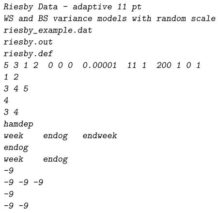
Covariates are specified for three submodels: the mean, the BS variance, and the WS variance submodels. If the options PNINT, RNINT, and SNINT are all set to zero, then the program will include intercepts for all submodels. This is the usual case and what will be specified here. Based on the model described above the following covariates will be specified; mean: week, endog, endweek; BS variance: endog; WS variance: week, endog. The dataset to be read contains five variable fields, with id (field 1), hamdep (field 2), week (field 3), endog (field 4), and endweek (field 5). The field number is used to identify these variables in the mixregls.def file for this model, which is listed below.

Note that even though missing values are coded only for the dependent variable in the input data file, numeric missing value codes must be specified in the mixregls.def file for all model variables (if MISS=1). In this case, the value −9 was specified for all variables since for the dependent variable this value is the correct missing value code, while for all other variables (week, endog, endweek) this value was never observed. Other options that are specified in this mixregls.def file: a convergence criterion of 0.00001, 11-point adaptive quadrature, a maximum number of iterations set at 200, no standardization of model covariates, and a linear effect of a subject’s location effect on the (log of their) WS variance.

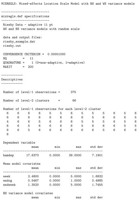
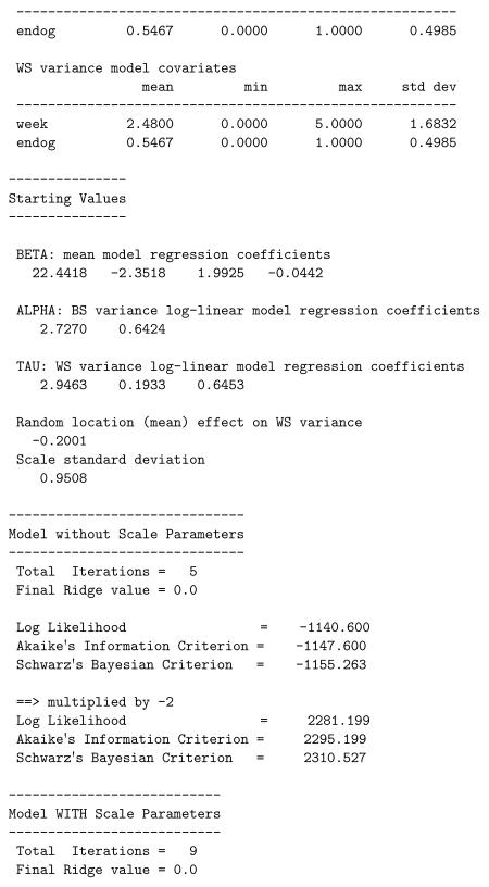
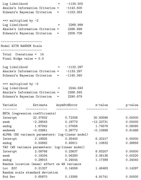
The results for the model are written to the file riesby.out and are listed below. Here, for space, we have removed the parameter estimates associated with stages 1 and 2. The first part of the output is a list of some of the information given in the mixregls.def file. Then, descriptive information about the dataset is provided: the number of level-1 observations, number of level-2 observations, and the number of level-1 observation for each level-2 cluster. Means, minimums, maximums, and standard deviations for all variables used in the analysis are listed. These descriptive statistics should be checked to confirm that the program has read the data correctly, otherwise the results of the subsequent analyses are presumably incorrect. Following the descriptives, starting values for all parameters are listed. Using code from the MIXREG program (Hedeker and Gibbons 1996), the program performs 20 iterations of the EM algorithm for a random-intercepts model. This provides excellent starting values for the regression coefficients, BS and WS variances, and random location effects.

Following the starting values, results for each of the three model stages are printed out. For each, the output includes the number of iterations required for convergence, the final ridge value, the log-likelihood value at convergence, and penalized versions of the log-likelihood value (i.e., Akaike’s information criterion and Schwarz’s Bayesian criterion). These likelihood values are also listed multiplied by −2 to aid in performing likelihood-ratio tests and/or model selection. The ridge is an adjustment made to the diagonal of the Hessian matrix (matrix of second derivatives) if the program encounters a non-increasing likelihood or some other indication of numerical difficulty. This adjustment often improves the chances of convergence. Specifically, the diagonal of the Hessian matrix is multiplied by one plus the ridge value at each iteration. Thus, if the ridge value equals zero, there is no adjustment, however if the ridge value is greater than zero, then the diagonal elements of the Hessian matrix are increased. Increasing the diagonal elements of the Hessian matrix decreases the corrections or step sizes for each parameter in the iterative Newton-Raphson algorithm, thereby tending to stabilize the estimation procedure. At present, the ridge starts at zero (stage 1), 0.1 (first few iterations of stage 2), and 0.2 (first few iterations of stage 3), and is increased by 0.1 each time that difficulties are encountered. The ridge is then set back to zero if, after several iterations, the computations seem to be going smoothly. Also, at convergence, the ridge is set back to zero in order to obtain the correct standard errors for the model parameters, however the listing of the final ridge value indicates its value prior to being reset to zero. As such, the listed ridge value is indicative of the degree of computational difficulty that the program encountered.

All three stages include the covariate effects on the mean, but vary in terms of the variance effects and the random scale: (stage 1) a model with BS variance effects but no WS variance effects; (stage 2) a model with both BW and WS variance effects but no random scale effect; (stage 3) the full model including random scale effects and association of the random location and scale effects. Likelihood ratio tests can be used to compare these three model stages: ${\chi }_2^2$ = 2281.199 − 2268.999 = 12.2 comparing stages 1 and 2, and ${\chi }_2^2$ = 2268.999 − 2244.593 = 24.406 comparing stages 2 and 3. Thus, there are significant WS variance effects and subject differences of scale. Interpreting the final model stage, we see that there is a significant negative time effect in the mean model, indicating that depression scores are decreasing across time. The two groups (non-endogenous and endogenous) do not seem to differ in terms of either the BS or WS variance, while the WS variance does increase with study week. Thus, within a subject, the depression scores are more variable around his/her linear trajectory as the study progresses. There is significant subject variation in scale, indicating that subjects vary in terms of the dispersion of their depression scores around their linear trajectory, over and above the significant effect of study week. Finally, the linear random location effect on the log of the WS variance is non-significant.

Parameter estimates file – mixregls.est

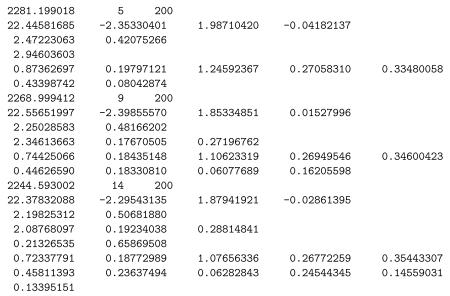
Following program termination, MIXREGLS writes out, to the file mixregls.est, information about the model fit and parameter estimates for each of the three stages, in order. The contents of this file can be read in by another program to, say, produce graphs of the parameter estimates or perform additional calculations. For the analysis of the Riesby data, the contents of mixregls.est are listed below.

The first line corresponding to each stage lists the deviance (−2 ln L), number of iterations required for convergence, and the maximum number of iterations specified (MAXIT in the mixregls.def file). Then, the parameter estimates are listed in the following order: regression coefficients $\widehat{\beta }$ (all stages), BS variance effects $\widehat{\alpha }$ (all stages), WS variance effects $\widehat{\tau }$ (stages 2 and 3), and for stage 3 only: random location ${\widehat{\tau }}_l$ and ${\widehat{\tau }}_q$ (depending on the NCOV specifcation) and random scale ${\widehat{\sigma }}_{\omega }$ parameters. Each set of estimates are written on new lines with a maximum of five estimates per line. The standard errors associated with all parameter estimates are then listed in (the same) order, however not on new lines for the different sets, but sequentially with five standard errors per line.

Empirical Bayes estimates – mixregls.re2

MIXREGLS uses empirical Bayes (EB) estimation for the random effects, and upon program termination, the estimates are automatically saved in the file mixregls.re2. This file contains estimates for all three model stages, and they are listed in order. In the file, there are lines with labels that precede the numeric results of each stage. For example, for the first two stages, four pieces of information are given on each line: the subject’s id, the number of repeated observations associated with the subject, the empirical Bayes estimate of the random subject (location) effect, and the posterior variance associated with the random subject effect. The line of labels in the file that precedes these results is “id, nobs, EB mean, EB var.” For stage three, which includes random location and scale effects, there are two lines per subject. The first contains the subject id, the number of repeated observations associated with the subject, and empirical Bayes estimates of the random subject location and scale effects. The second line lists the posterior variance-covariance matrix associated with the random subject effects (in order: location variance, location scale covariance, scale variance). The line of labels that precedes these results is “id, nobs, EB mean vector, EB variance-covariance.”

For the Riesby data, the EB estimates of scale (denoted ${\tilde{\theta }}_{2i}$) were sorted, and Table 1 lists the two subjects with the highest and lowest scale estimates. Also listed are the observed hamdep values for these subjects across time, abbreviated as hd0, … hd5. As can be seen, the two subjects with the highest scale estimates do not follow a linear pattern across time. In particular, the hamdep values at week 1 are quite aberrant relative to the other values across time. One wonders if these are correct values, or perhaps if they are coding errors. Given that this particular study was conducted well in the past, it is impossible to say. However, for more current studies, it seems that these scale estimates can be used to detect unusual patterns of responses and perhaps coding errors. Turning to the subjects with the lowest scale estimates, these are both subjects with near-perfect linear downward trajectories. Thus, subjects with the lowest scale estimates are those with responses that mimic the pattern of the estimated population mean model estimates, which in the present case is a downward linear trend across time. These scale estimates can then be used to identify “ideal” cases, or those subjects that behave most like the average in the population.

Table 1.

The data of the two highest and lowest scale estimates (${\tilde{\theta }}_{2i}$) from analysis of the Riesby data.

id	${\tilde{\theta }}_{2i}$	hd0	hd1	hd2	hd3	hd4	hd5
606	1.585	19	33	12	12	3	1
505	1.532	21	11	18	0	0	4
335	−1.317	21	21	18	15	12	10
308	−1.365	22	21	18	17	12	11

4.2. Running MIXREGLS from R

MIXREGLS can also be run from R via a dynamic-link library (DLL). Lemmon and Schafer (2005) describe creation of a DLL from Fortran code, and how the DLL can be accessed by R and other software programs. For MIXREGLS, the DLL file mixregls.dll, an R function file mixregls_function.r, and the R syntax file mixregls_run.r are distributed with the program. Additionally, the R package Formula (Zeileis and Croissant 2010) must be installed. Together, these files and package can be used to yield the same analysis of the Riesby data as in the previous section.

The R syntax file mixregls_run.r includes the following. First, the DLL file is loaded and checked to ensure that it is loaded.

R> dyn.load(“mixregls.dll”)

R> is.loaded(“mixreglsr”)

Then, the R function file is accessed.

R> source(“mixregls_function.r”)

The data are read in, variables with missing value codes of −9 are specified as not available, and a summary of the data are listed.

R> indata <- read.table(“riesby_example.dat”, header=F, + col.names=c(“id”,“hamdep”,“week”,“endog”,“endweek”), + na.strings=“−9”)

R> summary(indata)

The DLL is run using the using the R function mixregls.combined (which is defined in the file mixregls_function.r).

R> mixregls.results = mixregls.combined(hamdep ~ endog+week+endweek + | endog | endog+week, id=“id”, data=indata)

The dependent variable is specified as hamdep and the covariates are listed sequentially for the mean, BS variance, and WS variance submodels separated by the character |. If any of the three submodels had no covariates, but only an intercept, then a value of 1 should be provided, for example:

R> mixregls.results = mixregls.combined(hamdep ~ endog+week+endweek + | 1 | endog+week, id=“id”, data=indata)

would only include an intercept in the BS variance submodel. Results are listed for all three stages using the print.mixregls_output function (included in mixregls_function.r).

R> print.mixregls_output(mixregls.results)

Results of each stage can also be accessed: the deviance (dev), mean submodel estimates (beta), BS variance submodel estimates (alpha), WS variance submodel estimates (tau), and all standard errors (se). A numerical suffix of 1, 2, or 3 indicates the stage. For example, to list the mean submodel estimates for stage 1, the following statement would be issued.

R> mixregls.results$beta1

For stage 3, estimates of the parameters associated with the inclusion of the random scale effect (τ_l, τ_q, and σ_ω) are returned (spar); to list these the following statement would be used.

R> mixregls.results$spar3

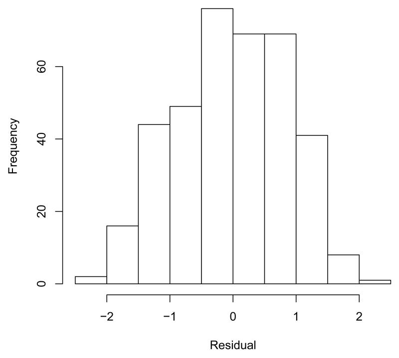
For all three stages, standardized residuals (zerr) are also returned from the DLL. For stage 3, these are plotted in a histogram and presented in Figure 2.

Figure 2.

Histogram of standardized model residuals.

R> hist(mixregls.results$zerr3)

The histogram of the standardized model residuals presented in Figure 2 gives the general impression that the normality assumption is reasonable for these data.

For all three stages, estimates of the random effects (thet) and posterior variances (pvar) are returned. For the first two model stages, which only include a random location effect, thet is a one-dimensional vector (of size N, or the number of level-2 observations). However, for the final model stage with random location and scale effects, thet is a two-dimensional matrix of size N × 2. One might be interested in a scatterplot of these two random effects.

R> plot(mixregls.results$thet3[,1], mixregls.results$thet3[,2], pch=20)

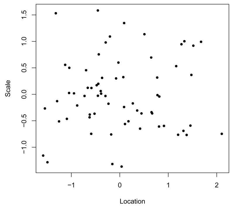
The bivariate scatterplot of the estimated random location (${\tilde{\theta }}_{i1}$ on x-axis) and scale effects (${\tilde{\theta }}_{i2}$ on y-axis) in Figure 3 shows the heterogeneity in both of these subject effects. Note that the scale of both of these are standard normals, and each dot represents the model estimates for a given subject. The non-significance of the location random effect on the WS variance (${\widehat{\tau }}_l$ = 0.213, p = 0.143) that was obtained in the analysis is borne out in the plot, as there is a minimal positive relationship between these two subject-level estimates.

Figure 3.

Bivariate scatter plot of estimated random location and scale effects.

A few subjects are of note in Figure 3, and the data for these subjects are listed in Table 2. First, note the two subjects in the bottom left corner of the plot; these are subjects (ids 117 and 347) with small location and scale effects. These subjects seem to be good responders (i.e., follow a decreasing linear trend across time) with moderate to mild depression values. Conversely, subject 345, who is towards the bottom right corner of the plot, has a large location effect with a relatively small scale effect. This subject does follow a decreasing trend, but is somewhat less responsive and with rather high depression values across time. Subject 505 in the upper left corner, has generally moderate to low depression scores, but a rather erratic pattern across time. Finally, the four subjects (ids 607, 322, 328, and 360) in the upper right corner have generally high depression values which are fairly erratic across time. These subjects do not follow a decreasing linear trend across time, and the last three subjects even display increasing depression values across time.

Table 2.

Interesting subjects in terms of location and scale estimates (i.e., ${\tilde{\theta }}_{1i}$ and ${\tilde{\theta }}_{2i}$) from analysis of the Riesby data (−9 represents missing data).

id	${\tilde{\theta }}_{1i}$	${\tilde{\theta }}_{2i}$	hd0	hd1	hd2	hd3	hd4	hd5
117	−1.492	−1.284	19	16	13	12	7	6
347	−1.580	−1.157	18	15	14	10	8	−9
345	2.104	−0.747	29	27	27	22	22	23
505	−1.320	1.532	21	11	18	0	0	4
607	1.517	0.919	30	39	30	27	20	4
322	1.272	0.946	28	21	25	32	34	−9
328	1.676	0.992	22	24	28	26	28	29
360	1.333	1.003	21	28	27	29	28	33

In the R function, default values have been set to PNINT = 0, RNINT = 0, SNINT = 0, CONV = 0.0005, NQ = 11, AQUAD = 1, MAXIT = 200, NCENT = 0, and NCOV = 1. These can be overwritten in the call to the function. For example, to use 15 quadrature points and to standardize all of the covariates, then the following would be used.

R> mixregls.results2 = mixregls.combined(hamdep ~ endog+week+endweek + | endog | endog+week, id=“id”, data=indata, NQ=15, NCENT=1)

4.3. Intensive longitudinal data with random location and scale

Modern data collection procedures, such as ecological momentary assessments (EMA) (Stone and Shiffman 1994; Smyth and Stone 2003), experience sampling (de Vries 1992; Scollon, Kim-Prieto, and Diener 2003), and diary methods (Bolger et al. 2003), have been developed to record the momentary events and experiences of subjects in daily life. These procedures yield relatively large numbers of subjects and observations per subject, and data from these designs are sometimes referred to as intensive longitudinal data (Walls and Schafer 2006). Such designs are in keeping with the “bursts of measurement” approach described by Nesselroade and McCollam (2000), who called for such an approach in order to assess intra-individual variability. As noted by Nesselroade and McCollam (2000), such bursts of measurement increase the research burden in several ways; however, they are necessary for studying intra-individual variation and to explain why subjects differ in variability rather than solely in mean level (Bolger et al. 2003). As we have described in a series of articles (Hedeker et al. 2008; Hedeker, Demirtas, and Mermelstein 2009; Hedeker, Mermelstein, and Demirtas 2012), mixed-effects location scale analysis of such EMA data is particularly useful.

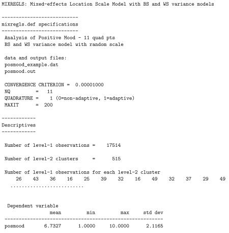
Data for the analyses reported here come from a longitudinal, natural history study of adolescent smoking (Mermelstein, Hedeker, Flay, and Shiffman 2002). Students included in the study were either in 8th or 10th grade at baseline, and self-reported on a screening questionnaire 6-8 weeks prior to baseline that they either had never smoked, but indicated a probability of future smoking, or had smoked in the past 90 days, but had not smoked more than 100 cigarettes in their lifetime. Adolescents carried hand held computers with them at all times during a seven consecutive day data collection period and were trained to both respond to random prompts from the computers and to event record (initiate a data collection interview) smoking episodes. For the analyses reported, we treated the responses obtained from the random prompts. In all, there were 17,514 random prompts obtained from 515 students with an approximate average of 34 prompts per student (range = 3 to 58).

The dependent variable considered is a measure of the subject’s positive mood (posmood) at each random prompt. This measure consists of the average of several individual mood items that were identified via factor analysis. Each item was rated from 1 to 10 with higher values indicating higher levels of positive mood. Over all prompts, and ignoring the clustering of the data, the marginal mean of posmood was 6.733 (sd=2.117). Of interest is the degree of heterogeneity in this mood measure in terms of both WS and BS variation. As covariates, we will examine genderf, which is a subject (level-2) covariate coded 0 for males and 1 for females, and alone, which is a time-varying (level-1) covariate coded 0 if the subject was alone or 1 if with others. Both covariates will be included in all submodels.

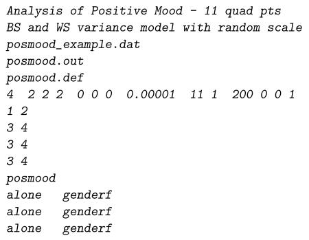
The dataset, named posmood_example.dat, contains four variable fields: id (field 1), posmood (field 2), alone (field 3), and genderf (field 4). The field number is used to identify these variables in the mixregls.def file for the model, which is listed below.

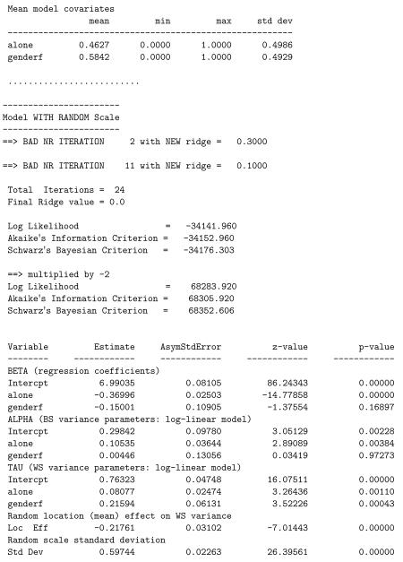
Unlike the Riesby dataset, there are no missing values coded in this dataset, so MISS is set to zero. Other options that are specified in this mixregls.def file: a convergence criterion of 0.00001, 11-point adaptive quadrature, a maximum number of iterations set at 200, and a linear effect of the random location on (log of) the WS variance.

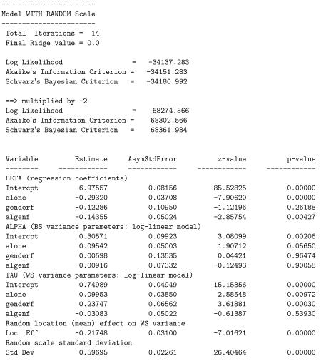
The results for the model are written to the file posmood.out; a partial listing (descriptives and results from the final model stage) is below. Likelihood ratio tests yield: ${\chi }_2^2$ = 70416.708 – 70335.768 = 80.94 comparing stages 1 and 2, and ${\chi }_2^2$ = 70335.768 – 68283.920 = 2051.848 comparing stages 2 and 3. Thus, Model 3 clearly fits better than Model 2, indicating a significant linear effect of the random location effect on the WS variance and subject differences of scale. Notice, that there were two instances of a “BAD NR ITERATION,” which occurred because the likelihood did not increase for the second and eleventh Newton-Raphson (NR) iterations. At those points, the ridge was increased to aid in the computational solution. It is not unusual for there to be a few “bad” iterations, however more than a few would suggest computational problems with the solution. Interpreting the final model stage, we see a significant negative effect of being alone on mean levels of positive mood, namely, subjects have worse mood when alone. Additionally, being alone increases the BS variance, and so subjects are more heterogeneous in mood when they are alone. The gender effect on the mean level and the BS variance are not seen to be significant. However, females exhibit greater WS positive mood variance, as does being alone. The mood responses of a subject are more heterogeneous and less stable for females, relative to males. Also, for a given subject, their mood responses are more varied when they are alone, relative to when they are with others.

Expressing the variance estimates in terms of intraclass correlation

Based on the current analysis, the (log-linear) model for the BS variance is given by

$${\sigma }_{v_{\mathit{ij}}}^2=\exp ({\alpha }_0+{\alpha }_1{\text{alone}}_{\mathit{ij}}+{\alpha }_2{\text{genderf}}_i).$$ (15)

Thus, we can estimate the BS variance for the four cells of the crossing of the two indicator variables (male/female by alone/not alone) as:

$$\begin{array}{cc}\hfill \text{male},\text{not}\text{alone}:{\widehat{\sigma }}_v^2=& \exp \left(0.2984\right)=1.348,\hfill \\ \hfill \text{male},\text{alone}:{\widehat{\sigma }}_v^2=& \exp (0.2984+0.10535)=1.497,\hfill \\ \hfill \text{female},\text{not}\text{alone}:{\widehat{\sigma }}_v^2=& \exp (0.2984+0.00446)=1.354,\hfill \\ \hfill \text{female},\text{alone}:{\widehat{\sigma }}_v^2=& \exp (0.2984+0.10535+0.00446)=1.504.\hfill \end{array}$$

These estimates show the increased heterogeneity across subjects for both gender groups when they are alone, relative to when they are with others. In terms of the WS variance, the (log-linear) model is:

$${\sigma }_{{∊}_{\mathit{ij}}}^2=\exp ({\tau }_0+{\tau }_1{\text{alone}}_i+{\tau }_2{\text{genderf}}_i+0.5({\tau }_l^2+{\sigma }_{\omega }^2\left)\right).$$ (16)

The form for the latter two terms are based on the expectation of the log-normally distributed θ_1i and θ_2i (see Skrondal and Rabe-Hesketh (2004) page 124). For this analysis, $0.5({\widehat{\tau }}_l^2+{\widehat{\sigma }}_{\omega }^2)=0.5({(-0.2176)}^2+{\left(0.5974\right)}^2)=0.2021$. Using this estimate, the WS variance for each of the four cells (male/female by alone/not alone) is estimated as:

$$\begin{array}{cc}\hfill \text{male},\text{not}\text{alone}:{\widehat{\sigma }}_{∊}^2=& \exp (0.7632+0.2021)=2.626,\hfill \\ \hfill \text{male},\text{alone}:{\widehat{\sigma }}_{∊}^2=& \exp (0.7632+0.0808+0.2021)=2.847,\hfill \\ \hfill \text{female},\text{not}\text{alone}:{\widehat{\sigma }}_{∊}^2=& \exp (0.7632+02159+0.2021)=3.259,\hfill \\ \hfill \text{female},\text{alone}:{\widehat{\sigma }}_{∊}^2=& \exp (0.7632+0.0808+0.2159+0.2021)=3.533.\hfill \end{array}$$

Thus, there is more WS variance for females, relative to males, and also when alone, relative to not alone. The intraclass correlation, $r={\sigma }_v^2∕({\sigma }_v^2+{\sigma }_{∊}^2)$, can be estimated as:

$$\begin{array}{cc}\hfill \text{male},\text{not}\text{alone}:\widehat{r}=& 1.348∕(1.348+2.626)=0.339,\hfill \\ \hfill \text{male},\text{alone}:\widehat{r}=& 1.497∕(1.497+2.847)=0.345,\hfill \\ \hfill \text{female},\text{not}\text{alone}:\widehat{r}=& 1.354∕(1.354+3.259)=0.294,\hfill \\ \hfill \text{female},\text{alone}:\widehat{r}=& 1.504∕(1.504+3.533)=0.299.\hfill \end{array}$$

As can be seen, the data are more correlated (i.e., less heterogeneous) within males, than females, and not too different when alone versus not alone. The latter result occurs because being alone increases both the WS and BS variances. However, in terms of gender, the intraclass correlation estimates vary because while the BS variance is very similar between males and females, the WS variance (which forms part of the denominator in the intraclass correlation equation) is increased for females, relative to males.

4.4. Running MIXREGLS from SAS

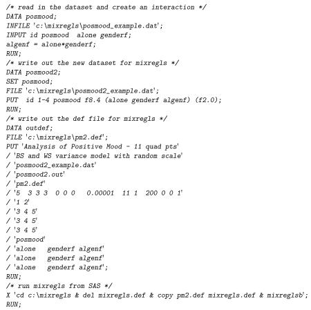
For the current dataset, one might be interested in examining, say, the interaction between genderf and alone on posmood. MIXREGLS does not have data management capabilities, but it is easy to use SAS, for example, to create this interaction and run MIXREGLS. For this, the SAS code, listed below, reads in posmood_example.dat, creates the interaction of genderf and alone, writes out a new dataset posmood2_example.dat, writes out a new definition file pm2.def, and issues the command prompts to run MIXREGLS using the new definition file. This is done by the X statement in SAS, which allows Windows commands to be executed. Notice that the multiple commands are in quotes and separated by the & symbol. In running this program in SAS, a command prompt screen will open up as MIXREGLS is running.

Below is a listing of the results from the final model stage for this analysis that includes the interaction of alone by genderf. The likelihood ratio test comparing this model to the previous one yields ${\chi }_3^2$ = 68283.920 − 68274.566 = 9.354 which is statistically significant at the 0.025 level. Thus, there is evidence of significant interaction. Looking at the interaction effects in the three submodels, we see that the interaction is significant only in the mean submodel. The nature of this interaction, in terms of the mean, is that there is no significant gender effect when subjects are not alone, but a highly significant gender difference, with females being lower than males, when subjects are alone. Or, another way of expressing it is that while both males and females are lower on positive mood when they are alone, relative to when they are not alone, this difference is significantly greater for females than males.

4.5. Quadratic effect of the random location effect on WS variance

As previously described, a quadratic relationship between a subject’s mean and the log of their WS variance can be specifed through use of the NCOV option on line 6 (last option on this line) of the mixregls.def file. Specifically, this option allows either:

$$\mathrm{NCOV}=0:{\sigma }_{{∊}_{\mathit{ij}}}^2=\exp (w_{\mathit{ij}}^{⊺}\tau +{\sigma }_{\omega }{\theta }_{2i}),$$ (17)

$$\mathrm{NCOV}=1:{\sigma }_{{∊}_{\mathit{ij}}}^2=\exp (w_{\mathit{ij}}^{⊺}\tau +{\tau }_l{\theta }_{1i}+{\sigma }_{\omega }{\theta }_{2i}),$$ (18)

$$\mathrm{NCOV}=2:{\sigma }_{{∊}_{\mathit{ij}}}^2=\exp (w_{\mathit{ij}}^{⊺}\tau +{\tau }_l{\theta }_{1i}+{\tau }_q{\theta }_{1i}^2+{\sigma }_{\omega }{\theta }_{2i}).$$ (19)

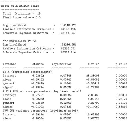
Thus far, all of our examples have considered NCOV=1 to allow for a linear association. By changing this value from 1 to 2, we can investigate whether the linear association is sufficient, relative to a quadratic relationship. Using the current example, this one change to the mixregls.def file produces the results listed below.

A likelihood ratio test yields ${\chi }_1^2$ = 68274.566 − 68236.251 = 38.32 for the null hypothesis H₀: τ_q = 0, clearly rejecting the null. Thus, the current model with the linear and quadratic effects fits the data significantly better than the previous model with only the linear effect. As can be seen, both linear and quadratic location effects are negative and significant. This suggests that subjects with higher location effects (more positive affect) exhibit less WS variation in more than a linear manner (on the log scale). As previously mentioned, this could be due to a ceiling effect of measurement in that subjects with high mean levels of positive affect (towards the maximum of 10) must exhibit low variation in their scores. In terms of the other model estimates, most are very similar to those obtained previously in the model with only the linear location effect, and none of the conclusions change appreciably.

5. Discussion

This article has described the program MIXREGLS which can be used to estimate the parameters of a mixed-effects location scale model (Hedeker et al. 2008). This extended mixed model augments the usual mean model with sub-models of the BS and WS variances. Covariates can be included in each of these sub-models. Relative to the standard mixed model, this augmented approach can be useful to identify predictors of both WS and BS variation, and to test hypotheses about these variances. Also, by including a random subject effect on the WS variance, this model can examine the degree to which subjects are heterogeneous in terms of their variation on the outcome variable, over and above the covariate effects. The random scale effects are further allowed to be associated with the usual random location effects, and this association can either be of a linear or quadratic form (in the log-linear model of the WS variance). Modern data collection procedures, such as EMA and/or real-time data captures, are increasingly used in many research areas. These approaches often provide a fair amount of both WS and BS data, and so allow the opportunity for modeling of both WS and BS variances as a function of covariates.

MIXREGLS is appropriate for continuous outcomes that are (conditionally) normally distributed. For ordinal outcomes, we have also described a mixed-effects location scale model (Hedeker et al. 2009). In the ordinal approach, we extend the mixed-effects logistic regression model of Hedeker and Gibbons (1994) by including the log-linear modeling of BS and WS variance, as well as the random scale effect. SAS NLMIXED can be used to estimate the parameters of the ordinal location-scale model, and Hedeker et al. (2009) includes sample syntax, however, as in the continuous case, it is rather slow to converge and can be sensitive to the specification of starting values. Thus, in future work we hope to develop an ordinal version of MIXREGLS as well.

Another limitation is that MIXREGLS only includes a random intercept as the location effect. For longitudinal data, a more general model with multiple random location effects is often used (Hedeker and Gibbons 2006), for example, to allow subjects to vary in terms of the model intercepts and time-trends. Also, MIXREGLS only allows estimation of a two-level model (i.e., repeated observations within subjects, or subjects within clusters), however in some cases a more extended hierarchical model is necessary. For example, for the EMA dataset one might consider a three-level model in which observations (level 1) are nested within days (level 2) within subjects (level 3). In a recent paper, Li and Hedeker (2012) proposed such a three-level model for EMA data, including development of a recursive conditional likelihood approach using SAS NLMIXED to estimate the model parameters. Future work on MIXREGLS will hopefully include some of these extensions of the model.

A. Estimation details

In terms of estimation, the model can be written as:

$${∊}_{\mathit{ij}}=y_{\mathit{ij}}-\left(x_{\mathit{ij}}^{⊺}\beta +{\sigma }_{vi}{\theta }_{1i}\right),$$ (20)

and

$${\sigma }_{v_{\mathit{ij}}}^2=\exp \left(u_{\mathit{ij}}^{⊺}\alpha \right),$$ (21)

which allows the model to be expressed as:

$${∊}_{\mathit{ij}}=y_{\mathit{ij}}-\left(x_{\mathit{ij}}^{⊺}\beta +\sqrt{\exp \left(u_{\mathit{ij}}^{⊺}\alpha \right)}{\theta }_{1i}\right),$$ (22)

where the error variance is given by:

$${\sigma }_{{∊}_{\mathit{ij}}}^2=\exp (w_{\mathit{ij}}^{⊺}\tau +{\tau }_l{\theta }_{1i}+{\tau }_q{\theta }_{1i}^2+{\sigma }_{\omega }{\theta }_{2i})=\exp (w_{\mathit{ij}}^{⊺}\tau +s_i^{⊺}{\theta }_i^{\ast }),$$ (23)

with $s^{⊺}=\left[\begin{array}{ccc}\hfill {\tau }_l\hfill & \hfill {\tau }_q\hfill & \hfill {\sigma }_{\omega }\hfill \end{array}\right]$ and ${\theta }_i^{\ast }={\left[\begin{array}{ccc}\hfill {\theta }_{1i}\hfill & \hfill {\theta }_{1i}^2\hfill & \hfill {\theta }_{2i}\hfill \end{array}\right]}^{⊺}$. Under the conditional independence assumption, in which the responses within a subject are independent conditional on the random subject effects, ${\theta }_i={\left[\begin{array}{cc}\hfill {\theta }_{1i}\hfill & \hfill {\theta }_{2i}\hfill \end{array}\right]}^{⊺}$, the conditional log-likelihood for a given subject is

$$\ln l({∊}_i\mid \theta )=-\frac{1}{2}\sum ^{n_i}{f}_{\mathit{ij}},$$ (24)

with

$$f_{\mathit{ij}}=\ln 2\pi {\sigma }_{{∊}_{\mathit{ij}}}^2+{∊}_{\mathit{ij}}^2∕{\sigma }_{{∊}_{\mathit{ij}}}^2.$$ (25)

The marginal likelihood is obtained by integrating over the standardized random effects:

$$h\left({∊}_i\right)={\int }_{\theta }l({∊}_i\mid \theta )g\left(\theta \right)d\theta ,$$ (26)

where g(θ) is a standard bivariate normal density. The marginal log-likelihood from the sample of N subjects is then obtained as $\ln L={\sum }_i^N\ln h\left({∊}_i\right)$. Maximizing this log-likelihood yields maximum likelihood (ML) estimates, which are sometimes referred to as maximum marginal likelihood estimates (Bock 1989) because integrating the joint likelihood of random effects and responses over the distribution of random effects translates to marginalization of the data distribution.

MIXREGLS maximizes this log-likelihood using a Newton-Raphson algorithm. For this, both the first and second derivatives of the log-likelihood, with respect to the model parameters, must be derived. To simplify the notation, denote h_i = h(∊_i) and l_i = l(∊_i|θ). Also, let η represent an arbitrary parameter vector (i.e., β, α, τ, or s). Then,

$$\frac{\partial \ln L}{\partial \eta }=\sum _i^N{h}_i^{-1}{\int }_{\theta }\frac{\partial \ln l_i}{\partial \eta }{l}_{i}g\left(\theta \right)d\theta ,$$ (27)

and

$$\frac{\partial \ln l_i}{\partial \eta }=-\frac{1}{2}\sum ^{n_i}\frac{\partial f_{\mathit{ij}}}{\partial \eta }.$$ (28)

For the first derivatives, we obtain:

$$\frac{\partial f_{\mathit{ij}}}{\partial \beta }=-2{\sigma }_{{∊}_{\mathit{ij}}}^{-2}{∊}_{\mathit{ij}}{\mathit{x}}_{\mathit{ij}},$$ (29)

$$\frac{\partial f_{\mathit{ij}}}{\partial \alpha }=-{\sigma }_{{∊}_{\mathit{ij}}}^{-2}{∊}_{\mathit{ij}}{\theta }_{1i}{\sigma }_{v_{\mathit{ij}}}{\mathit{u}}_{\mathit{ij}},$$ (30)

$$\frac{\partial f_{\mathit{ij}}}{\partial \tau }=\left[1-{\sigma }_{{∊}_{\mathit{ij}}}^{-2}{∊}_{\mathit{ij}}^2\right]{\mathit{w}}_{\mathit{ij}},$$ (31)

$$\frac{\partial f_{\mathit{ij}}}{\partial \mathit{s}}=\left[1-{\sigma }_{{∊}_{\mathit{ij}}}^{-2}{∊}_{\mathit{ij}}^2\right]{\theta }_i^{\ast }.$$ (32)

To derive the matrix of second derivatives, denote

$$\frac{\partial \ln L}{\partial \eta }=\sum _{i=1}^N{h}_i^{-1}{\mathit{d}}_i,$$ (33)

where

$${\mathit{d}}_i={\int }_{\theta }\frac{\partial \ln l_i}{\partial \eta }{l}_{i}g\left(\theta \right)d\theta .$$ (34)

Notice that d_i is equal to ∂h_i/∂η, so that

$$\frac{{\partial }^2\ln L}{\partial \eta \partial {\eta }^{⊺}}=\sum _{i=1}^N{h}_i^{-2}\left[h_i\frac{\partial {\mathit{d}}_i}{\partial \eta }-{\mathit{d}}_i\frac{\partial h_i}{\partial {\eta }^{⊺}}\right]=\sum _{i=1}^N{h}_i^{-2}\left[h_i\frac{\partial {\mathit{d}}_i}{\partial \eta }-{\mathit{d}}_i{\mathit{d}}_i^{⊺}\right],$$ (35)

where

$$\frac{\partial {\mathit{d}}_i}{\partial \eta }={\int }_{\theta }\left[\left(\frac{\partial \ln l_i}{\partial \eta }\right){\left(\frac{\partial \ln l_i}{\partial \eta }\right)}^{⊺}+\frac{{\partial }^2\ln l_i}{\partial \eta \partial {\eta }^{⊺}}\right]l_{i}g\left(\theta \right)d\theta .$$ (36)

Thus, we need to derive the second derivatives with respect to ln l_i. These are obtained as:

$$\frac{{\partial }^2\ln l_i}{\partial \beta \partial {\beta }^{⊺}}=-\sum ^{n_i}{\sigma }_{{∊}_{\mathit{ij}}}^{-2}{\mathit{x}}_{\mathit{ij}}{\mathit{x}}_{\mathit{ij}}^{⊺},$$ (37)

$$\frac{{\partial }^2\ln l_i}{\partial \alpha \partial {\alpha }^{⊺}}=-\frac{1}{4}\sum ^{n_i}{\sigma }_{{∊}_{\mathit{ij}}}^{-2}{\theta }_{1i}{\sigma }_{v_{\mathit{ij}}}({\theta }_{1i}{\sigma }_{v_{\mathit{ij}}}-{∊}_{\mathit{ij}}){\mathit{u}}_{\mathit{ij}}{\mathit{u}}_{\mathit{ij}}^{⊺},$$ (38)

$$\frac{{\partial }^2\ln l_i}{\partial \tau \partial {\tau }^{⊺}}=-\frac{1}{2}\sum ^{n_i}{\sigma }_{{∊}_{\mathit{ij}}}^{-2}{∊}_{\mathit{ij}}^2{\mathit{w}}_{\mathit{ij}}{\mathit{w}}_{\mathit{ij}}^{⊺},$$ (39)

$$\frac{{\partial }^2\ln l_i}{\partial \tau \partial {\tau }^{⊺}}=-\frac{1}{2}\sum ^{n_i}{\sigma }_{{∊}_{\mathit{ij}}}^{-2}{∊}_{\mathit{ij}}^2{\theta }_i^{\ast }{\left({\theta }_i^{\ast }\right)}^{⊺}.$$ (40)

The above are for the diagonal blocks of the second derivative matrix. For the off-diagonal blocks, we obtain

$$\frac{{\partial }^2\ln l_i}{\partial \alpha \partial {\beta }^{⊺}}=-\frac{1}{2}\sum ^{n_i}{\sigma }_{{∊}_{\mathit{ij}}}^{-2}{\theta }_{1i}{\sigma }_{v_{\mathit{ij}}}{\mathit{u}}_{\mathit{ij}}{\mathit{x}}_{\mathit{ij}}^{⊺},$$ (41)

$$\frac{{\partial }^2\ln l_i}{\partial \tau \partial {\beta }^{⊺}}=-\sum ^{n_i}{\sigma }_{{∊}_{\mathit{ij}}}^{-2}{∊}_{\mathit{ij}}{\mathit{w}}_{\mathit{ij}}{\mathit{x}}_{\mathit{ij}}^{⊺},$$ (42)

$$\frac{{\partial }^2\ln l_i}{\partial \tau \partial {\alpha }^{⊺}}=-\frac{1}{2}\sum ^{n_i}{\sigma }_{{∊}_{\mathit{ij}}}^{-2}{\theta }_{1i}{∊}_{\mathit{ij}}{\sigma }_{v_{\mathit{ij}}}{\mathit{w}}_{\mathit{ij}}{\mathit{u}}_{\mathit{ij}}^{⊺},$$ (43)

$$\frac{{\partial }^2\ln l_i}{\partial \mathit{s}\partial {\beta }^{⊺}}=-\sum ^{n_i}{\sigma }_{{∊}_{\mathit{ij}}}^{-2}{∊}_{\mathit{ij}}{\theta }_i^{\ast }{\mathit{x}}_{\mathit{ij}}^{⊺},$$ (44)

$$\frac{{\partial }^2\ln l_i}{\partial \mathit{s}\partial {\alpha }^{⊺}}=-\frac{1}{2}\sum ^{n_i}{\sigma }_{{∊}_{\mathit{ij}}}^{-2}{\theta }_{1i}{∊}_{\mathit{ij}}{\sigma }_{v_{\mathit{ij}}}{\theta }_i^{\ast }{\mathit{u}}_{\mathit{ij}}^{⊺},$$ (45)

$$\frac{{\partial }^2\ln l_i}{\partial \mathit{s}\partial {\tau }^{⊺}}=-\frac{1}{2}\sum ^{n_i}{\sigma }_{{∊}_{\mathit{ij}}}^{-2}{∊}_{\mathit{ij}}^2{\theta }_i^{\ast }{\mathit{w}}_{\mathit{ij}}^{⊺}.$$ (46)

The Newton-Raphson iterative procedure can now be implemented. Specifically, estimates for the entire vector of parameters ζ, on iteration ι are improved by

$${\zeta }_{\iota +1}={\zeta }_{\iota }-{\left[\frac{{\partial }^2\ln L}{\partial {\zeta }_{\iota }\partial {\zeta }_{\iota }^{⊺}}\right]}^{-1}\frac{\partial \ln L}{\partial {\zeta }_{\iota }}.$$ (47)

At each model stage, MIXREGLS continues to iterate until all of the corrections (ζ_ι+1 − ζ_ι) are less, in absolute value, than the convergence criterion CONV specified in the mixregls.def definition file. At convergence, the ML estimates and their accompanying standard errors can be used to construct asymptotic z-statistics by dividing the parameter estimate by its standard error (Wald 1943). The computed z-statistic can then be compared with the standard normal table to test whether the parameter is significantly different from zero. MIXREGLS lists these z- and p-values, in addition to the parameter estimates and their standard errors. Also, the likelihood-ratio (or difference in log-likelihood) χ² test can be used for comparison of nested models, for example, the three sequential models that MIXREGLS fits. For this, the significance of the additional terms in model A over model B is determined by comparing −2(ln L_B − ln L_A) to a table of the χ² distribution with degrees of freedom equal to the number of additional parameters in model A. To facillitate this, MIXREGLS lists the deviance (−2 ln L) of each of the sequential models that it estimates.

A.1. Numerical quadrature

In order to solve the above likelihood equations, numerical integration on the random effect θ space must be performed. For this, Gauss-Hermite quadrature can be used to approximate the above integrals to any practical degree of accuracy (Stroud and Sechrest 1966). In Gauss-Hermite quadrature, the integration is approximated by a summation on a specified number of quadrature points NQ for each dimension of the integration; thus, for the bivariate θ space, the summation goes over NQ² points. MIXREGLS allows for both ordinary quadrature, in which the same points are used for all subjects, or adaptive quadrature (Bock and Shilling 1997; Rabe-Hesketh, Skrondal, and Pickles 2002), in which the points are adapted to the location and dispersion for each subject at each iteration. The benefit of adaptive quadrature is that it usually requires a smaller number of quadrature points to achieve convergence.

At each iteration, and for each subject, the solution goes over the NQ² quadrature points, with summation replacing the integration over the random-effect distribution. The conditional likelihoods l_i are obtained substituting the random-effect vector θ by the current 2-dimensional vector of quadrature points B_q. The marginal density for each level-2 unit is then approximated as

$$h_i\approx \sum _q^{{\mathrm{NQ}}^2}{l}_i({∊}_i\mid {\mathit{B}}_q)A\left({\mathit{B}}_q\right).$$ (48)

At each iteration, computation of the first derivatives and second derivative matrix then proceeds summing over subjects and quadrature points. In the summation over the NQ² quadrature points, the θ random-effect vector is substituted by the current vector of quadrature points B_q, and the evaluation of the density g(θ) is substituted by the current quadrature weight A(B_q), which is obtained as the product of the quadrature weights from the two dimensions of the integral. Following the summation over subjects and quadrature points, parameters are corrected according to the Newton-Raphson algorithm, and the entire procedure is repeated until convergence.

A.2. Estimation of random effects

As was illustrated in the first example, it can be of interest to examine the estimates of the random effects θ_i within the sample. A reasonable choice for this is the expected “a posteriori” (EAP) or empirical Bayes estimator ${\stackrel{‒}{\theta }}_i$ (Bock and Aitken 1981). For the univariate case, this estimator ${\stackrel{‒}{\theta }}_i$ is given by:

$${\stackrel{‒}{\theta }}_i=E({\theta }_i\mid {∊}_i)=\frac{1}{h\left({∊}_i\right)}{\int }_{\theta }{\theta }_{i}l({∊}_i\mid {\theta }_i)g\left(\theta \right)d\theta .$$ (49)

The variance of this estimator is obtained similarly as:

$$V({\stackrel{‒}{\theta }}_i\mid {∊}_i)=\frac{1}{h\left({∊}_i\right)}{\int }_{\theta }{({\theta }_i-{\stackrel{‒}{\theta }}_i)}^2{l}_{i}g\left(\theta \right)d\theta .$$ (50)

Upon convergence of each stage, MIXREGLS estimates these quantities using one additional round of quadrature. As mentioned in the first example, these estimates are written out to the file mixregls.re2. They may then be used, for example, to evaluate the location and scale estimates for particular subjects.

A.3. Standardized residuals

For each of the three model stages, the standardized residuals are obtained as:

$${\widehat{\xi }}_{\mathit{ij}}=\frac{y_{\mathit{ij}}-\left({\mathit{x}}_{\mathit{ij}}^{⊺}\widehat{\beta }+\sqrt{\exp \left({\mathit{u}}_{\mathit{ij}}^{⊺}\widehat{\alpha }\right)}{\tilde{\theta }}_{1i}\right)}{{\widehat{\sigma }}_{{∊}_{\mathit{ij}}}}.$$ (51)

Note that the denominator, which is the WS standard deviation, varies for the three model stages. For stages 1 and 2, it equals $\sqrt{\exp \left(w_{ij}^{⊺}\widehat{\tau }\right)}$, while for stage 3 it varies depending on the NCOV specification:

$$\mathrm{NCOV}=0:{\widehat{\sigma }}_{{∊}_{\mathit{ij}}}=\sqrt{\exp ({\mathit{w}}_{\mathit{ij}}^{⊺}\widehat{\tau }+{\widehat{\sigma }}_{\omega }{\tilde{\theta }}_{2i})}$$ (52)

$$\mathrm{NCOV}=1:{\widehat{\sigma }}_{{∊}_{\mathit{ij}}}=\sqrt{\exp ({\mathit{w}}_{\mathit{ij}}^{⊺}\widehat{\tau }+{\widehat{\tau }}_l{\tilde{\theta }}_{1i}+{\widehat{\sigma }}_{\omega }{\tilde{\theta }}_{2i})}$$ (53)

$$\mathrm{NCOV}=2:{\widehat{\sigma }}_{{∊}_{\mathit{ij}}}=\sqrt{\exp ({\mathit{w}}_{\mathit{ij}}^{⊺}\widehat{\tau }+{\widehat{\tau }}_l{\tilde{\theta }}_{1i}+{\widehat{\tau }}_q{\left({\tilde{\theta }}_{1i}\right)}^2+{\widehat{\sigma }}_{\omega }{\tilde{\theta }}_{2i})}$$ (54)

The residuals from all model stages are output to the file mixregls.re1; these can be plotted, for example, to assess the assumption of normality of the model errors.

References

- Aitkin M. Modelling Variance Heterogeneity in Normal Regression Using GLIM. Applied Statistics. 1987;36:332–339. [Google Scholar]
- Bock RD. Multivariate Statistical Methods in Behavioral Research. McGraw-Hill; New York: 1975. [Google Scholar]
- Bock RD. Measurement of Human Variation: A Two Stage Model. In: Bock RD, editor. Multilevel Analysis of Educational Data. Academic Press; New York: 1989. [Google Scholar]
- Bock RD, Aitken M. Marginal Maximum Likelihood Estimation of Item Parameters: An Application of the EM Algorithm. Psychometrika. 1981;46:443–459. [Google Scholar]
- Bock RD, Shilling S. High-Dimensional Full-Information Item Factor Analysis. In: Berkane M, editor. Latent Variable Modeling and Applications to Causality. Springer-Verlag; New York: 1997. pp. 163–176. [Google Scholar]
- Bolger N, Davis A, Rafaeli E. Diary Methods: Capturing Life as it is Lived. Annual Review of Psychology. 2003;54:579–616. doi: 10.1146/annurev.psych.54.101601.145030. [DOI] [PubMed] [Google Scholar]
- de Vries M. The Experience of Psychopathology: Investigating Mental Disorders in Their Natural Settings. Cambridge University Press; New York: 1992. [Google Scholar]
- Fleeson W. Moving Personality Beyond the Person-Situation Debate. Current Directions in Psychological Science. 2004;13:83–87. [Google Scholar]
- Fowler K, Whitlock MC. The Distribution of Phenotypic Variance with Inbreeding. Evolution. 1999;53:1143–1156. doi: 10.1111/j.1558-5646.1999.tb04528.x. [DOI] [PubMed] [Google Scholar]
- Goldstein H. Multilevel Statistical Models. 4 edition John Wiley & Sons; Chichester, UK: 2011. [Google Scholar]
- Harvey AC. Estimating Regression Models with Multiplicative Heteroscedasticity. Econometrica. 1976;44:461–465. [Google Scholar]
- Hedeker D, Demirtas H, Mermelstein RJ. A Mixed Ordinal Location Scale Model for Analysis of Ecological Momentary Assessment (EMA) Data. Statistics and Its Interface. 2009;2:391–402. doi: 10.4310/sii.2009.v2.n4.a1. [DOI] [PMC free article] [PubMed] [Google Scholar]
- Hedeker D, Gibbons RD. A Random-Effects Ordinal Regression Model for Multilevel Analysis. Biometrics. 1994:933–944. [PubMed] [Google Scholar]
- Hedeker D, Gibbons RD. MIXREG: A Computer Program for Mixed-Effects Regression Analysis with Autocorrelated Errors. Computer Methods and Programs in Biomedicine. 1996;49:229–252. doi: 10.1016/0169-2607(96)01723-3. [DOI] [PubMed] [Google Scholar]
- Hedeker D, Gibbons RD. Longitudinal Data Analysis. John Wiley & Sons; Hoboken, NJ: 2006. [Google Scholar]
- Hedeker D, Mermelstein RJ, Demirtas H. An Application of a Mixed-Effects Location Scale Model for Analysis of Ecological Momentary Assessment (EMA) Data. Biometrics. 2008;64:627–634. doi: 10.1111/j.1541-0420.2007.00924.x. [DOI] [PMC free article] [PubMed] [Google Scholar]
- Hedeker D, Mermelstein RJ, Demirtas H. Modeling Between- and Within-Subject Variance in Ecological Momentary Assessment (EMA) Data Using Mixed-Effects Location Scale Models. Statistics in Medicine. 2012;31:3328–3336. doi: 10.1002/sim.5338. [DOI] [PMC free article] [PubMed] [Google Scholar]
- Hertzog C, Nesselroade JR. Assessing Psychological Change in Adulthood: An Overview of Methodological Issues. Psychology and Aging. 2003;18:639–657. doi: 10.1037/0882-7974.18.4.639. [DOI] [PubMed] [Google Scholar]
- Lemmon DR, Schafer JL. Developing Statistical Software in Fortran 95. Springer-Verlag; New York: 2005. [Google Scholar]
- Leonard T. A Bayesian Approach to the Linear Model with Unequal Variances. Technometrics. 1975;17:95–102. [Google Scholar]
- Li X, Hedeker D. A Three-Level Mixed-Effects Location Scale Model with an Application to Ecological Momentary Assessment (EMA) Data. Statistics in Medicine. 2012;31:3192–3210. doi: 10.1002/sim.5393. [DOI] [PMC free article] [PubMed] [Google Scholar]
- Little RJA, Rubin DB. Statistical Analysis with Missing Data. 2 edition John Wiley & Sons; Hoboken, NJ: 2002. [Google Scholar]
- Martin M, Hofer SM. Intraindividual Variability, Change, and Aging: Conceptual and Analytical Issues. Gerontology. 2004;50:7–11. doi: 10.1159/000074382. [DOI] [PubMed] [Google Scholar]
- Mermelstein R, Hedeker D, Flay B, Shiffman S. Situational Versus Intra-Individual Contributions to Adolescents’ Subjective Mood Experience of Smoking; Annual Meeting for the Society for Research on Nicotine and Tobacco; Savannah, GA. 2002. [Google Scholar]
- Nesselroade JR. Intraindividual Variability and Short-Term Change. Gerontology. 2004;50:44–47. doi: 10.1159/000074389. [DOI] [PubMed] [Google Scholar]
- Nesselroade JR, McCollam KMS. Putting the Process in Developmental Processes. International Journal of Behavioral Development. 2000;24:295–300. [Google Scholar]
- Rabe-Hesketh S, Skrondal A, Pickles A. Reliable Estimation of Generalized Linear Mixed Models using Adaptive Quadrature. The Stata Journal. 2002;2:1–21. [Google Scholar]
- Raudenbush SW, Bryk AS. Hierarchical Linear Models. 2 edition Sage Publications; Thousand Oaks, CA: 2002. [Google Scholar]
- Reisby N, Gram LF, Bech P, Nagy A, Petersen GO, Ortmann J, Ibsen I, Dencker SJ, Jacobsen O, Krautwald O, Sondergaard I, Christiansen J. Imipramine: Clinical Effects and Pharmacokinetic Variability. Psychopharmacology. 1977;54:263–272. doi: 10.1007/BF00426574. [DOI] [PubMed] [Google Scholar]
- Renò R, Rizza R. Is Volatility Lognormal? Evidence from Italian Futures. Physica A: Statistical Mechanics and its Applications. 2003;322:620–628. [Google Scholar]
- Scollon CN, Kim-Prieto C, Diener E. Experience Sampling: Promises and Pitfalls, Strengths and Weaknesses. Journal of Happiness Studies. 2003;4:5–34. [Google Scholar]
- Shenk TM, White GC, Burnhamb KP. Sampling-Variance Effects on Detecting Density Dependence from Temporal Trends in Natural Populations. Ecological Monographs. 1998;68:445–463. [Google Scholar]
- Skrondal A, Rabe-Hesketh S. Generalized Latent Variable Modeling. Chapman & Hall/CRC Press; Boca Raton, FL: 2004. [Google Scholar]
- Smyth JM, Stone AA. Ecological Momentary Assessment Research in Behavioral Medicine. Journal of Happiness Studies. 2003;4:35–52. [Google Scholar]
- Stone A, Shiffman S. Ecological Momentary Assessment (EMA) in Behavioral Medicine. Annals of Behavioral Medicine. 1994;16:199–202. [Google Scholar]
- Stroud AH, Sechrest D. Gaussian Quadrature Formulas. Prentice Hall; Englewood Cliffs, NJ: 1966. [Google Scholar]
- Vasseur H. Prediction of Tropospheric Scintillation on Satellite Links from Radiosonde Data. IEEE Transactions on Antennas and Propagation. 1999;47:293–301. [Google Scholar]
- Verbeke G, Molenberghs G. Linear Mixed Models for Longitudinal Data. Springer-Verlag; New York: 2000. [Google Scholar]
- Wald A. Tests of Statistical Hypotheses Concerning Several Parameters When the Number of Observations is Large. Transactions of the American Mathematical Society. 1943;54:426–482. [Google Scholar]
- Walls TA, Schafer JL. Models for Intensive Longitudinal Data. Oxford University Press; New York: 2006. [Google Scholar]
- Zeileis A, Croissant Y. Extended Model Formulas in R: Multiple Parts and Multiple Responses. Journal of Statistical Software. 2010;34(XYZ):1–12. URL http://www.jstatsoft.org/v34/iXYZ/ [Google Scholar]