Reference region approaches in PET: a comparative study on multiple radioligands

Abstract

Reference region (RR) approaches (RRAs) for positron emission tomography (PET) brain studies aim to obtain full quantification without arterial input function (IF) sampling, an invasive and costly procedure. Although they need a reliable RR and are only able to estimate the nondisplaceable binding potential (BP_ND), RRAs are widely used. If quantitatively reliable, then RRAs can greatly benefit PET investigations, but their suitability can vary widely from radioligand to radioligand. This study compares estimates of BP_ND both using IF data and several common RRAs on an extensive data set for each of several radioligands. In addition, two new methods, likelihood estimation in graphical analysis with RR and a bootstrapping algorithm for estimating precision, are presented here for the first time. Although many factors contribute to the performance of each RRA, our results suggest that the kinetics in the RR have a role. In particular, RRAs tend to be good when (1) the RR distribution volume is high; (2) the transfer rate constant from plasma to free compartment in the RR is high; and (3) the transfer rate constant from free to plasma compartment in the RR is low.

Introduction

Positron emission tomography (PET), a nuclear imaging technology that uses radioactively labeled molecules (i.e., radioligands) for quantifying and visualizing in vivo biologic processes, represents an invaluable tool for assessing the pathology of several brain disorders. Full quantification in PET, particularly with new radioligands, involves determining the free (unbound to plasma proteins) radioligand concentration in the arterial plasma—the input function (IF)—to quantify the tissue radioligand uptake and separate tissue binding from delivery and blood flow effects. Input function is typically obtained by inserting a catheter into the subject's radial artery, collecting blood samples at several times during the scan, and measuring the radioligand concentration. If the radioligand metabolizes in the body, then several of these samples also undergo metabolite analysis to determine the fraction of unmetabolized parent compound to correct the IF accordingly (i.e., metabolite-corrected IF, cIF). This procedure is invasive and costly. It tends to deter subjects' participation and requires highly specialized medical staff and equipment to perform blood analysis.

For all these reasons, much effort has been devoted to obtaining fully quantitative PET imaging without cIF, including the development of reference region (RR) approaches (RRAs), such as full (FRTM)^{1, 2, 3} and simplified reference tissue model (SRTM),⁴ Logan RR,⁵ and multilinear reference tissue models (MRTMs).^{6, 7} Reference region approaches do not require arterial sampling by forming an inferred relationship between regions, based on the fact that such regions share the cIF, and assuming that the radioligand nondisplaceable volume of distribution (V_ND), ideally the volume of distribution (V_T) in an RR devoid of specific binding, is constant throughout the brain.

In order for the approach to be valid, RRAs require the identification of a reliable RR devoid of specific binding and invariant between groups,^{8, 9} which does not exist for many radioligands. For example, many of the purported RRs used for the serotonin 5-HT_1A receptor have actually been shown to differ between groups. Parsey et al¹⁰ suggested that RRAs could not be used to detect differences in 5-HT_1A receptor density between men and women, since the latter show higher V_T in the RR (V_T,RR), and differences in the RR were also found between depressed patients and healthy controls.¹¹ For the serotonin transporter, Oquendo et al¹² found that V_T,RR (cerebellum, CER) was higher in healthy controls than in bipolar patients: if the V_T,RR in CER is considered as the common V_ND, then this difference affects the following estimation of PET outcomes, thus confounding the results interpretation.

Furthermore, RRAs cannot estimate the radioligand V_T or binding potential BP_F, that is the ratio at equilibrium of specifically bound radioligand to free radioligand in tissue, assumed to equal the free concentration in plasma: BP_F=B_available/K_D=(V_T−V_ND)/f_P, where B_available is the subset of receptors available to bind to the radioligand, K_D the dissociation constant (i.e., inverse of the radioligand affinity), and f_P the fraction of radioligand not bound to plasma proteins.⁸ RRAs can only estimate the nondisplaceable binding potential (BP_ND), which is the ratio at equilibrium of specifically bound radioligand to nondisplaceable radioligand in tissue: BP_ND=f_NDB_available/K_D=(V_T−V_ND)/V_ND, where f_ND is the radioligand-free fraction in the nondisplaceable compartment.^{8, 9} Most researchers regard BP_F as most closely reflecting in vivo measurements of B_available and K_D, and therefore most closely reflecting results obtained in vitro.⁸ Nondisplaceable binding potential instead is only linearly related to B_available and K_D through f_ND, assumed to be equal in receptor-rich and receptor-free regions. Furthermore, effective use of BP_ND as an outcome measure depends most heavily on the assumption that nondisplaceable uptake is independent of subject groups or treatment effects.⁸

Despite these limitations, RRAs have been widely adopted in PET for their ease of use. According to PubMed, over 50 PET articles were published between 2006 and 2010 that use SRTM for clinical investigation. Logan RR is the second most adopted RRA (over 30 articles), followed by MRTMs (over 20). Given their extensive application, it is fundamental to establish when it is appropriate to use RRAs, and determine which of several RRAs is best for which radioligand. It is not our intention to favor cIF quantification over RRAs, as the latter are indeed a very useful tool, but occasionally they can obscure important information and give different results from those obtained by cIF quantification. It is recognized that cIF quantification does not represent a canonical ‘gold-standard', as it introduces two additional data sources (i.e., metabolites and plasma, each measured with noise) that add extra uncertainty in the outcomes estimation. However, the relative effect of this additional noise may not be large since both data sources enter the kinetic model in the form of a parametric function, which can differentially weight each data point according to its variability in terms of measurement errors (the higher the variability, the lower the weight). Furthermore, cIF quantification still represents the best we can currently achieve for group comparisons in the analysis of PET data in the absence of true RRs.

As a comprehensive comparison of RRAs on a common data set has been so far missing in the literature, this study applies cIF analysis and RRAs to an extensive PET data archive, which includes collected cIF data for radioligands commonly used by investigators to target the serotonin 5-HT_1A receptors ([¹¹C]WAY-100635 and [¹¹C]CUMI-101), the serotonin 5-HTT transporter ([¹¹C]DASB), the beta-amyloid plaques in neuronal tissue affected by Alzheimer's disease ([¹¹C]6-OH-BTA-1, Pittsburgh Compound-B), and the metabotropic glutamate receptor subtype 5 ([¹¹C]ABP688). This study is also a comparison between ‘direct' and ‘indirect' quantification of the same outcome. Under typical assumptions, BP_ND can be directly calculated only from brain data using RRAs, but it can also be calculated indirectly from V_T values measured with cIF quantification.

As one of the RRAs, the RR version of the likelihood estimation in graphical analysis (LEGA¹³) is here for the first time presented at both the region of interest (ROI) and voxel level. Furthermore, the use of bootstrap errors¹⁴ is introduced for RRAs to assign measures of precision to the BP_ND estimates.

Materials and methods

Subjects

In all, 209 subjects studied with [¹¹C]DASB;¹⁵ 22 with [¹¹C]CUMI;¹⁶ 74 with [¹¹C]BTA (26 healthy controls, 26 mild cognitive impairment, and 22 Alzheimer's disease patients);^{17, 18} 41 with [¹¹C]ABP; and 287 with [¹¹C]WAY.¹¹ The entire data set was considered at every step during the analysis. The Institutional Review Boards of Columbia University Medical Center and New York State Psychiatric Institute approved the protocol. Subjects gave written informed consent after receiving an explanation of the study.

Positron Emission Tomography Protocol

Radioligands preparation, emission data acquisition and reconstruction, cIF determination and fit were obtained as previously described for [¹¹C]DASB,^{15, 19} [¹¹C]CUMI,^{16, 20} [¹¹C]BTA,^{17, 18} [¹¹C]ABP,²¹ and [¹¹C]WAY.^{11, 22}

Image Analysis

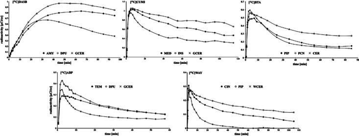
Images were analyzed using Matlab Release 2007b (The Mathworks, MA, USA) with extensions to FLIRT v5.2 (ref. 23), BET v1.2 (ref. 24), and SPM5 (Wellcome Department of Imaging Neuroscience, London, UK). Motion correction was applied. A RR and several anatomic target regions were traced based on brain atlases and published reports:^{25, 26} 6 ROI_DASB (midbrain; anterior cingulate; amygdala, AMY; dorsal putamen; hippocampus, HIP; thalamus; RR: gray-matter CER, GCER); 13 ROI_CUMI (HIP; entorhinal cortex; insula; posterior parahippocampal gyrus, PPH; temporal; AMY; medial prefrontal cortex, MED; cingulate, CIN; orbital; dorsolateral prefrontal cortex, DOR; parietal, PAR; raphe; occipital; RR: GCER); 6 ROI_BTA (CIN; parahippocampal gyrus, PIP; prefrontal cortex, PFC; HIP; PAR; precuneus; RR: CER); 14 ROI_ABP (CIN; DOR; temporal; AMY; dorsal caudate; dorsal putamen; HIP; ventral striatum, VST; inferior anterior cingulate, IAC; superior anterior cingulate; INS; orbital; MED; PAR; RR: GCER); and 13 ROI_WAY (raphe; anterior cingulate; AMY; CIN; DOR; HIP; INS; MED; occipital; orbital; PAR; PIP; temporal; RR: white CER, WCER). Selecting these ROIs restricted the analysis to regions for which the binding is expected to be relatively high. Figure 1 displays representative time activity curves (TACs) for the five radioligands.

Figure 1.

Representative time activity curves (TACs) and the reference region (RR) for the five considered radioligands: [¹¹C]DASB ([¹¹C]DASB), [¹¹C]CUMI-101 ([¹¹C]CUMI), [¹¹C]6-OH-BTA-1, Pittsburgh Compound-B ([¹¹C]BTA), [¹¹C]ABP688 ([¹¹C]ABP), and [¹¹C]WAY-100635 ([¹¹C]WAY). AMY, amygdala; CER, cerebellum; CIN, cingulate; DPU, dorsal putamen; GCER, gray-matter cerebellum; INS, insula; MED, medial prefrontal cortex; PCN, precuneus; PIP, parahippocampal gyrus; TEM, temporal; WCER, white CER.

Reference Region Approaches

Full reference tissue model. Although the first proposed RRA, FRTM^{1, 2, 3} has not been widely used in PET investigations due to poor convergence and computational time issues related to its relatively large number of free parameters and the noise present in the TACs. However, with increased computational power, a conservative constraint of some of these parameters (details below) allows now for an easy implementation of FRTM.

Assuming a one-tissue (1TC) and a two-tissue compartment (2TC) model for RR and target region, respectively, FRTM describes the total radioligand concentration time curve in the target region, C_T(t), and in the RR, C_R(t), through a set of linear differential equations, linking these concentration to cIF. The coefficients of these equations are (combination of) the transfer rate constants from plasma to free (K₁), free to plasma (k₂), free to specifically bound (k₃), and specifically bound to free compartment (k₄), respectively; and of the transfer rate constants from plasma to RR (), and vice versa ().

Assuming V_ND is constant throughout the brain (), a relationship is derived that links C_T(t) to C_R(t) without involving cIF:

where , a=(k₃+k₄−c)(c−r)/p, b=(dk₃−k₄)(d−r)/p, c=(s+p)/2, d=(s−p)/2, , q=4k₂k₄, r=k₂/R₁, s=k₁+k₂+k₃, and indicates the convolution operator. Using standard nonlinear regression techniques, R₁, k_2, k₃, and BP_ND=k₃/k₄ are estimated from C_T(t) and C_R(t).

In our implementation, estimates of R_1, c, and d, all positive by definition, are constrained accordingly.

Simplified reference tissue model. It was developed to improve FRTM slow convergence rates and the large variability of the estimates.^{3, 4} If the kinetics in the target region can be fitted satisfactorily with 1TC, then SRTM simplifies FRTM yielding:

R₁, k₂, and BP_ND are estimated from equation (2) using standard nonlinear regression.

Logan reference region. Logan graphical analysis²⁷ is based on the following transformation of C_T(t) and cIF (C_p(t)):

For t sufficiently large (t>t^*), V_T can be estimated as the slope β of the versus 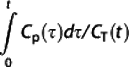plot. If equation (3) is applied to the RR, then 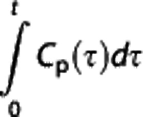can be expressed in terms of C_R(t) (or its integrals) and replaced in equation (3):

If the ratio C_R(t)/C_T(t) is reasonably constant over time, then Logan RR estimates BP_ND from the slope of the 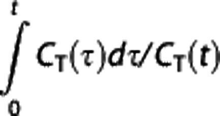versus 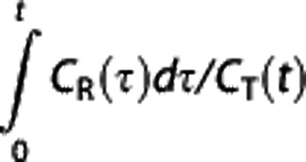plot as BP=(β/β′)−1 (ref. 5).

In this study, a common value for t^* (across ROIs or voxels, within the same radioligand) was chosen consistently with previous publications with the radioligands: this resulted in using the last eight frames for [¹¹C]DASB¹⁵ (t^*≈25 minutes after injection), [¹¹C]CUMI¹⁶ (t^*≈40 minutes), [¹¹C]ABP²¹ (t^*≈20 minutes), and [¹¹C]WAY²⁵ (t^*≈30 minutes); and the last six frames for [¹¹C]BTA^{17, 18} (t^*≈15 minutes).

Multilinear reference tissue model. Multilinear reference tissue model original MRTMo⁶ exploits the fact that equation (3) can be applied to both target region and RR for times in which the radioligand transport from plasma to tissue is unidirectional, thus yielding equation (4). Provided that , the partial regression coefficients β/β′, , and γ in equation (4) can be obtained by multiple regression analysis and BP_ND calculated as BP_ND=(β/β′)−1.

Multilinear reference tissue model. MRTM⁷ was proposed to overcome the bias of MRTMo estimates.^{7, 28} Ordinary least squares parameter estimation assumes that the independent variables are noise free. However, equation (4) contains a noisy term, C_T(t) in the independent variables, and the noise in the dependent and independent variables is correlated. Knowing that , equation (4) was arranged to yield:

where C_T(t) in the independent variables is replaced by its integral, which typically has much lower percent variation,²⁹ and the noise correlation in the dependent and independent variables is reduced. Nondisplaceable binding potential is calculated from the two regression coefficients θ₁=−β/(β′γ) and θ₂=1/γ as BP_ND=−((θ₁/θ₂)+1).

Multilinear reference tissue model 2. By using equation (5), for each target region a different is estimated as θ₁/θ₃, where , although theoretically there is only one true value. MRTM2 (ref 7) fixes to a value obtained from preliminary analysis to reduce the number of free parameters:

enables to estimate θ₁ and θ₂, and calculate BP_ND as with MRTM.

Likelihood estimation in graphical analysis with reference region. LEGA¹³ is an alternative approach to estimate the parameters in equation (3). It incorporates specific assumptions made on the measurement noise and gives optimal estimators of the slope β based on likelihood theory, thus yielding approximately unbiased V_T estimators.²⁵ It has been validated with [¹¹C]DASB test-retest data, proving to be the method of choice,¹⁵ and started to be considered as a viable alternative to traditional graphical analysis.³⁰ It is based on a rearrangement of equation (3):

for i=k, k+1, …, n, with k corresponding to t^*, the idealized ‘noise-free' data in the target region, t_i=(s_i−1+s_i)/2, with s_i the end point of the i^th PET scan frame, and the integrals expressed in terms of the values. If the errors with which all the actual Z_i observed (i.e., , i=1, 2, …, n) are assumed to be independent Gaussians, then the maximum likelihood estimator is obtained by minimizing via nonlinear optimization the quantity 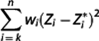over all β and γ, where the optimal weights w_i should be inversely proportional to the variances of the Z_i (e.g., .

Accordingly, equation (4) can be rewritten as:

with in the RR, and λ₁=β/β′, , λ₃=γ, and b_j functions of the time frame and previous and values: and , respectively. By solving equation (8) for and , a system of equations is obtained:

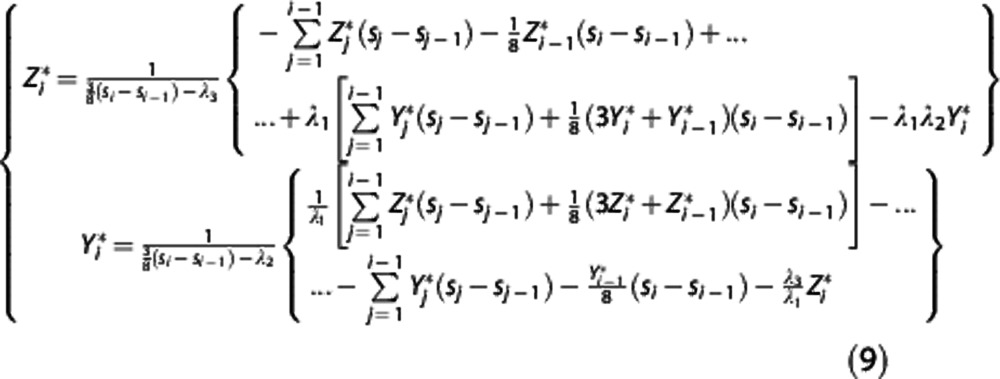In the implemented algorithm, is first expressed as a function of and for j<i (second equation in equation (9)); then the maximum likelihood estimator of is determined by minimizing, using 10% of the target regions, the quantity , where w_z,i and w_Y,i are optimal weights for target region and RR, respectively. With fixed, in each target region is then obtained by minimizing 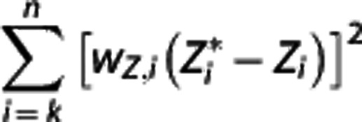over all λ₁, λ₂, and λ₃. Nondisplaceable binding potential is calculated as BP_ND=λ₁−1.

Bootstrap errors. At the ROI level, a bootstrap technique³¹ applied to the TACs data was used to determine the precision, expressed as standard error (SE), of the BP_ND estimates obtained by the RRAs. To generate the residuals to resample, the TAC in the RR was fitted with the model , with b₂=0.01. Fixing b₂ reduced the number of free parameters and assured convergence of the optimization routine across radioligands and subjects. The value for b₂ was empirically chosen based on preliminary analysis on a subset of subjects.

Outcome Measures and Performance Indices

Region of interest. In each subject and target region, BP_ND was estimated as BP_ND,IF=(V_T−V_T,RR)/V_T,RR, using the best available cIF-based method: LEGA for [¹¹C]DASB¹⁵ and [¹¹C]CUMI;¹⁶ Logan for [¹¹C]BTA;³² 2TC for [¹¹C]ABP;²¹ and constrained 2TC for [¹¹C]WAY.²² Nondisplaceable binding potential (BP_ND,REF) was also estimated using FRTM, SRTM, Logan RR, LEGA RR, MRTMo, MRTM, and MRTM2, with fixed in each subject as the average, MRTM2 (average), and the median, MRTM2 (median), values calculated across target regions within the subject with MRTMo.

The BP_ND,IF and BP_ND,REF were compared for each radioligand across target regions and subjects using: (1) correlation coefficient, r; (2) slope and intercept of the weighted regression line (BP_ND,IF the independent, BP_ND,REF the dependent variable); the reciprocals of the squares of the SE obtained by bootstrapping were used as weights; (3) mean and median percentage difference (PD): ; (4) mean and median coefficient of variation (CV) (calculated from the SE).

Voxel. For each radioligand, 10 subjects were randomly selected, as an exhaustive analysis on the whole data set was prohibitive in terms of computational demand. The BP_ND,REF images were generated with SRTM, Logan RR, LEGA RR, MRTMo, MRTM, and MRTM2 (average). We considered the SRTM implementation by Gunn et al,³³ which, by using a set of basis functions and enabling parameter bounding based on a priori knowledge of each radioligand, is more stable and faster than nonlinear least squares estimation. Full reference tissue model and MRTM2 (median) were not considered because of convergence issues (FRTM cannot be efficiently applied at the voxel level), and redundancy with the MRTM2 (average) results, respectively.

Results were compared for each radioligand across subjects using: (1) r between BP_ND,IF (from ROI) and the average of the BP_ND values estimated within each target region from the images (BP_ND,im); (2) slope and intercept of the weighted regression line (BP_ND,IF the independent, BP_ND,im the dependent variable); the squared reciprocals of the standard deviation (SD) of the BP_ND values estimated within each target region from the images were used as weights; (3) CV of the BP_ND values (calculated from the SD).

Outlier detection. At both ROI and voxel level, first a weighted regression line was fitted by considering BP_ND,IF and BP_ND,REF (or BP_ND,im) in all target regions and subjects for each radioligand. Weighted studentized residuals were then calculated as , where is the i^th residual, an appropriate estimate of the residuals SD, and h_ii the i^th diagonal entry in the hat matrix. Any estimate with absolute studentized residual over 3 was excluded from the following weighted regression analysis, whose results are reported here together with the percentage of outliers excluded.

Criteria and presentation of the results. We report several indices that can help other investigators selecting the most suitable RRA for their studies. When compared with cIF results, we would expect a good RRA to have high correlation (i.e., RRA results match the corresponding cIF ones as closely as possible) and accuracy (i.e., low bias in the estimates). In addition, a good RRA should have high precision (i.e., low CV) and it should also not result in many outliers. Often a single RRA does not meet all these requirements, so compromise is necessary in practice. For example, with a small data set, RRAs with a low percentage of outliers might be preferable, while accuracy and correlation are more important when replicating or consolidating results previously obtained with cIF quantification; precision is important for PET studies involving multiple scans on the same subject (e.g., occupancy studies).

The following sections focus mostly on the results obtained by RRAs meeting specific minimum performance levels: correlation r higher than 0.5; slope between 0.7 and 1.3 (i.e., maximum relative bias of 30%); median PD lower than 50% and percentage of outliers lower than 2%. These thresholds were independently selected a priori across radioligands and RRAs, based on our experience with PET data analysis. However, as the assessment of a given RRA performance also depends on factors such as study design and overall goal, we made available (Supplementary Material) all the results for each radioligand and RRA.

Results

Region of Interest Analysis

Table 1 (ROI section) reports the numerical results for those RRAs that meet the criteria laid out in Materials and methods. Any RRA not meeting the minimal requirements is said to fail for that particular radioligand. Complete results are reported in Supplementary Table A.

Table 1. ROI analysis and voxel analysis.

	ROI					Voxel
	r	Slope	Outliers %	Median PD	Median CV	r	Slope	Outliers %	Median CV
[11C]DASB (N=209)
FRTM	0.958	0.969	0.80	7.488	0.191		—		—
SRTM	0.972	0.933	0.16	6.596	0.136		—		—
Logan RR	0.956	0.703	1.59	22.603	0.111		—		—
MRTM	0.973	0.947	1.83	7.182	0.143	0.508	0.833	0.91	5.401
[11C]CUMI (N=22)
FRTM	0.982	0.986	1.05	4.914	0.045		—		—
SRTM	0.994	0.958	1.05	6.103	0.039		—		—
MRTM	0.702	0.989	0.70	5.215	0.059		—		—
MRTMo	—	—	—	—	—	0.902	0.703	1.20	0.692
LEGA RR	—	—	—	—	—	0.947	0.901	1.60	0.733
[11C]BTA (N=74)
SRTM	0.705	0.886	0.23	24.288	0.056		—		—
MRTM	0.649	0.868	0.23	20.967	0.120		—		—
MRTM2 (average)	0.984	0.872	0.68	19.556	0.088		—		—
MRTM2 (median)	0.983	0.878	0.68	19.582	0.088		—		—
LEGA RR	—	—	—	—	—	0.990	0.863	0.00	1.044
[11C]ABP (N=41)
MRTM2 (average)	0.856	0.747	1.92	8.156	0.088		—		—
MRTM2 (median)	0.852	0.726	1.74	8.037	0.085		—		—
LEGA RR	—	—	—	—	—	0.909	0.885	0.00	0.772
[11C]WAY (N=287)
MRTM2 (median)	0.608	0.831	0.32	26.374	0.036		—		—

CV, coefficient of variation; FRTM, full reference tissue model; LEGA, likelihood estimation in graphical analysis; MRTM, multilinear reference tissue model; PD, percentage difference; ROI, region of interest; RR, reference region; SRTM, simplified reference tissue model.

ROI analysis: correlation, weighted regression analysis, percentage of outliers, PD, and CV results organized by radioligand. Voxel analysis: correlation, weighted regression analysis, percentage of outliers, and CV results organized by radioligand. Only the RRAs and radioligands matching the requirements laid out in Materials and methods are included.

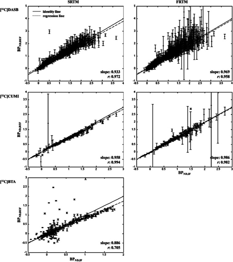
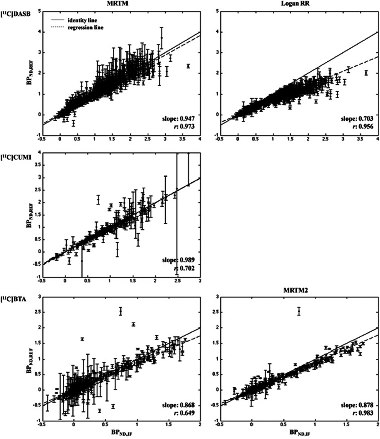
[¹¹C]DASB. Figure 2 (top) shows the scatter plots of BP_ND,IF and BP_ND,REF for FRTM and SRTM. Full reference tissue model shows the highest slope among the RRAs (0.969; refer to Table 1), the second lowest percentage of outliers (0.80%), PD values comparable to those with SRTM, which shows the lowest PD values among RRAs for [¹¹C]DASB (∼7.4% versus ∼6.6%), but the highest median CV (∼0.19). Simplified reference tissue model improves the performance of FRTM (higher correlation, lower percentage of outliers and median CV) at the price of a more pronounced BP_ND underestimation. Figure 3 (top) shows the same scatter plots for Logan RR and MRTM. As shown by the values reported in Table 1, MRTM performs similarly to FRTM and SRTM in terms of correlation (0.973), accuracy (slope: 0.947; median PD: ∼7.2%), and precision (median CV: ∼0.14), at the price of the highest percentage of outliers for this radioligand (1.83%). Logan RR shows the worst slope and median PD, although the lowest median CV. Correlation values are high across the RRAs.

Figure 2.

Region of interest (ROI) analysis: simplified reference tissue model (SRTM) and full reference tissue model (FRTM). Scatter plots of BP_ND,IF (X-axis) and BP_ND,REF (Y-axis) for [¹¹C]DASB (top; 209 × ROI_DASB=1,254 cases), [¹¹C]CUMI (middle; 22 × ROI_CUMI=286 cases), and [¹¹C]BTA (bottom; 74 × ROI_BTA=444 cases). The X-axis is the full cIF analysis (LEGA for [¹¹C]DASB and [¹¹C]CUMI; Logan for [¹¹C]BTA). In each plot, the identity (solid) and the weighted regression (dashed) lines are reported. Each point bars represent the standard error (SE) of the corresponding BP_ND estimate. BP_ND, nondisplaceable binding potential; IF, input function; cIF, metabolite-corrected IF; LEGA, likelihood estimation in graphical analysis.

Figure 3.

Region of interest (ROI) analysis: MRTM, Logan RR, and MRTM2. Scatter plots of BP_ND,IF (X-axis) and BP_ND,REF (Y-axis) for [¹¹C]DASB (top; 209 × ROI_DASB=1,254 cases), [¹¹C]CUMI (middle; 22 × ROI_CUMI=286 cases), and [¹¹C]BTA (bottom; 74 × ROI_BTA=444 cases). The X-axis is the full cIF analysis (LEGA for [¹¹C]DASB and [¹¹C]CUMI; Logan for [¹¹C]BTA). In each plot, the identity (solid) and the weighted regression (dashed) lines are reported. Each point bars represent the standard error (SE) of the corresponding BP_ND estimate. BP_ND, nondisplaceable binding potential; MRTM, multilinear reference tissue model; RR, reference region; IF, input function; cIF, metabolite-corrected IF; LEGA, likelihood estimation in graphical analysis.

[¹¹C]CUMI. Figure 2 (middle) shows the scatter plots for FRTM and SRTM; Figure 3 (middle) reports the scatter plot for MRTM. Multilinear reference tissue model and FRTM provide similar slope values (0.989 and 0.986, respectively; Table 1), but different correlation (0.702 and 0.982). Simplified reference tissue model performs similarly to FRTM, with a slightly higher underestimation of BP_ND (slope: 0.958).

[¹¹C]BTA. Figure 2 (bottom) shows the scatter plots for SRTM, while Figure 3 (bottom) reports the scatter plot for MRTM and MRTM2 methods (MRTM2 median is shown as representative). As reported in Table 1, MRTM2 methods show the highest correlation and PD; in terms of slope and CV, they perform better than MRTM but worse than SRTM, at the price of higher percentage of outliers.

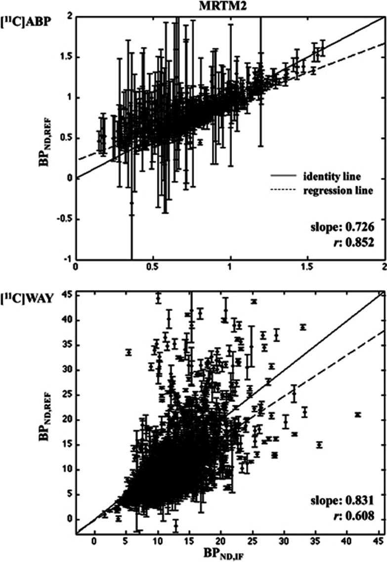
[¹¹C]ABP and [¹¹C]WAY. The MRTM2 methods are the only RRAs meeting the requirements with [¹¹C]ABP, and their performance is very close (Table 1). Figure 4 (top) reports the scatter plot only for MRTM2 (median) as representative of both approaches. Only MRTM2 (median) meets the criteria for [¹¹C]WAY (Figure 4, bottom).

Figure 4.

Region of interest (ROI) analysis: MRTM2. Scatter plots of BP_ND,IF (X-axis) and BP_ND,REF (Y-axis) for [¹¹C]ABP (top; 41 × ROI_ABP=574 cases) and [¹¹C]WAY (bottom; 287 × ROI_WAY=3,731 cases). The X-axis is the full cIF analysis (2TC for [¹¹C]ABP; 2TCC for [¹¹C]WAY). In each plot, the identity (solid) and the weighted regression (dashed) lines are reported. Each point bars represent the standard error (SE) of the corresponding BP_ND estimate. BP_ND, nondisplaceable binding potential; cIF, metabolite-corrected IF; IF, input function; MRTM, multilinear reference tissue model; 2TC, two-tissue compartment; 2TCC, constrained 2TC.

Voxel Analysis

Table 1 (voxel section) reports the numerical results for the RRAs meeting the criteria laid out in Materials and methods. Complete results are reported in Supplementary Table B.

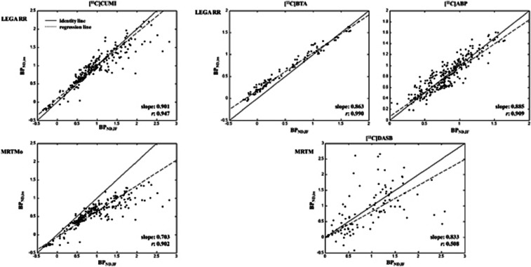
[¹¹C]DASB. Figure 5 (right panel) shows the scatter plots of BP_ND,IF and BP_ND,im with MRTM, which performs poorly in terms of correlation and precision, as reported in Table 1.

Figure 5.

Voxel analysis: LEGA RR, MRTMo, and MRTM. Scatter plots of BP_ND,IF (X-axis; region of interest (ROI) analysis) and BP_ND,im (Y-axis; average within each target region) for 10 randomly selected subjects for [¹¹C]CUMI (left panel), [¹¹C]BTA, [¹¹C]ABP, and [¹¹C]DASB (right panel). The X-axis is the full cIF (ROI) analysis (LEGA for [¹¹C]DASB and [¹¹C]CUMI; Logan for [¹¹C]BTA); 2TC for [¹¹C]ABP). BP_ND, nondisplaceable binding potential; cIF, metabolite-corrected IF; IF, input function; LEGA, likelihood estimation in graphical analysis; MRTM, multilinear reference tissue model; RR, reference region; 2TC, two-tissue compartment.

[¹¹C]CUMI. Figure 5 (left panel) shows the scatter plots with LEGA RR and MRTMo. According to Figure 5 and the values in Table 1, LEGA RR performs the best in terms of correlation (0.947) and slope (0.901), at the price of slightly higher percentage of outliers (1.60% versus 1.20%) and increased variability (median CV: ∼0.73 versus ∼0.69) compared with MRTMo.

[¹¹C]BTA and [¹¹C]ABP. Figure 5 (right panel) shows the scatter plots with LEGA RR for these two radioligands.

[¹¹C]WAY. None of the RRAs considered performs well for this radioligand at the voxel level.

Discussion

Region of Interest Analysis

We consider the RRAs performance from two perspectives: for each radioligand, we summarize which methods tend to provide good estimates; and for each method, we summarize its performance on the various radioligands.

Radioligands perspective. According to our criteria and the results obtained, the radioligands considered here tend to cluster into two groups based on the average performance achieved by the various RRAs with these radioligands, and their RR kinetic behavior.

[¹¹C]DASB, [¹¹C]CUMI, and [¹¹C]BTA. Overall, results suggest that RRAs can be satisfactorily applied to analyze ROI data of [¹¹C]DASB, [¹¹C]CUMI, and [¹¹C]BTA. Kinetic modeling with FRTM and SRTM shows good accuracy and correlation (although performance worsens with [¹¹C]BTA), and acceptable precision. Alternatively, MRTM and MRTM2 perform similarly to FRTM and SRTM, although again with poorer performance for [¹¹C]BTA.

[¹¹C]ABP and [¹¹C]WAY. Radioligands like [¹¹C]ABP and [¹¹C]WAY may represent a challenge for RRAs: results suggest that RRAs should not be applied, as very poor performance is seen at the ROI level. MRTM2 methods, the only RRAs meeting the requirements for these radioligands, provide high correlation, but relatively poor accuracy, with [¹¹C]ABP, and vice versa (good accuracy, but low correlation) with [¹¹C]WAY. With these radioligands, an alternative to cIF analysis may still be represented by minimally invasive fully quantitative approaches like simultaneous estimation of the cIF,³⁴ which requires just one arterial blood sample.

Trends in the reference region approaches. The same ‘groups' can be seen when sorting the considered radioligands according to the average values of and V_T,RR (as estimated by 1TC with cIF) across all subjects within the same radioligand. The average V_T,RR is relatively high for [¹¹C]DASB (9.49±1.94; SD values across all subjects within the same radioligand), [¹¹C]CUMI (6.29±2.51) and, to a certain degree, [¹¹C]BTA (1.54±0.30), while it decreases below 1 for [¹¹C]ABP (0.93±0.26) and [¹¹C]WAY (0.29±0.10). Corresponding average shows the same trend (0.51±0.11 [¹¹C]DASB; 0.25±0.06 [¹¹C]CUMI; 0.12±0.02 [¹¹C]BTA; 0.06±0.02 [¹¹C]ABP; 0.04±0.02 [¹¹C]WAY). [¹¹C]DASB and [¹¹C]CUMI, and [¹¹C]BTA and [¹¹C]ABP, respectively, switch positions when sorted according to increasing average values of (1TC with cIF): average is relatively low for [¹¹C]CUMI (0.04±0.01) and [¹¹C]DASB (0.05±0.01), increases for [¹¹C]ABP (0.07±0.01) and [¹¹C]BTA (0.08±0.02), and doubles for [¹¹C]WAY (0.15±0.06).

We investigated how, on average, RRAs correlation, accuracy, and precision (as assessed in the ROI analysis) vary according to the average V_T,RR, , and (as calculated with cIF and 1TC) of these radioligands. On average across RRAs, the correlation obtained for a specific radioligand increases for higher values of V_T,RR and , and lower values of . Please refer to Supplementary Figure A for a plot of average (±SD) of the correlation (r) values (across all RRAs and within each radioligand; all ROI results from Supplementary Table A are included) versus the average (±SD) values of V_T,RR, , and of each radioligand. Also accuracy increases for higher values of V_T,RR and , and lower values of (Supplementary Figure B). It is not unexpected that no trend seems to be present for the precision, which is more likely to be affected by the noise in the TACs.

According to the reported criteria and the results obtained, we therefore suggest that, although certainly many factors contribute to the performance of each RRA, the kinetics in the RR may have a role, and that RRAs on average seem to prefer radioligands with higher V_T,RR and , and lower .

Reference region approaches perspective. The ROI analysis results can be analyzed from the point of view of how each RRA performs across the considered radioligands.

Full reference tissue model. Full reference tissue model performs well with [¹¹C]DASB and [¹¹C]CUMI. The best performance (correlation: ∼0.98; accuracy: slope ∼0.99; median PD ∼5%) corresponds to [¹¹C]CUMI, although with a slightly higher percentage of outliers (1.05%) as compared with [¹¹C]DASB. We attribute the high percentage of outliers produced by FRTM more to noise in the TACs, which affects the convergence in the optimization process in the estimation of FRTM parameters, than to violations in the modeling assumptions. Similarly, precision, which is an issue with FRTM for many of the considered radioligands, is more likely related to convergence issues in the optimization procedure.

Simplified reference tissue model. It performs well with [¹¹C]DASB, [¹¹C]CUMI, and to a certain degree (correlation and accuracy worsen) [¹¹C]BTA. Given one of its assumptions—that the target region TACs can be fitted satisfactorily with 1TC with cIF—it is not surprising that SRTM works well for [¹¹C]DASB, whose kinetics can be described by 1TC.¹⁵ Simplified reference tissue model in fact achieves significantly better correlation, accuracy, and lower percentage of outliers for [¹¹C]DASB, as compared with [¹¹C]ABP (whose cIF-based best method is 2TC), [¹¹C]BTA (Logan), and [¹¹C]WAY (constrained 2TC). The CV values follow a different trend, as SRTM shows the highest median CV with [¹¹C]DASB. However, in the case of precision, performances are likely to be more affected by noise in each TAC rather than violations in the modeling assumptions. Although [¹¹C]CUMI kinetics are generally described better by 2TC than by 1TC,¹⁶ the main difference in the two models' fits lies in the initial peak portion of the TACs, while the tail is well fit by both. As a result, average and SD values (across subjects) of V_T (and BP_ND) estimated in each region by the two models are close to each other and to the estimates obtained by LEGA, which is the method of choice for [¹¹C]CUMI.¹⁶

Considering [¹¹C]DASB and [¹¹C]CUMI, SRTM provides better correlation than FRTM ([¹¹C]DASB: 0.972 versus 0.958; [¹¹C]CUMI 0.994 versus 0.982). Inversely, FRTM provides better accuracy than SRTM (the slope is the closest to unity for [¹¹C]DASB, ∼0.97 and among the closest for [¹¹C]CUMI, ∼0.99) at the price of slightly lower precision (i.e., higher CV). Simplified reference tissue model shows better slope (∼0.89) and precision (median CV ∼0.06) but worse PD (∼24%) than the graphical approaches (MRTM2 methods) with [¹¹C]BTA.

Logan reference region. Logan RR meets the criteria only with [¹¹C]DASB, for which it shows good correlation at the expense of accuracy (slope: ∼0.7; median PD: ∼23%). Logan RR ‘fails' for poor accuracy and high percentage of outliers. Logan RR underestimates BP_ND the most for all the considered radioligands, except [¹¹C]ABP (Supplementary Table A). Overall, investigators should balance the good correlation of Logan RR with its significant BP_ND underestimation.

MRTMo. MRTMo does not meet the criteria for any of the five radioligands at the ROI level. MRTMo behaves similarly to the other two graphical approaches, Logan RR and LEGA RR. More precisely, MRTMo overall shows better correlation and accuracy than Logan RR and, in some cases, LEGA RR, but at the price of significantly increased percentage of outliers and worse estimates precision. MRTMo ‘fails' mostly for percentage of outliers.

Multilinear reference tissue model. It meets the requirements with [¹¹C]DASB, [¹¹C]CUMI, and [¹¹C]BTA, although with [¹¹C]BTA correlation and accuracy worsen. As any method trying to overcome the BP_ND underestimation of Logan RR,^{7, 28} MRTM reduces the BP_ND underestimation, at the expense of considerably decreased correlation and increased variability.

Multilinear reference tissue model 2. Both versions of MRTM2 work well with [¹¹C]ABP and [¹¹C]BTA. Only MRTM2 (median) also satisfies the requirements for [¹¹C]WAY, but with poor correlation (∼0.61) and high PD values (∼26%). As expected from results by Ichise et al,⁷ MRTM2 approaches maintain accuracy similar to MRTM (or at least better than MRTMo), while improving correlation and precision of the estimates. The MRTM2 accuracy lowers with [¹¹C]ABP and [¹¹C]WAY, although precision remains high, especially with [¹¹C]WAY. The choice of certainly has a role in MRTM2 performance and further investigation may provide a more sophisticated approach to accurately select to improve MRTM2 results for these and other radioligands.

Likelihood estimation in graphical analysis with reference region. Likelihood estimation in graphical analysis RR is excluded from consideration at the ROI level because it shows too many outliers, although it crosses the selected threshold only by a small margin with those radioligands for which RRAs are suggested (2.07%, [¹¹C]DASB; 2.45% [¹¹C]CUMI; 2.48%, [¹¹C]BTA) (Supplementary Table A). Neglecting the outlier issue, with both [¹¹C]DASB and [¹¹C]CUMI LEGA RR performs similarly to FRTM for correlation (∼ 0.96 and∼0.99) and to SRTM for median PD (∼7.5% and ∼6%), but shows a lower slope value (∼0.83 and 0.94). With [¹¹C]BTA, LEGA RR shows correlation even higher than the MRTM2 methods (∼0.99), but a lower slope (∼0.79) and higher median PD (∼22%). With those radioligands for which RRAs are not suggested, LEGA RR does not meet the criteria only for the slope (0.527), with [¹¹C]ABP, and both slope (0.412) and median PD (∼55%) with [¹¹C]WAY. Despite this, LEGA RR shows correlation (∼0.90, [¹¹C]ABP; ∼0.83, [¹¹C]WAY) comparable or higher than the MRTM2 approaches.

Voxel Analysis

Full reference tissue model cannot be efficiently applied at the voxel level because of the noise in the TACs, which affects the convergence in the optimization process required in the estimation of the parameters, and computational time. An alternative linear implementation has not yet been proposed.

Simplified reference tissue model does not seem appropriate for application at the voxel level because it tends to fail for poor accuracy for all five radioligands (slope ∼0.66—[¹¹C]DASB; ∼0.58—[¹¹C]CUMI; ∼0.59—[¹¹C]BTA; ∼0.64—[¹¹C]ABP; ∼0.23—[¹¹C]WAY). However, further optimization for a specific radioligand of the algorithm proposed (and here applied) by Gunn et al³³ would probably improve SRTM's accuracy and potentially make the analysis of voxel data possible.

Also Logan RR does not seem appropriate for the voxel analysis for all five radioligands, but only for poor accuracy (Supplementary Table B).

The MRTM, another candidate at the ROI level for the analysis of [¹¹C]DASB, [¹¹C]CUMI, and [¹¹C]BTA, shows poor performance at the voxel level with [¹¹C]DASB (correlation: ∼0.5; slope: ∼0.8), and ‘fails' the analysis with [¹¹C]CUMI (correlation ∼0.11, slope ∼0.61) and [¹¹C]BTA (slope ∼0.61, outliers 2.5%). The MRTM performance is generally poor for all five radioligands (correlation range: 0.1 to 0.63; slope range: 0.29 to 0.84).

Likelihood estimation in graphical analysis with RR is the only RRA in this study that performs well for more than one radioligand at the voxel level ([¹¹C]CUMI, [¹¹C]BTA, and [¹¹C]ABP), showing good correlation, accuracy, and precision, with no or very few excluded outliers (Table 1). The method performance at the ROI and voxel level is reasonably close. With [¹¹C]DASB, LEGA RR does not meet the criteria only for the percentage of outliers (3.64%), while correlation and slope slightly improve with respect to the ROI analysis (Supplementary Table B). Also with [¹¹C]CUMI performance is close: correlation decreases (0.987 versus 0.947), slope decreases (0.945 versus 0.901), and the percentage of outliers slightly decreases (from 2.45% to 1.60%, enough to satisfy the criteria). With [¹¹C]BTA, correlation stays high (0.993 versus 0.990), slope improves (0.794 versus 0.863), and the percentage of outliers decreases to 0%. With [¹¹C]ABP, correlation is very close (0.898 versus 0.909), slope improves (0.527—below versus 0.885—above the threshold), while the percentage of outliers decreases from 0.7% to 0%. With [¹¹C]WAY, correlation is close (0.830 versus 0.847), slope decreases (0.412 versus 0.395—both below the threshold), and the percentage of outliers slightly increases (0.78% versus 1.2%).

Other RRAs show higher percentages of outliers at the ROI versus the voxel level. MRTMo, for example, shows a higher percentage of outliers in the ROI analysis with all the considered radioligands. Logan RR shows higher percentage at the ROI level with all the radioligands, except [¹¹C]DASB. Simplified reference tissue model, MRTM, and MRTM2 (average) present higher percentages of outliers at the ROI level in few cases, although not consistently across radioligands. Keeping in mind that an outlier at the ROI level is potentially quite different from one at the voxel level, one possible explanation is that the voxel BP_ND estimates are noisier (i.e., the Y-axis in the BP_ND scatter plots); therefore, the estimated regression SD is large enough to where fewer points (proportionally speaking) are identified as outliers.

MRTMo matches the requirements only with [¹¹C]CUMI at the voxel level, in which case it performs worse than LEGA RR. The MRTM2 ‘fails' with all the considered radioligands. No RRA performs well for [¹¹C]WAY.

The RRAs not meeting the requirements were excluded most often for poor accuracy, but sometimes for low correlation and high percentage of outliers. As estimation at the voxel level presents per se challenges that are related to the noisier nature of the signal rather than the adopted estimation approach, RRAs will certainly benefit from any methodological improvement able to solve the increased underestimation and variability of the estimates of any approach applied at the voxel level.

Conclusions

Given the range of correlation, accuracy, and precision achieved, and according to our criteria, results suggest that RRAs can be used to analyze [¹¹C]DASB, [¹¹C]CUMI, and [¹¹C]BTA (and potentially similar radioligands), but not the other considered radioligands. However, the assessment of any RRA performance also depends on the specific aims of each study; therefore, several indices are reported that can help other investigators selecting the most suitable approach.

Although the newly presented LEGA RR is excluded from consideration for ROI analysis because it shows too many outliers, its good performance at the voxel level suggests that it can generate smooth parametric images that are highly correlated with BP_ND,IF, minimally biased, and can be facilely used in statistical or group analysis (e.g., SPM), without the need for a priori knowledge of each radioligand behavior as with SRTM.³³

The use of bootstrap errors,¹⁴ for the first time here introduced for RRAs, can help in the selection between competing methods by adding a measure of precision to the BP_ND estimates. It also allows investigators to weight each BP_ND estimate according to its reliability in subsequent group analysis.

The authors declare no conflict of interest.

References

- Cunningham VJ, Hume SP, Price GR, Ahier RG, Cremer JE, Jones AK. Compartmental analysis of diprenorphine binding to opiate receptors in the rat in vivo and its comparison with equilibrium data in vitro. J Cereb Blood Flow Metab. 1991;11:1–9. doi: 10.1038/jcbfm.1991.1. [DOI] [PubMed] [Google Scholar]
- Hume SP, Myers R, Bloomfield PM, Opacka-Juffry J, Cremer JE, Ahier RG, et al. Quantitation of carbon-11-labeled raclopride in rat striatum using positron emission tomography. Synapse. 1992;12:47–54. doi: 10.1002/syn.890120106. [DOI] [PubMed] [Google Scholar]
- Lammertsma AA, Bench CJ, Hume SP, Osman S, Gunn K, Brooks DJ, et al. Comparison of methods for analysis of clinical [11C]raclopride studies. J Cereb Blood Flow Metab. 1996;16:42–52. doi: 10.1097/00004647-199601000-00005. [DOI] [PubMed] [Google Scholar]
- Lammertsma AA, Hume SP. Simplified reference tissue model for PET receptor studies. Neuroimage. 1996;4:153–158. doi: 10.1006/nimg.1996.0066. [DOI] [PubMed] [Google Scholar]
- Logan J, Fowler JS, Volkow ND, Wang GJ, Ding YS, Alexoff DL. Distribution volume ratios without blood sampling from graphical analysis of PET data. J Cereb Blood Flow Metab. 1996;16:834–840. doi: 10.1097/00004647-199609000-00008. [DOI] [PubMed] [Google Scholar]
- Ichise M, Ballinger JR, Golan H, Vines D, Luong A, Tsai S, et al. Noninvasive quantification of dopamine D2 receptors with Iodine-123-IBF SPECT. J Nucl Med. 1996;37:513–520. [PubMed] [Google Scholar]
- Ichise M, Liow JS, Lu JQ, Takano A, Model K, Toyama H, et al. Linearized reference tissue parametric imaging methods: application to [11C]DASB positron emission tomography studies of the serotonin transporter in human brain. J Cereb Blood Flow Metab. 2003;23:1096–1112. doi: 10.1097/01.WCB.0000085441.37552.CA. [DOI] [PubMed] [Google Scholar]
- Innis RB, Cunningham VJ, Delforge J, Fujita M, Gjedde A, Gunn RN, et al. Consensus nomenclature for in vivo imaging of reversibly binding radioligands. J Cereb Blood Flow Metab. 2007;27:1533–1539. doi: 10.1038/sj.jcbfm.9600493. [DOI] [PubMed] [Google Scholar]
- Slifstein M, Laruelle M. Models and methods for derivation of in vivo neuroreceptor parameters with PET and SPECT reversible radiotracers. Nucl Med Biol. 2001;28:595–608. doi: 10.1016/s0969-8051(01)00214-1. [DOI] [PubMed] [Google Scholar]
- Parsey RV, Arango V, Olvet DM, Oquendo MA, Van Heertum RL, Mann JJ. Regional heterogeneity of 5-HT1A receptors in human cerebellum as assessed by positron emission tomography. J Cereb Blood Flow Metab. 2005;25:785–793. doi: 10.1038/sj.jcbfm.9600072. [DOI] [PubMed] [Google Scholar]
- Parsey RV, Ogden RT, Miller JM, Tin A, Hesselgrave N, Goldstein E, et al. Higher serotonin 1A binding in a second major depression cohort: modeling and reference region considerations. Biol Psychiatry. 2010;68:170–178. doi: 10.1016/j.biopsych.2010.03.023. [DOI] [PMC free article] [PubMed] [Google Scholar]
- Oquendo MA, Hastings RS, Huang YY, Simpson N, Ogden RT, Hu XZ, et al. Brain serotonin transporter binding in depressed patients with bipolar disorder using positron emission tomography. Arch Gen Psychiatry. 2007;64:201–208. doi: 10.1001/archpsyc.64.2.201. [DOI] [PMC free article] [PubMed] [Google Scholar]
- Ogden RT. Estimation of kinetic parameters in graphical analysis of PET imaging data. Stat Med. 2003;22:3557–3568. doi: 10.1002/sim.1562. [DOI] [PubMed] [Google Scholar]
- Ogden RT, Ojha A, Erlandsson K, van Heertum R, Mann JJ, Parsey RV. Using bootstrap identifiability as a metric for model selection for dynamic [11C]DASB PET data. IEEE Nucl Sci Symp Conf Rec. 2005;M11-276:2636–2639. [Google Scholar]
- Ogden RT, Ojha A, Erlandsson K, Oquendo MA, Mann JJ, Parsey RV. In vivo quantification of serotonin transporters using [(11)C]DASB and positron emission tomography in humans: modeling considerations. J Cereb Blood Flow Metab. 2007;27:205–217. doi: 10.1038/sj.jcbfm.9600329. [DOI] [PMC free article] [PubMed] [Google Scholar]
- Milak MS, DeLorenzo C, Zanderigo F, Prabhakaran J, Kumar JS, Majo VJ, et al. In vivo quantification of human serotonin 1A receptor using 11C-CUMI-101, an agonist PET radiotracer. J Nucl Med. 2010;51:1892–1900. doi: 10.2967/jnumed.110.076257. [DOI] [PMC free article] [PubMed] [Google Scholar]
- Mikhno A, Devanand D, Pelton G, Cuasay K, Gunn R, Upton N, et al. Voxel-based analysis of 11C-PIB scans for diagnosing Alzheimer's disease. J Nucl Med. 2008;49:1262–1269. doi: 10.2967/jnumed.107.049932. [DOI] [PMC free article] [PubMed] [Google Scholar]
- Devanand DP, Mikhno A, Pelton GH, Cuasay K, Pradhaban G, Dileep Kumar JS, et al. Pittsburgh compound B (11C-PIB) and fluorodeoxyglucose (18 F-FDG) PET in patients with Alzheimer disease, mild cognitive impairment, and healthy controls. J Geriatr Psychiatry Neurol. 2010;23:185–198. doi: 10.1177/0891988710363715. [DOI] [PMC free article] [PubMed] [Google Scholar]
- Bélanger MJ, Simpson NR, Wang T, Van Heertum RL, Mann JJ, Parsey RV. Biodistribution and radiation dosimetry of [11C]DASB in baboons. Nucl Med Biol. 2004;31:1097–1102. doi: 10.1016/j.nucmedbio.2004.09.002. [DOI] [PubMed] [Google Scholar]
- Milak MS, Severance AJ, Ogden RT, Prabhakaran J, Kumar JS, Majo VJ, et al. Modeling considerations for 11C-CUMI-101, an agonist radiotracer for imaging serotonin 1A receptor in vivo with PET. J Nucl Med. 2008;49:587–596. doi: 10.2967/jnumed.107.046540. [DOI] [PMC free article] [PubMed] [Google Scholar]
- Ametamey SM, Treyer V, Streffer J, Wyss MT, Schmidt M, Blagoev M, et al. Human PET studies of metabotropic glutamate receptor subtype 5 with 11C-ABP688. J Nucl Med. 2007;48:247–252. [PubMed] [Google Scholar]
- Parsey RV, Slifstein M, Hwang DR, Abi-Dargham A, Simpson N, Mawlawi O, et al. Validation and reproducibility of measurement of 5-HT1A receptor parameters with [carbonyl-11C]WAY-100635 in humans: comparison of arterial and reference tissue input functions. J Cereb Blood Flow Metab. 2000;20:1111–1133. doi: 10.1097/00004647-200007000-00011. [DOI] [PubMed] [Google Scholar]
- Jenkinson M, Smith S. A global optimisation method for robust affine registration of brain images. Med Image Anal. 2001;5:143–156. doi: 10.1016/s1361-8415(01)00036-6. [DOI] [PubMed] [Google Scholar]
- Smith SM. Fast robust automated brain extraction. Hum Brain Mapp. 2002;17:143–155. doi: 10.1002/hbm.10062. [DOI] [PMC free article] [PubMed] [Google Scholar]
- Parsey RV, Ogden RT, Mann JJ. Determination of volume of distribution using likelihood estimation in graphical analysis: elimination of estimation bias. J Cereb Blood Flow Metab. 2003;23:1471–1478. doi: 10.1097/01.WCB.0000099460.85708.E1. [DOI] [PubMed] [Google Scholar]
- Parsey RV, Ojha A, Ogden RT, Erlandsson K, Kumar D, Landgrebe M, et al. Metabolite considerations in the in vivo quantification of serotonin transporters using 11C-DASB and PET in humans. J Nucl Med. 2006;47:1796–1802. [PubMed] [Google Scholar]
- Logan J, Fowler JS, Volkow ND, Wolf AP, Dewey SL, Schlyer DJ, et al. Graphical analysis of reversible radioligand binding from time-activity measurements applied to [N-11C-methyl]-(-)-cocaine PET studies in human subjects. J Cereb Blood Flow Metab. 1990;10:740–747. doi: 10.1038/jcbfm.1990.127. [DOI] [PubMed] [Google Scholar]
- Slifstein M, Laruelle M. Effects of statistical noise on graphic analysis of PET neuroreceptor studiesJ. J Nucl Med. 2000;41:2083–2088. [PubMed] [Google Scholar]
- Ichise M, Toyama H, Innis RB, Carson RE. Strategies to improve neuroreceptor parameter estimation by linear regression analysis. J Cereb Blood Flow Metab. 2002;22:1271–1281. doi: 10.1097/01.WCB.0000038000.34930.4E. [DOI] [PubMed] [Google Scholar]
- Joshi A, Fessler JA, Koeppe RA. Improving PET receptor binding estimates from Logan plots using principal component analysis. J Cereb Blood Flow Metab. 2008;28:852–865. doi: 10.1038/sj.jcbfm.9600584. [DOI] [PMC free article] [PubMed] [Google Scholar]
- Ogden RT, Tarpey T. Estimation in regression models with externally estimated parameters. Biostatistics. 2006;7:115–129. doi: 10.1093/biostatistics/kxi044. [DOI] [PubMed] [Google Scholar]
- Price JC, Klunk WE, Lopresti BJ, Lu X, Hoge JA, Ziolko SK, et al. Kinetic modeling of amyloid binding in humans using PET imaging and Pittsburgh Compound-B. J Cereb Blood Flow Metab. 2005;25:1528–1547. doi: 10.1038/sj.jcbfm.9600146. [DOI] [PubMed] [Google Scholar]
- Gunn RN, Lammertsma AA, Hume SP, Cunningham VJ. Parametric imaging of ligand-receptor binding in PET using a simplified reference region model. Neuroimage. 1997;6:279–287. doi: 10.1006/nimg.1997.0303. [DOI] [PubMed] [Google Scholar]
- Ogden RT, Zanderigo F, Choy S, Mann JJ, Parsey RV. Simultaneous estimation of input functions: an empirical study. J Cereb Blood Flow Metab. 2010;30:816–826. doi: 10.1038/jcbfm.2009.245. [DOI] [PMC free article] [PubMed] [Google Scholar]
Associated Data
This section collects any data citations, data availability statements, or supplementary materials included in this article.