Insights into Cell Membrane Microdomain Organization from Live Cell Single Particle Tracking of the IgE High Affinity Receptor FcεRI of Mast Cells

Abstract

Current models propose that the plasma membrane of animal cells is composed of heterogeneous and dynamic microdomains known variously as cytoskeletal corrals, lipid rafts and protein islands. Much of the experimental evidence for these membrane compartments is indirect. Recently, live cell single particle tracking studies using quantum dot-labeled IgE bound to its high affinity receptor FcεRI, provided direct evidence for the confinement of receptors within micrometer-scale cytoskeletal corrals.

In this study, we show that an innovative time-series analysis of single particle tracking data for the high affinity IgE receptor, FcεRI, on mast cells provides substantial quantitative information about the submicrometer organization of the membrane. The analysis focuses on the probability distribution function of the lengths of the jumps in the positions of the quantum dots labeling individual IgE FcεRI complexes between frames in movies of their motion. Our results demonstrate the presence, within the micrometer-scale cytoskeletal corrals, of smaller subdomains that provide an additional level of receptor confinement. There is no characteristic size for these subdomains; their size varies smoothly from a few tens of nanometers to a over a hundred nanometers.

In QD-IGE labeled unstimulated cells, jumps of less than 70 nm predominate over longer jumps. Addition of multivalent antigen to crosslink the QD-IgE-FcεRI complexes causes a rapid slowing of receptor motion followed by a long tail of mostly jumps less than 70 nm. The reduced receptor mobility likely reflects both the membrane heterogeneity revealed by the confined motion of the monomeric receptor complexes and the antigen-induced cross linking of these complexes into dimers and higher oligomers. In both cases, the probability distribution of the jump lengths is well fit, from 10 nm to over 100 nm, by a novel power law. The fit for short jumps suggests that the motion of the quantum dots can be modeled as diffusion in a fractal space of dimension less than two.

1 Introduction

Some of the most compelling experimental evidence for the heterogeneous organization of cell membranes has come from experiments in which individual membrane proteins were tagged with an opaque or fluorescent probe and the probe’s motion was followed over periods ranging from seconds to tens of minutes. Such single particle tracking (SPT) experiments, where the particles are the probes, are typically analyzed using mean squared displacement (MSD) and the motion is classified by the diffusion coefficient derived from the displacements. These analyses have revealed a range of possible behaviors for membrane proteins, including free diffusion, restricted or confined diffusion (when probes move within corrals or microdomains), directed movement (when receptors appear to interact with cytoskeletal tethers) and immobility (Andrews et al. 2008; Saxton 1997; Saxton and Jacobson 1997; Lippincott-Schwartz et al. 2001; Nicolau et al. 2007; Lidke et al. 2007).

In Ying et al. (2009), time-series analysis (Shumway and Stoffer 2006) was introduced to better understand some SPT data that used relatively large (~40 nm) gold particles as labels and bright-field microscopy to do the tracking. Here, we extend this time-series analysis to tracking measurements where the particles are much smaller (5–10 nm), highly fluorescent quantum dot (QD) labels (Barroso 2011). This analysis will extract additional fine temporal and spatial scale information about the dynamics of the membrane. MSD analysis of the tracks made by the labeled receptors was reported previously (Lidke et al. 2007; Andrews et al. 2008, 2009; Andrews 2011); see also Lidke and Arndt-Jovin (2004), Lidke et al. (2004, 2005).

Complementary information about the organization of the membrane at a fixed time is obtained by labeling the membrane proteins with nanogold particles with 5–10 nm diameters and then locating the gold with subnanometer resolution using transmission electron microscopy. In Espinoza et al. (2012), we developed new methods for quantifying the clustering of the labeled proteins. We are currently building stochastic models that will allow us to integrate the nanogold and QD data to obtain a detailed understanding of the dynamics and organization of the cell membrane.

The data we analyze are movies of the motion of QDs bound to the high affinity immunoglobulin E (IgE) receptors (FcεRI) on mast cell membranes. We use a time-series analysis that focuses on the jumps in the motion, that is, the differences in the positions of a QD in two successive frames of a movie. The main analytical differences between the data measured with QD labels versus gold labels is that the QDs blink and the lengths of the on and off times are highly variable. Mathematically, the probability distribution function of the on and off times is a very slowly decaying power law for larger times. Intuitively, if a QD is on, then it stays on for a long time, while if a QD is off, it stays off for a long time. Thus, standard techniques used to analyze data sets with small amounts of missing data are not applicable. A minor point is that the algorithms that are used to produce the paths of the QDs from the movies are probabilistic and consequently introduce a very small percentage of unreasonable jumps that we eliminate from our analysis. These path construction algorithms are now being improved, but the improvements will not change our analysis or conclusions (see Jaqaman et al. 2008; Serge et al. 2008; Saxton 2008; Manley et al. 2008; Pons and Mattoussi 2009; Smith et al. 2010; Pinaud et al. 2010).

We begin our discussion in Sect. 2 by giving an overview of the experiments and reporting on a few simple tests that produce some basic information about the data. Monovalent quantum dot-immunoglobulin E (QD-IgE) complexes provide a non-perturbing label for the high affinity IgE receptor, FcεRI, that is abundantly expressed on mast cells (and is responsible for the symptoms of allergy and asthma). Results of SPT experiments with only this non-perturbing fluorescent label present are called unstimulated data. Cells were activated by the addition of increasing doses of non-fluorescent multivalent antigen to crosslink the QD-IgE-tagged receptors. Results of experiments with both QD-IgE and crosslinker present are called stimulated data. In all cases, single molecule localization and video imaging produced movies of the positions of the QDs as the receptors moved about in the cell membrane. In our studies, we worked with two independent data sets. Access to duplicate data sets provides some indication of how much the analysis varies between experiments.

In Sect. 3, we present the mathematical tools needed for the time-series analysis. An important point is that time-series analysis requires the data to be ergodic (Shumway and Stoffer 2006; Weigel et al. 2011) and stationary. For simple random walks, this is never the case for the particle positions, but is true for the jumps between successive frames. Thus, we focus on the jumps and not on the MSD of the positions of the particles. In the past, most analyses characterized the motion by a diffusion coefficient. We prefer to work with the more detailed description provided by the probability distribution functions (PDFs) of the jumps (see Saxton 2009). The diffusion coefficient is then given by a simple formula involving the second moment of the jumps and the time step. The blinking of the QDs significantly impacts the construction of these tools.

In the case of the unstimulated data, in Sect. 4, we first provide evidence that the jumps between successive frames are ergodic and stationary as is required by standard time-series analysis. We also show that the jumps are not significantly autocorrelated. This justifies putting all of the jumps for all paths and all times into a single data set. These are extremely large data sets, containing over 350,000 jumps. We show that the jumps are mean zero with standard deviation for data set A of 138.0 nm and for data set B of 139.5 nm. Knowing this, if the jumps are normally distributed, we can fit the data with a mean zero normal distribution with the same standard deviation. Plots of the data distribution and the normal fit show that the jumps are not close to being normally distributed. Instead, there is a large excess of jumps whose components are smaller than 50 nm, while jumps with components between 50 nm and 190 nm are underrepresented. If the components of a jump are about 50 nm, then the 2D length of the jump is about 70 nm, so we interpret this to mean that there are significant inhomogeneities in the membrane on a scale smaller that 70 nm.

Having normally distributed jumps between successive movie frames is equivalent to the angles of the jumps being uniformly distributed and the jump lengths having a simple chi or equivalently, a simple Weibull distribution (Ying et al. 2009). We show that the angles of the jumps are uniformly distributed. Consequently the jump lengths cannot have a simple chi or Weibull distribution since the data are far from being normally distributed. However, we can fit the jumps with two closely related probability distribution functions: the general chi distribution and the general Weibull distribution. We also use a novel power-law PDF that was designed to detect power-law behavior (Ying et al. 2009; Adamic 2011) for both short and long jumps. All of the fits have small relative mean square error. These fits produce an estimate of the standard deviation that can be used to determine a corresponding simple chi or Weibull distribution. From the plots of the distributions, we see that there is an excess of jump lengths less than 70 nm.

All of the fits produce the same power-law behavior for small jump sizes. The general chi distribution suggests that we can model the motion as diffusion in a fractal (fractional dimensional) space of dimension approximately 3/2. This also quantifies the effects of barriers to diffusion in the cell membrane. There are related results for the dynamics of calcium channels in the plasma membrane in Weigel et al. (2011), while Baumann et al. (2010) has interesting results about modeling the motion of proteins in cells using diffusion in three-dimensional fractal spaces. See Kenkre et al. (2008), Kalay et al. (2008), Novak et al. (2009) for models of diffusion with barriers. For jumps of intermediate sizes, the power law gives a better fit than either the general chi or Weibull distributions.

In Sect. 5, we analyze the data from the antigen stimulated cells. This analysis is more complicated as the addition of stimulus means that the jump data are not stationary. For non-stationary data, we cannot mix data at different times. Importantly, despite the large sizes of the data sets, at any given time there only are about 30 QDs on, and consequently, the time-dependent data are noisy. From plots of the time-dependent data, we see that adding a strong stimulus causes a rapid slowing of the motion, producing a long tail that is ergodic and stationary. Similar results were obtained in Andrews et al. (2008, 2009), Andrews (2011) using MSD-based analysis of the diffusion coefficient. We analyze the transient data by fitting the time-dependent standard deviation of the jumps with an exponential function and a power law. This produces a mean lifetime α (half-life is $\sqrt{2}\alpha$) for the slowing of the motion. For weakly stimulated cells, the mean lifetime estimates are erratic, while for strongly stimulated cells the mean lifetimes range from a few tens of seconds to a few seconds with increasing stimulus.

Because the jumps between successive frames in the tail data are stationary, we can apply the same analysis as for the unstimulated cells. For the strongest stimulus, the standard deviation of the jumps in the tails is about 80 nm, a significant decrease from the 140 nm for unstimulated cells. Again, we see that the jump components are not normally distributed, with PDFs resembling those of the unstimulated data, but with an even larger proportion of short jumps than in the unstimulated data. The jump angles are again uniformly distributed, so we fit the jump lengths with general chi, general Weibull and power-law distributions. For small jump lengths, the chi fit indicates that the diffusion can be modeled as motion in a fractal space. The dimension varies from about 5/4 to 4/3. For intermediate jump sizes, the power-law fits are significantly better than the chi or Weibull.

There are four appendices containing additional information to support our conclusions.

2 The Biological Data

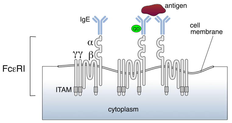
The experimental data analyzed here were part of the study described in Andrews et al. (2009). Rat mast cells (RBL-2H3) that endogenously express high levels of FcεRI were labeled with a combination of low density QD-IgE and saturating levels of “dark” IgE, both of which recognize the antigen dinitrophenyl (DNP). As a result, most of the FcεRI in the cell membrane were in IgE-FcεRI complex, but only a small percentage of the complexes were labeled with a QD (QD-IgE-FcεRI complex), such that single particle tracking density was achieved. We have previously found that the QD-IgE will bind to FcεRI on cells without inducing activation but will initiate signaling upon crosslinking (Andrews et al. 2008), demonstrating that it is a functional, monovalent reagent. A cartoon of the tetrameric IgE receptor and bound IgE or QD-IgE is given in Fig. 1. All experiments were performed at physiological temperatures (35 °C).

Fig. 1.

IgE-FcεRI and QD-IgE-FcεRI complexes. Modified image taken from Kraft and Kinet (2007)

Ten seconds after initiation of a time series, the cells were stimulated by the addition of multivalent antigen (bovine serum albumin decorated with 25 DNP, DNP-BSA) which can cross link both IgE-FcεRI or QD-IgE-FcεRI, also illustrated in Fig. 1, making them into signaling competent oligomers (Andrews 2011; Andrews et al. 2009). The QDs on the apical surface of the cells were tracked using a wide-field fluorescence microscope equipped with an electron multiplying CCD camera (Andor iXon 887) that acquired images with a frame rate of 20 frames/s for 3,000 frames, corresponding to a total time of 150 seconds. Image processing software was used to locate the center of the QDs in each of the frames. The errors in these measurements are discussed in Sect. 6.

A important difficulty in analyzing the data is that the QDs blink, that is, they emit light for some period of time, then turn off for some other period of time, repeating this cycle many times. To follow the QDs in time, individual QDs are localized in each frame and then trajectories are built based on the location of “on” QDs between frames and the diffusion coefficient (Andrews et al. 2009; Lidke et al. 2011). The results of this process is to first produce a set of segments where the QDs are on in successive frames. Then, the segments are connected based on the probability that they are from the same QD-IgE-FcεRI complex, into a path (Barroso 2011). The segments are connected based on a probability (calculated from a free diffusion model) that the same QD-IgE-FcεRI complex has moved to a new identified location while the QD was “off”. This algorithm can connect segments separated by up to 32 frames where the dot is off. This results in a data set that consists of a large number of tracks of fixed length, one track per complex, each containing a single path made up of one or more segments where the QD is on.

The data are dose-response where the dose is the concentration of stimulus added and the response is measured by tracking and then analyzing the motion of the QDs. For each data set, the cells were stimulated with six different concentrations of the multivalent antigen DNP25-BSA: 0.000; 0.001; 0.010; 0.100; 1.000 and 10 μg/ml. When the stimulus is zero, the cells are said to be unstimulated or resting. In fact, we worked with two sets of biological data, labeled A and B. We could have combined the data sets. However, independent analysis of these duplicate experiments was useful for validating our conclusions.

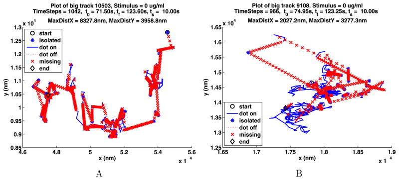
The longest path for each of the A and B data sets for unstimulated cells are shown in Fig. 2. In these figures, the start of the path is given by a black circle and the end by a black diamond. The part of the path where the QD is on is drawn as a blue solid line unless it is on for only one frame in which case it is drawn as a blue star. If two segments where the QD is on are joined by a segment of k frames where the QD is off, the end of the first segment is joined to the beginning of the second segment with a red dotted line. This line is divided into k pieces by red x’s.

Fig. 2.

The longest paths for the unstimulated data

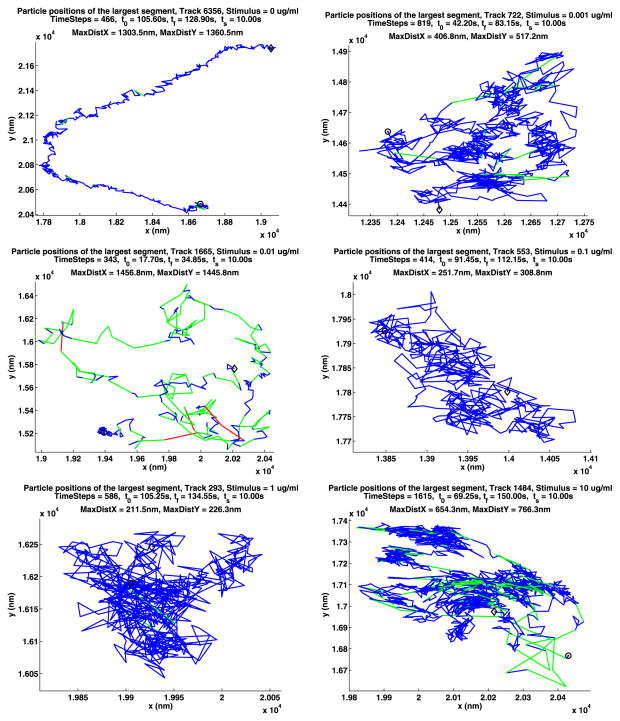
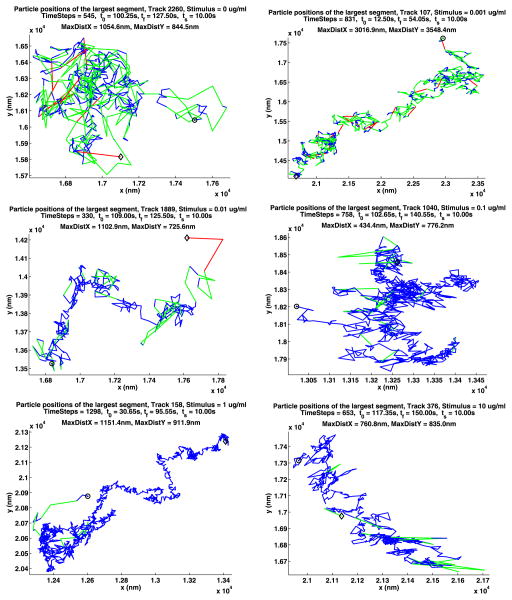
In the plot titles, the number of the track is displayed along with the concentration of stimulus used. Next, the number of time steps in the path is given along with t₀, the start time for the path, t_f, the time when the path ends, and t_s, the time when the stimulus was added. The smallest rectangle that the path will fit in has sides of length MaxDistX and MaxDistY. More path information and figures are given in Appendix A.

There is more unstimulated data because this case was both run as independent experiments as for the stimulated cells, but was also run in parallel with each of the stimulated cell experiments. From Table 1, we see that a large number of tracks were generated, resulting in a very large number of valid jumps between successive frames. This table also gives the number of cells used to generate the data. Table 2 shows that very few QDs are on in each frame of the movie. Consequently, the data in a single frame will be very noisy. Appendix B has detailed information about the statistics of the blinking. Careful time-series analysis will in some cases allow combining the data over all times. In this case, the data sets are very large so the noise in the statistical analysis will be substantially decreased.

Table 1.

The number of tracks, jumps between successive frames and cells in data sets A and B

Stimulus	A			B
	Tracks	Jumps	Cells	Tracks	Jumps	Cells
0.000	10,894	407,669	19	9,848	353,368	16
0.001	1,726	85,906	4	3,113	122,761	3
0.010	2,151	96,179	4	2,622	106,649	5
0.100	1,838	89,380	4	2,809	119,306	5
1.000	1,178	61,928	3	2,327	123,053	5
10.000	1,802	91,142	4	3,050	139,236	5

Table 2.

The minimum, mean, and maximum of the number of QDs on at each time

Stimulus	A			B
	Min	Mean	Max	Min	Mean	Max
0.000	101	136	172	81	118	162
0.001	14	29	41	24	41	60
0.010	16	32	50	17	36	52
0.100	14	30	49	21	40	58
1.000	10	21	35	22	41	62
10.000	15	30	44	29	46	54

3 Analysis Tools

The application of elementary time-series methods (Shumway and Stoffer 2006) requires the data to be ergodic and stationary. Intuitively, ergodic requires the statistics of the random variables to be independent of the spatial and temporal location. To be stationary, the mean and standard deviation of the data over a small time interval must not depend on time. We do not expect the data where the cells are stimulated to be ergodic or stationary as the state of the cell is time dependent. Additionally, the positions of the particles are not stationary because their standard deviation, which is proportional to the to the square root of the MSD, grows with time. In this situation, the standard statistical approach is to study the time series of the differenced data, which for particle tracking data is just the jumps in the positions between successive time steps, so we will focus on the jumps. The biology indicates that the data is spatially ergodic, that is, the properties of the cell membrane at different points are statistically indistinguishable. For the unstimulated cells, the time at which data is taken shouldn’t affect the data, so we model the data as being both spatially and temporally ergodic. We will not assume that the jumps are stationary, independent or identically distributed (IID). We will test the jump data for these important properties.

This discussion of the time-series analysis tools follows (Ying et al. 2009), where additional details can be found. We write the statistics that we use as expected values. It is important to know if the expected value is taken over all jumps at a given time, over all jumps in a given path followed by one particle over time, or both. We begin with a description of the time-dependent techniques applicable to the non-ergodic data from stimulated cells. We then specialize these ideas to the data from unstimulated cells where the data is modeled as ergodic. Next, we show how to apply these ideas to the data generated using QDs that blink. We finish the discussion of time series by showing these results are related to the diffusion coefficient and the MSD. Finally, we show how to estimate continuous probability distribution functions for the jumps.

Classically, the analysis of SPT data emphasized the MSD and the diffusion co-efficient. We are interested in the fine temporal and spatial scales of the motion of the QDs because we are interested in understanding the interaction of the proteins in the cell membrane with the membrane and other proteins. Time-series analysis emphasizes the use of the standard deviation or, equivalently, the variance of the jumps, which does not require averaging over time like the MSD. This analysis also emphasizes finding PDFs of the jumps, that is, the PDFs of the jump components, jump lengths and the jump angles. These PDFs contain information about the motion of the QDs at many spatial scales and the standard deviation, variance and diffusion coefficient can easily be computed from the PDF of the jump lengths.

3.1 Time-Dependent Data

The paths of the QDs are erratic, so we will model the QDs positions using vector valued random variables:

$${\overrightarrow{\mathbf{P}}}_n=({\mathbf{X}}_n,{\mathbf{Y}}_n),1\le n\le N,N>0,$$

where X_n and Y_n are real valued random variables and N and n are integers. The jumps are also random variables:

$${\overrightarrow{\mathbf{J}}}_n={\overrightarrow{\mathbf{P}}}_n-{\overrightarrow{\mathbf{P}}}_{n-1}=(\mathbf{\Delta }{\mathbf{X}}_n,\mathbf{\Delta }{\mathbf{Y}}_n),2\le n\le N.$$

In polar coordinates, the lengths of the jumps L_n and the angles Θ_n between the jump vectors and the x-axis are also random variables:

$${\mathbf{L}}_n=\left|\right|{\overrightarrow{\mathbf{J}}}_n\left|\right|=\sqrt{\mathbf{\Delta }{\mathbf{X}}_n^2+\mathbf{\Delta }{\mathbf{Y}}_n^2},{\mathbf{\Theta }}_n=arctan(\mathbf{\Delta }{\mathbf{Y}}_n,\mathbf{\Delta }{\mathbf{X}}_n),2\le n\le N,$$

where arctan gives a value in (−π, π] such that if L_n ≠ 0, then cos(Θ_n) = ΔX_n/L_n and sin(Θ_n) = ΔY_n/L_n, and consequently, tan(Θ_n) = ΔY_n/ΔX_n if ΔX_n ≠ 0. If J⃗ = (0, 0), then Θ = 0 (in Matlab).

We will express the statistics for the position and jump random variables in terms of the expected value operator E. In Sect. 3.3, we will show how to estimate the expected values from the biological data. The time-dependent mean μ and standard deviation σ of the positions are

$$\mu ({\overrightarrow{\mathbf{P}}}_n)=E({\overrightarrow{\mathbf{P}}}_n),{\sigma }^2({\overrightarrow{\mathbf{P}}}_n)=E\left(\left({\overrightarrow{\mathbf{P}}}_n-\mu ({\overrightarrow{\mathbf{P}}}_n)\right)\circ \left({\overrightarrow{\mathbf{P}}}_n-\mu ({\overrightarrow{\mathbf{P}}}_n)\right)\right),1\le n\le N,$$

while the time-dependent mean μ and standard deviation σ of the jumps are given by

$$\mu ({\overrightarrow{\mathbf{J}}}_n)=E({\overrightarrow{\mathbf{J}}}_n),{\sigma }^2({\overrightarrow{\mathbf{J}}}_n)=E\left(\left({\overrightarrow{\mathbf{J}}}_n-\mu ({\overrightarrow{\mathbf{J}}}_n)\right)\circ \left({\overrightarrow{\mathbf{J}}}_n-\mu ({\overrightarrow{\mathbf{J}}}_n)\right)\right),2\le n\le N.$$ (1)

The means and standard deviations of other random variables have similar expressions.

The time-dependent MSD is given by

$${\text{MSD}}_{n,k}=E\left(({\overrightarrow{\mathbf{P}}}_{n+k}-{\overrightarrow{\mathbf{P}}}_n)\circ ({\overrightarrow{\mathbf{P}}}_{n+k}-{\overrightarrow{\mathbf{P}}}_n)\right),1\le k\ll N,1\le n\le N-k,$$

that is, writing P⃗_n+k − P⃗_n as a telescoping sum,

$${\text{MSD}}_{n,k}=E\left(\sum _{j=1}^k{\overrightarrow{\mathbf{J}}}_{n+j}\circ \sum _{j=1}^k{\overrightarrow{\mathbf{J}}}_{n+j}\right),1\le k\ll N,1\le n\le N-k.$$

If the J⃗_n are independent and mean zero, then

$${\text{MSD}}_{n,k}=\sum _{j=1}^{k}E({\overrightarrow{\mathbf{J}}}_{n+j}\circ {\overrightarrow{\mathbf{J}}}_{n+j}),1\le k\ll N,1\le n\le N-k.$$ (2)

The moments of the jump lengths L_n,

$$M_n^{(k)}=E\left({\mathbf{L}}_n^k\right),0\le k\le N,2\le n\le N,$$

are used in our analysis.

If

$${\stackrel{\sim }{\rho }}_{n,k}=E({\overrightarrow{\mathbf{J}}}_n\circ {\overrightarrow{\mathbf{J}}}_{n-k}),0\le k\ll N,k+2\le n\le N,$$

then the autocorrelation coefficients for the jumps are

$${\rho }_{n,k}=\frac{{\stackrel{\sim }{\rho }}_{n,k}}{{\stackrel{\sim }{\rho }}_{n,0}},0\le k\ll N,k+2\le n\le N,$$ (3)

if ρ̃_n,0 ≠ 0. The random variables J⃗_n and J⃗_n−k are independent if and only if ρ_n,k = 0.

3.2 Ergodic in Time Data

We now assume that the jumps are time independent, that is, they are independent and identically distributed (IID). In this case, the random variables J⃗_n, ΔX_n, ΔY_n, L_n and Θ_n are all independent copies of a single random variable J⃗, ΔX, ΔY, L and Θ. We will also assume that J⃗, ΔX, ΔY are mean zero and have standard deviations σ_r, σ_x and σ_y, respectively. We also assume that ΔX and ΔY are independent so that

$${\sigma }_r^2={\sigma }_x^2+{\sigma }_y^2.$$

Thus,

$$\begin{array}{l}\mu ({\overrightarrow{\mathbf{J}}}_n)=E({\overrightarrow{\mathbf{J}}}_n)=E(\overrightarrow{\mathbf{J}})=\mu (\overrightarrow{\mathbf{J}})=0\\ {\sigma }^2({\overrightarrow{\mathbf{J}}}_n)=E({\overrightarrow{\mathbf{J}}}_n\circ {\overrightarrow{\mathbf{J}}}_n)=E(\overrightarrow{\mathbf{J}}\circ \overrightarrow{\mathbf{J}})={\sigma }^2(\overrightarrow{\mathbf{J}})={\sigma }_r^2,2\le n\le N.\end{array}$$

From (2), the MSD is

$${\text{MSD}}_k=kE(\overrightarrow{\mathbf{J}}\circ \overrightarrow{\mathbf{J}})=k{\sigma }^2(\overrightarrow{\mathbf{J}}),k\ge 1.$$ (4)

The second moments of the jump lengths satisfy

$$M^{(2)}=M_n^{(2)}=E({\mathbf{L}}_n^2)=E({\overrightarrow{\mathbf{J}}}_n\circ {\overrightarrow{\mathbf{J}}}_n)={\sigma }^2({\overrightarrow{\mathbf{J}}}_n)={\sigma }^2(\overrightarrow{\mathbf{J}})={\sigma }_r^2,2\le n\le N.$$

An important null hypothesis is that the coordinates of the jumps, ΔX and ΔY, are independent of each other and each is IID and normally distributed with mean zero and standard deviation scale parameter s. Equivalently, L and Θ are independent, with Θ uniformly distributed in [−π, π], and L has the probability distribution w(r, s) = w(r/s)/s where

$$w(r)={re}^{-\frac{r^2}{2}}.$$

The PDF w(r, s) is a special case of the general chi distribution with scale parameter s or the general Weibull distribution with shape parameter 2 and scale parameter $\sqrt{2}s$. We will call this distribution the simple chi or simple Weibull distribution. The moments of this distribution are

$$M^{(1)}=\sqrt{\frac{\pi }{2}}s,M^{(2)}=2s^2={\sigma }_r^2.$$

Because of the complexity of the cell membrane, we do not expect the data to satisfy the null hypothesis, but the deviation of the statistics for the biological data from the null hypothesis will provide insight into the nature of the motion of the receptors.

3.3 Time Series with Blinking

The estimation of the statistics related to the random variables in our model is made more complicated by the time dependence of the statistics and by the missing data due to the blinking of the QDs. Generally, all analysis concepts are the same as in the non-blinking case, except when the QD is off, computations are skipped.

A data set will contain M > 0 tracks described by

$$x_{m,n},y_{m,n},v_{m,n},1\le m\le M,1\le n\le N.$$

The vectors

$${\overrightarrow{r}}_{m,n}=(x_{m,n},y_{m,n})$$

estimate the position of the QDs. If v_m,n = 1, then the QD is on and the position of the QD is valid data, while if v_m,n = 0, the QD is off. Even when the QD is off, we assume that x_n and y_n are finite numbers. Each track contains only one path. For a fixed track m, if n_start is the first value of n where v_m,n = 1 and n_end is the largest value of n where v_m,n = 1, then a path is given by the points satisfying

$$n_{\text{start}}\le n\le n_{\text{end}},$$

as shown in Fig. 2, where

$$t_0=n_{\text{start}}/20,t_f=n_{\text{end}}/20,$$

because there are 20 frames per second.

We first give some definitions that apply to data from both resting cells and stimulated cells. As noted before, because the data from the stimulated cells is not ergodic, the statistics for these data will depend on the time step n or equivalently on the time t. Because of the blinking, we will need to count the valid data as we compute statistics. We do this by introducing a modified definition of the expected value operator that averages only over valid data. For example, if we set

$$v_n=\sum _{m=1}^M{v}_{m,n},$$

which is the number of valid points at time n, then the time-dependent means of the position vectors are

$$\mu ({\overrightarrow{\mathbf{P}}}_n)=E({\overrightarrow{\mathbf{P}}}_n)\approx \frac{1}{v_n}\sum _{m=1}^M{v}_{m,n}{\overrightarrow{r}}_{m,n}\text{if}{v}_n\ne 0.$$ (5)

and the time-dependent standard deviations of the position vectors are

$$\begin{array}{l}{\sigma }^2({\overrightarrow{\mathbf{P}}}_n)=E\left(\left({\overrightarrow{\mathbf{P}}}_n-\mu ({\overrightarrow{\mathbf{P}}}_n)\right)\circ \left({\overrightarrow{\mathbf{P}}}_n-\mu ({\overrightarrow{\mathbf{P}}}_n)\right)\right)\\ \approx \frac{1}{v_n}\sum _{m=1}^M{v}_{m,n}\left({\overrightarrow{r}}_{m,n}-\mu ({\overrightarrow{\mathbf{P}}}_n)\right)\circ \left({\overrightarrow{r}}_{m,n}-\mu ({\overrightarrow{\mathbf{P}}}_n)\right)\text{if}{v}_n\ne 0.\end{array}$$

In this section, expected values are undefined (not valid) if they are taken over an empty set of data, that is, when the divisor in the expected value is zero. Also, because of the blinking, v_n is typically small.

The jumps in the tracks are

$$\mathrm{\Delta }{\overrightarrow{r}}_{m,n}=(\mathrm{\Delta }{x}_{m,n},\mathrm{\Delta }{y}_{m,n})=(x_{m,n}-x_{m,n-1},y_{m,n}-y_{m,n-1}),1\le m\le M,2\le n\le N.$$

The jump data is valid if v_m,n = v_m,n−1 = 1 or if V_m,n = 1 where

$$V_{m,n}=v_{m,n}{v}_{m,n-1},1\le m\le M,2\le n\le N.$$ (6)

A cautionary note: all tracks must contain at least one valid position. However, it is possible (but not very likely) that a track does not have any valid jumps. In this case, for a fixed m, V_m,n = 0 for all n. It is also possible, and more likely, that for fixed n, V_m,n = 0 for all m.

If

$$V_n=\sum _{m=1}^M{V}_{m,n},2\le n\le N,$$ (7)

that is, the number of valid jumps at time n, then the means of the jumps are estimated using

$$\mu ({\overrightarrow{\mathbf{J}}}_n)=E({\overrightarrow{\mathbf{J}}}_n)\approx \frac{1}{V_n}\sum _{m=1}^M{V}_{m,n}\mathrm{\Delta }{\overrightarrow{r}}_{m,n}\text{if}{V}_n\ne 0,$$ (8)

while the standard deviations of the jumps are estimated by

$$\begin{array}{l}{\sigma }^2({\overrightarrow{\mathbf{J}}}_n)=E\left(\left({\overrightarrow{\mathbf{J}}}_n-\mu ({\overrightarrow{\mathbf{J}}}_n)\right)\circ \left({\overrightarrow{\mathbf{J}}}_n-\mu ({\overrightarrow{\mathbf{J}}}_n)\right)\right)\\ \approx \frac{1}{V_n}\sum _{m=1}^M{V}_{m,n}\left(\left(\mathrm{\Delta }{\overrightarrow{r}}_{m,n}-\mu ({\overrightarrow{\mathbf{J}}}_n)\right)\circ \left(\mathrm{\Delta }{\overrightarrow{r}}_{m,n}-\mu ({\overrightarrow{\mathbf{J}}}_n)\right)\right),\text{if}{V}_n\ne 0.\end{array}$$ (9)

Also, the lengths of the jumps and the angles between the jumps and the x-axis are

$$L_{m,n}=\sqrt{\mathrm{\Delta }{x}_{m,n}^2+\mathrm{\Delta }{y}_{m,n}^2},{\theta }_{m,n}=arctan(\mathrm{\Delta }{y}_{m,n},\mathrm{\Delta }{x}_{m,n}),$$

for 1 ≤ m ≤ M and 2 ≤ n ≤ N. All of the moments of the jump sizes are estimated using

$$M_n^{(k)}\approx \frac{1}{V_n}\sum _{m=1}^M{V}_{m,n}{L}_{m,n}^k,k\ge 0,2\le n\le N.$$

To estimate the time-dependent autocorrelation coefficients (3), we need to compute J⃗_n ∘ J⃗_n−k. We can do this when V_m,n and V_m,n−k are valid jumps (6), but prefer to make the more restrictive requirement that all of the V_m,n−i are valid jumps for 0 ≤ i ≤ k:

$$Q_{m,n,k}=V_{m,n}\ast V_{m,n-1}\ast \cdots \ast V_{m,n-k},0\le k\ll N,k+2\le n\le N,1\le m\le M,$$

and then set

$$Q_{n,k}=\sum _{m=1}^M{Q}_{m,n,k}.$$

If

$${\stackrel{\sim }{\rho }}_{n,k}=\frac{1}{Q_{n,k}}\sum _{m=1}^M{Q}_{m,n,k}(\mathrm{\Delta }{\overrightarrow{r}}_{m,n}\circ \mathrm{\Delta }{\overrightarrow{r}}_{m,n-k}),\text{if}{Q}_{n,k}\ne 0,$$

then the estimate of the time-dependent autocorrelation coefficient is

$${\rho }_{n,k}=\frac{{\stackrel{\sim }{\rho }}_{n,k}}{{\stackrel{\sim }{\rho }}_{n,0}},$$ (10)

if ρ̃_n,0 ≠ 0.

3.4 Ergodic and Stationary Data

If the jump data is also ergodic in time and stationary, then we can also take expected values over time. So, using (7), define

$$V=\sum _{n=2}^N{V}_n=\sum _{n=2}^N\sum _{m=1}^M{V}_{m,n},$$

and then as in (8), define

$$\overrightarrow{\mu }=\mu (\overrightarrow{\mathbf{J}})=E(\overrightarrow{\mathbf{J}})\approx \frac{1}{V}\sum _{n=2}^N\sum _{m=1}^M{V}_{m,n}\mathrm{\Delta }{\overrightarrow{r}}_{m,n}\text{if}V\ne 0.$$ (11)

For the standard deviation, as in (9) replacing μ(J⃗_n) by μ(J⃗), define

$$\begin{array}{l}{\sigma }_r^2={\sigma }^2(\overrightarrow{\mathbf{J}})=E\left(\left(\overrightarrow{\mathbf{J}}-\mu (\overrightarrow{\mathbf{J}})\right)\circ \left(\overrightarrow{\mathbf{J}}-\mu (\overrightarrow{\mathbf{J}})\right)\right)\\ \approx \frac{1}{V}\sum _{n=2}^N\sum _{m=1}^M{V}_{m,n}\left(\left(\mathrm{\Delta }{\overrightarrow{r}}_{m,n}-\mu (\overrightarrow{\mathbf{J}})\right)\circ \left(\mathrm{\Delta }{\overrightarrow{r}}_{m,n}-\mu (\overrightarrow{\mathbf{J}})\right)\right),\text{if}V\ne 0.\end{array}$$ (12)

If J⃗ is mean zero, then

$${\sigma }_r^2={\sigma }^2(\overrightarrow{\mathbf{J}})=E(\overrightarrow{\mathbf{J}}\circ \overrightarrow{\mathbf{J}})\approx \frac{1}{V}\sum _{n=2}^N\sum _{m=1}^M{V}_{m,n}(\mathrm{\Delta }{\overrightarrow{r}}_{m,n}\circ \mathrm{\Delta }{\overrightarrow{r}}_{m,n}),\text{if}V\ne 0.$$ (13)

The moments of L are estimated by

$$M^{(k)}=E({\mathbf{L}}^k)\approx \frac{1}{V}\sum _{n=2}^N\sum _{m=1}^M{V}_{m,n}{\left|\right|\mathrm{\Delta }{\overrightarrow{r}}_{m,n}\left|\right|}^k,\text{if}V\ne 0.$$

Note that

$$M^{(2)}={\sigma }_r^2.$$

To define the time-independent autocorrelation coefficients, let

$$Q_k=\sum _{n=k+2}^N{Q}_{n,k}=\sum _{n=k+2}^N\sum _{m=1}^M{Q}_{m,n,k},$$

and then, using (10), set

$${\stackrel{\sim }{\rho }}_k=\frac{1}{Q_k}\sum _{n=k+2}^N\sum _{m=1}^M{Q}_{m,n,k}(\mathrm{\Delta }{\overrightarrow{r}}_{m,n}\circ \mathrm{\Delta }{\overrightarrow{r}}_{m,n-k}),\text{if}{Q}_k\ne 0.$$

Finally,

$${\rho }_k=\frac{{\stackrel{\sim }{\rho }}_k}{{\stackrel{\sim }{\rho }}_0},$$ (14)

if ρ̃₀ ≠ 0.

3.5 The Diffusion Coefficient

For mean zero IID J⃗_n, the MSD (4) is given by

$${\text{MSD}}_k={kM}^{(2)}=k{\sigma }_r^2.$$

It is known that in two dimensions

$$\text{MSD}(t)=4Dt,$$

where D is the diffusion coefficient. If the time step in the random walk is Δt and t = k Δt, then

$$4Dt=\text{MSD}(t)={\text{MSD}}_k=M^{(2)}k=\frac{M^{(2)}}{\mathrm{\Delta }t}t.$$

Consequently, the diffusion coefficient is given by

$$D=\frac{M^{(2)}}{4\mathrm{\Delta }t}=\frac{{\sigma }_r^2}{4\mathrm{\Delta }t}.$$ (15)

If the components of the jumps are independent, then

$${\sigma }_r^2={\sigma }_x^2+{\sigma }_y^2.$$

In the case that the components of the jumps are normally distributed with mean zero and standard deviation s, then σ_x = σ_y = s and

$${\sigma }_r^2=2s^2.$$

Equivalently the length of the jumps have a simple chi distribution with second moment M⁽²⁾ = 2s² and the jump angles are uniformly distributed. Then,

$$D=\frac{s^2}{2\mathrm{\Delta }t}.$$ (16)

For the stimulated data, we define the time-dependent diffusion coefficient using (1):

$$D_n=\frac{{\sigma }^2({\overrightarrow{\mathbf{J}}}_n)}{4\mathrm{\Delta }t}.$$

This time-dependent diffusion coefficient does not depend on how the segments are connected to make a path.

3.6 Estimating Probability Distribution Functions

Even though we are using vector valued random variables, we will only compute PDFs for scalar valued random variables, so let y_j, 1 ≤ j ≤ J, J ≫ 1 be real numbers. Choose a number a so all (or maybe almost all) of the y_j satisfy −a ≤ y_j ≤ a. We will then divide the interval [−a, a] into 2I + 1 intervals of length Δx = 2a/(2I + 1). The centers of the intervals are then given by

$$x_i=i\mathrm{\Delta }x,-I\le i\le I,$$

and the intervals, called bins, are given by

$$I_i=\left[(i-1/2)\mathrm{\Delta }x,(i+1/2)\mathrm{\Delta }x\right],-I\le i\le I.$$

Now let K_i be the number of data points y_j ∈ I_i and then set

$$K=\sum _{i=-I}^I{K}_i,p_i=\frac{K_i}{K\mathrm{\Delta }x},-I\le i\le I.$$ (17)

The p_i give an approximation to a continuous probability distribution in the sense that

$$\sum _{-I}^I{p}_i\mathrm{\Delta }x=1.$$

The mean and standard deviation of the data can be estimated using

$$\mu =M^{(1)}=\sum _{-I}^I{x}_i{p}_i\mathrm{\Delta }x,M^{(2)}=\sum _{-I}^I{x}_i^2{p}_i\mathrm{\Delta }x,{\sigma }^2=M^{(2)}-{\mu }^2.$$ (18)

4 Analysis of the Data from Unstimulated Cells

In this section we use time-series analysis to better understand the data from unstimulated cells. We begin by using the time-dependent means and standard deviations of the jumps in position of successive time steps to support modeling the data as ergodic and stationary. Next, we compute the autocorrelation coefficients and show that the jumps at different times can be modeled as independent. With this in place, it is reasonable to use all of the jumps at all times to estimate the mean and standard deviation of the jumps. The means of all of the jumps are near zero, supporting modeling the jumps as mean zero. The standard deviations of all of the jumps for data sets A and B are similar, supporting modeling the jumps as identically distributed. Consequently, we model the jumps as mean zero and IID and proceed with analyzing the probability distribution functions for the jump components, jump lengths and jump angles. Because we have two data sets generated by independent experiments, this analysis also supports modeling the jumps as identically distributed.

An important result is that the components of the jumps are not normally distributed, as should be expected as the cell membrane is a complex medium. However, the angles of jumps are uniformly distributed, as also should be expected as there is no preferred direction in the cell membrane. Consequently, the PDF of the jump sizes contain all of the information about the failure of the components of jumps to satisfy the null hypothesis of being normally distributed, so we emphasize the analysis of the distribution of the jump sizes.

A minor point is that during this analysis we found that the path-constructing algorithms were producing a very small percentage of anomalous jumps with sizes larger that 346 nm. This accounts for less than 1/2 percent of the data, consequently we eliminated these jumps from the analysis; see Appendix C. The path-constructing algorithms are being improved, but any improvements should not significantly affect our results.

4.1 Preliminary Analysis

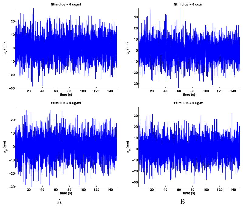
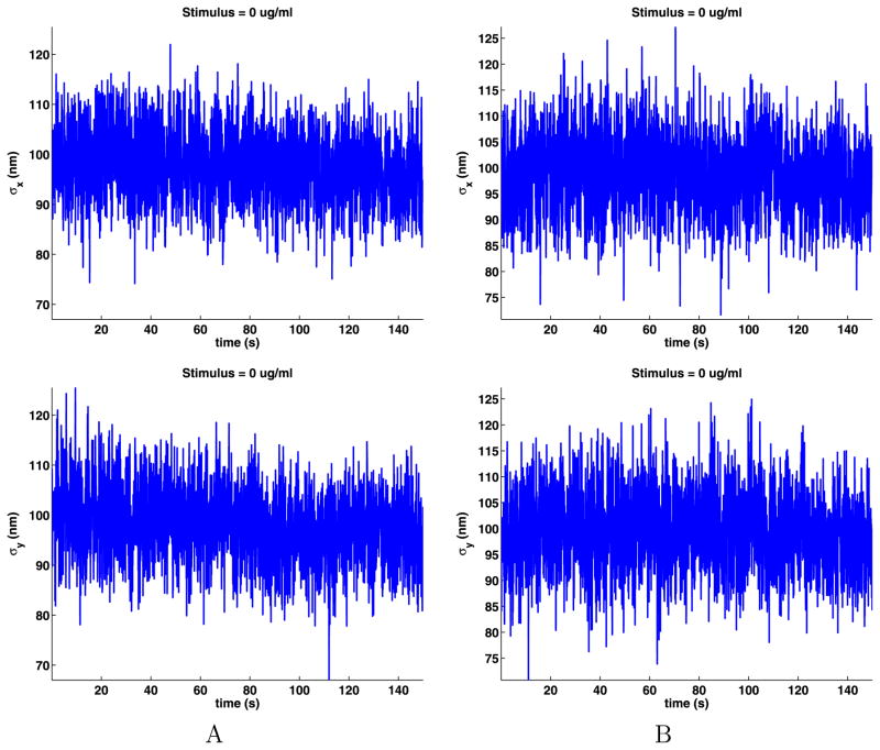
As noted before, we assume that the data for any cell are spatially ergodic as there are no special locations on the cell membrane. The time-dependent means (8) and standard deviations (9) of the jumps are shown in Figs. 3 and 4. These plots are noisy because only a few QDs are on at any given time (see Appendix B), but still, we can see that the data sets do not have a noticeable trend, supporting modeling the data as time ergodic and stationary.

Fig. 3.

Time-dependent means of the jump components

Fig. 4.

Time-dependent standard deviations of the jump components

We estimated the mean μ⃗ (11) and standard deviation σ_r (12) of the jumps and record these in Table 3. Note that μ⃗ is listed componentwise, while σ_r refers to the length of the jumps. We use the dimensionless parameter ||μ⃗||/σ_r to estimate the size of the mean, which is close to zero. The fact that the standard deviations for data sets A and B are close to the same, supports modeling the jumps as identically distributed.

Table 3.

Number of jumps N, mean μ⃗, standard deviation σ_r and mean zero test ||μ⃗||/σ_r for the jumps

	N	μ⃗	σr	||μ⃗||/σr
A	405,600	(0.2713, −0.1351)	138.0	0.0023
B	351,700	(−0.1184, 0.0631)	139.5	0.0009

To test if the jump components computed from the unstimulated data are independent, we computed their autocorrelation coefficients for 0 ≤ k ≤ 5 and display them in Table 4. To understand the significance of these coefficients, we computed the autocorrelation coefficients for simulated IID normally distributed random jumps with mean and standard deviation of the full data set. Here, it is important to take into account the blinking of the QDs, so for the generated data, the autocorrelation coefficients were computed using the same valid positions as the biological data. The results were averaged over 100 simulations. The autocorrelations for the biological data are larger than for the simulated random data, but are still sufficiently small that we will model them as zero, that is, we model the jumps as independent. Putting all of this together, we will model the unstimulated data assuming the jumps are ergodic in space and time, stationary, mean zero and IID. A natural next step is to analyze the probability distribution functions for the jump components, the jump lengths and the jump angles.

Table 4.

Autocorrelation coefficients of the jumps and their corresponding coefficients for computer generated random jumps

k	0	1	2	3	4	5
A	1.0000	0.0848	−0.0483	−0.0239	−0.0157	−0.0076
Random	1.0000	−0.0000	−0.0003	−0.0017	−0.0020	−0.0031
B	1.0000	0.0767	−0.0503	−0.0261	−0.0146	−0.0102
Random	1.0000	−0.0000	−0.0007	0.0012	−0.0001	0.0009

4.2 Analyzing the Distribution of the Jump Components

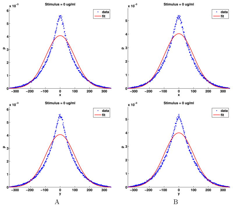
We will compute the PDFs of the jump components using the results in Sect. 3.6 and then check to see if the PDFs are normally distributed. We put the data into 500 bins (17), displaying the results in Fig. 5. We used the PDFs to compute the mean and standard deviation of the jumps using (18), which agree with the values given in Table 3. Next, we used the standard deviations to determine a mean zero normal distribution that best fits the biological data and plotted these in Fig. 5. Clearly the distribution of the jump components are not normally distributed. However, these distributions are very similar for both components and for data sets A and B, supporting modeling the jump data using identically distributed random variables.

Fig. 5.

Distributions of the jump components and their normal fits

More importantly, from Fig. 5 we see that for the x and y jump components, there is an excess of short jumps. More precisely, for |x|, |y| < 50 nm, short jumps are in excess of what would be expected for a normal distribution. For approximately 50 < |x|, |y| < 190 nm, there are fewer jumps than in a normal distribution. A simple explanation for the excess short jumps is that there are barriers to longer jumps in the cell membrane and the scale of some of these barriers is less than 50 nm for the jump components or 70 nm for the jump lengths. Most importantly, the fact that the PDFs for the data are smooth implies there are significant barriers to the diffusion of receptors for every length scale.

To test if the components of jumps are normally distributed, we use the two-sample Kolmogorov–Smirnov goodness-of-fit hypothesis test (kstest2 in the Matlab statistics toolbox). The null hypothesis is that the jump components come from a normal distribution. We use a stringent significance level α = 0.0001. The p-values for data set A and B for both the x and y jump components are 0.000. The decision to reject the null hypothesis occurs when the significance level α = 0.0001 equals or exceeds the p-value. As indicated by Fig. 5, this is a strong rejection of the null hypothesis, so the x and y jump components will not be modeled as normally distributed.

4.3 Analyzing the Distribution of the Angles and Jump Lengths

For IID random walks, the jump components are normally distributed if and only if the jump angles are uniformly distributed, and the jump lengths have a simple chi distribution (Ying et al. 2009), which is the same as the simple Weibull distribution. The previous discussion shows that the components of the jumps are not normally distributed. Thus it cannot be the case that both the jump angles are uniformly distributed and the jump lengths have a simple chi distribution. Intuitively, we expect that the jump angles to be uniformly distributed because at a point in the cell membrane there is no preferred direction.

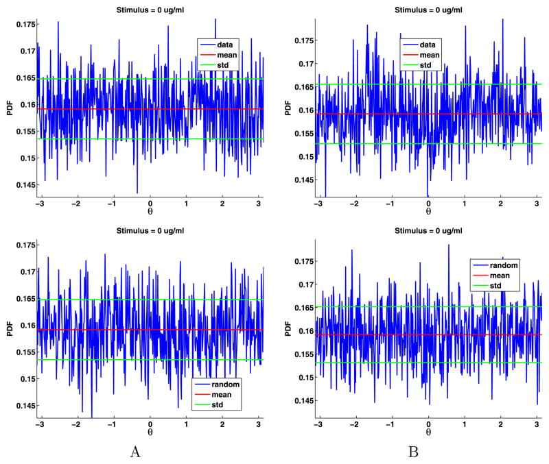
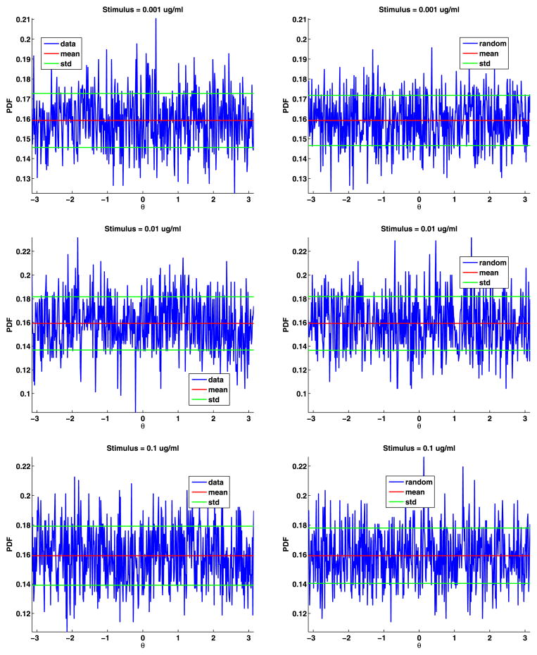
To estimate the distribution of the angles, we divided [−π, π] into 500 bins and then binned the angles and computed their PDF (see Fig. 6). The angles are uniformly distributed; their PDF is θ = π/2 = 0.1592. For both data sets, the mean of the angles differs from π/2 by less than 0.0001. We also generated the same number of angles as in the data, binned the results, and plotted these PDFs (again, see Fig. 6). These plots are very similar to the plots of the data. We also plot the mean and standard deviation of the angles to help in comparing the plots. To test if the angles are uniformly distributed, we again used the two-sample Kolmogorov–Smirnov goodness-of-fit hypothesis test with a significance level α = 0.0001. The null hypothesis is that these angles come from a uniform distribution. The p-value for data set A is 0.8567, and for data set B is 0.7614. The rejection of the null hypothesis occurs when the significance level α equals or exceeds the p-value, so we cannot reject the null hypothesis. The magnitude of the p-values strongly supports the modeling of the jump angles with a uniform distribution.

Fig. 6.

Data angles (top) and generated random angles (bottom) for data sets A and B

Now that we know that the jumps cannot have a simple chi or Weibull PDF, we will check if the PDFs of the data are given by any of three other distributions (Ying et al. 2009). The general chi PDF with d degrees of freedom and scale factor s is c(r, s, d) = c(r/s, d)/s where

$$c(r,d)=\frac{2}{2^{d/2}\mathrm{\Gamma }(d/2)}{r}^{d-1}{e}^{-\frac{r^2}{2}},$$ (19)

r ≥ 0, s > 0, d ≥ 1, and the gamma function satisfies Γ(n) = (n − 1)! when n is an integer. The general Weibull PDF is w(r, s, k) = w(r/s, k)/s where

$$w(r,k)={kr}^{k-1}{e}^{-r^k},$$ (20)

where r > 0, s > 0 and k > 0. The simple chi distribution is given by d = 2 and the simple Weibull is given by k = 2 in which case $s=\sqrt{2}{\sigma }_r$. The power-law distribution was devised in Ying et al. (2009) where it was called the long-short distribution. It is designed to test for power laws for both small and large r. It is given by p(r, s, α, β) = p(r/s, α, β)/s, where

$$p(r,\alpha ,\beta )=\frac{\alpha (\beta -1)r^{\alpha -1}}{{(1+r^{\alpha })}^{\beta }},$$ (21)

r ≥ 0, s > 0, α > 0 and β > 1.

The second moments of these distributions are

$$M_c^{(2)}=s^{2}d,M_w^{(2)}=s^2\mathrm{\Gamma }\left(1+\frac{2}{k}\right),$$ (22)

and

$$M_p^{(2)}=s^2\frac{\mathrm{\Gamma }(1+\frac{2}{\alpha })\mathrm{\Gamma }(\beta -\frac{2}{\alpha }-1)}{\mathrm{\Gamma }(\beta -1)},\alpha (\beta -1)-2>0.$$ (23)

All of these formulas over estimate

$${\sigma }_r\approx \sqrt{M^{(2)}},$$

because there are very long jumps in the data.

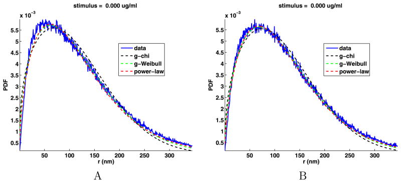
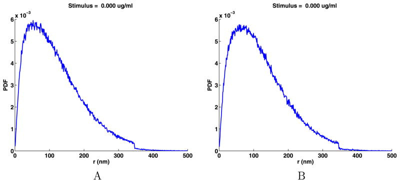
The parameters for the fits along with the mean square relative error for the fits are given in Table 5. The relative errors are all less than one percent, so the fits are very good. We plot the jump lengths PDFs along with the three fits in Fig. 7. From this figure, we see that all fits underestimate the number of jumps near r = 50 nm. For r large, the chi and Weibull distributions decay exponentially, but the chi decays faster than the Weibull. Both underestimate the number of longer jumps with the Weibull being better than the chi. The power law provides the best estimates for the larger jump sizes. The decay for large r of the power-law distribution is of the form

Table 5.

General chi, general Weibull, and power-law fit parameters to the PDF of the jump lengths, and their relative mean square errors (e)

	General chi			General Weibull			Power law
	d	s	e	k	s	e	α	β	s	e
A	1.35	116.79	0.0086	1.49	130.39	0.0035	1.54	9.78	561.02	0.0031
B	1.41	116.37	0.0056	1.55	133.70	0.0022	1.59	14.10	663.27	0.0020

Fig. 7.

Jump lengths PDFs with the general chi, general Weibull and power-law fits

$$p\approx {Cr}^{-\gamma },\gamma =\alpha (\beta -1)+1.$$ (24)

For data set A, γ = 14.521 and for data set B, γ = 21.829, so the decay of the long jumps is quite rapid.

All these distributions with d = k = α have the same power law near r = 0:

$$p\approx {Cr}^{d-1}.$$

More precisely, we used the Matlab function rat to find the closest rational approximate of d, k, and α with a denominator less than 10. The chi distribution for data set A gives 4/3; all others give 3/2. The fact that d is less than to 2 indicates that the PDF of the jump lengths are not close to normally distributed. It is interesting that the estimates of d are so consistent for the different distributions, indicating that this behavior is very robust.

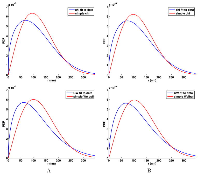
To better understand the consequence of d being less than 2, we compare the general chi and Weibull distributions for the data to the theoretical distribution for IID jumps that are normally distributed. We use (22) to compute $M_c^{(2)}$ for the data using the values of s and d that are given in Table 5. Then we use

$$d=2,s=\sqrt{\frac{M_c^{(2)}}{d}},$$

to compute the distribution expected in the case of normal diffusion. The plots of the distributions given in Fig. 8 clearly indicate that there are excessive short jumps for small r. We now repeat this for the Weibull distribution using (22) to compute $M_w^{(2)}$ for the data using the values of s and k that are given in Table 5. Then we use

Fig. 8.

In the top row, comparison of the simple chi and general chi distributions that have the same second moment as the data, and in the bottom row, comparison of the simple Weibull and general Weibull distributions that have the same second moment as the data

$$d=2,s=\sqrt{\frac{M_w^{(2)}}{\mathrm{\Gamma }(1+\frac{2}{k})}},$$

to compute the distribution expected in the case of normal diffusion. Again, the plots of the distributions given in Fig. 8 clearly indicate that there are excessive short jumps for small r.

Another way to quantify the excess short jumps is to use the first point where the two PDF curves in Fig. 8 cross which we give in Table 6. We can also use the curves for the jump components shown in Fig. 5. For both the A and B data sets, we estimate the crossing points as x_c = 50 nm and y_c = 50 nm and then set

Table 6.

Estimates of the point with the smallest r where the normal and general chi and Weibull distributions curves cross

	Chi	Weibull	rc
A	64 nm	75 nm	70 nm
B	64 nm	77 nm	70 nm

$$r_c=\sqrt{x_c^2+y_c^2}\approx 70\text{nm}.$$ (25)

All of these estimates say that there is a significant excess of jumps substantially shorter than 70 nm. It is reasonable to attribute this excess of small jumps to obstructions to the motion of the receptors on the tens of nanometer scale. Moreover, for IID random walks in spaces of dimension d that have normally distributed jumps, the distribution of the jump sizes is given by c(r, s, d), so d gives an estimate of the dimension of the space in which the diffusion is occurring. In three dimensions, this is the well-known Maxwell–Boltzmann distribution. It appears as if the cell membrane has dimension d < 2, which is really a measure of how much the jump lengths are reduced from normal diffusion in the cell membrane (Ying et al. 2009). We can also interpret this result to mean that the diffusion is in a fractal space of dimension approximately d. In Ying et al. (2009), the data sets are much smaller, so the results are much noisier, but still d was found to be smaller than two.

4.4 Summary

This section began by showing that it is reasonable to model the jump data from un-stimulated cells as ergodic, stationary, independent, identically distributed and mean zero. Consequently, the data can be studied using standard time-series analysis. The fitting of the distributions of the jump components shows that there is an excess of short jumps. We also show that the jump angles can be modeled as uniformly distributed, but that the jump lengths cannot be modeled by a simple chi distribution. However, the jump lengths distribution can be fit with a general chi, general Weibull or a power law. All of these fits show that, for small r, the distribution behaves like r^d−1 where d < 2, which implies there is an excess of short jumps as compared to normally distributed jumps. The fit by the chi distribution suggest that the motion of the QDs can be modeled as diffusion in a fractal space of dimension d. Finally, we compared the general chi and general Weibull fits to simple chi and simple Weibull distributions with the same standard deviation to see that there are substantial barriers to free diffusion well below the 70 nm scale. For jumps of intermediate size, the power-law distribution gives the best fit and estimates that the power-law decay is fast. Other authors have fit jump data with a weighted average of several Gaussians (Kubitscheck 2009), but this would not capture the power-law behavior.

These results have significant implications for biologists studying membrane dynamics and heterogeneity. Current models suggest that the movement of proteins in membranes is confined by interactions with membrane structures such as lipid rafts, protein islands and cytoskeletal corrals (Pike 2006; Lillemeier et al. 2006; Kusumi et al. 2005; Lidke and Wilson 2009). Previous analysis of similar data sets to those studied here provided clear evidence for the existence of micron-scale cytoskeletal corrals that form large confinement zones for QD-IgE-FcεRI complexes (Andrews et al. 2008, 2009; Andrews 2011). Our more detailed analysis establishes the presence of additional confinement zones on the order of tens of nanometers within the actin-defined corrals. Previous high-resolution electron microscopy (EM) showed that receptors are distributed in clusters across the membrane (Andrews 2011; Wilson et al. 2002; Seagrave et al. 1991). The nanometer-scale clusters seen previously by EM are very likely a freeze-frame representation of membrane microdomain organization now revealed by live cell single particle tracking. This connection is even clearer using a new method of analyzing clustering (Espinoza et al. 2012) that emphasizes compact clusters.

An even more important point is that the PDFs for the jump components and the jump lengths are smooth, that is, there are no special features at any length, implying that there are barriers at all scales. It would seem that the rafts, island and corrals do not cause diffusion to slow at any dominant length scale, implying that these structures have a wide range of sizes.

5 Analysis of the Data from Stimulated Cells

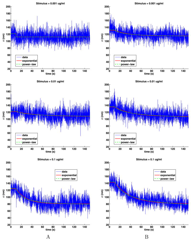
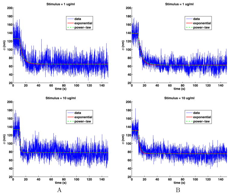
Plots of the time-dependent standard deviation of the jumps presented in Fig. 9 show that the motion of the QDs in stimulated cells can be broken into three parts: the same as in unstimulated cells until the stimulus is added at 10 seconds; a slowing of the motion that is highly stimulus dependent; and then a long period of slower motion in the tail. The plots also include some fits to the data that will be explained below. A striking feature of the plots is that they are noisy as a function of time. This is because, at any given time, there are approximately 30 QDs on (see Table 2), which is a small data set. As we analyze the data, we will see that we should divide the data into two cases: weak stimuli (0.001, 0.01) and strong stimuli (0.1, 1, 10). Because of the simple relationship (15) between the diffusion coefficient and the standard deviation of the jump sizes, these plots are essentially the same as those in Lidke et al. (2007), Andrews et al. (2008, 2009), Andrews (2011). As before, we removed jumps larger than 346 nm from the analysis.

Fig. 9.

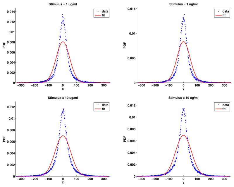
Time-dependent standard deviations of the jump lengths and their exponential and power-law fits

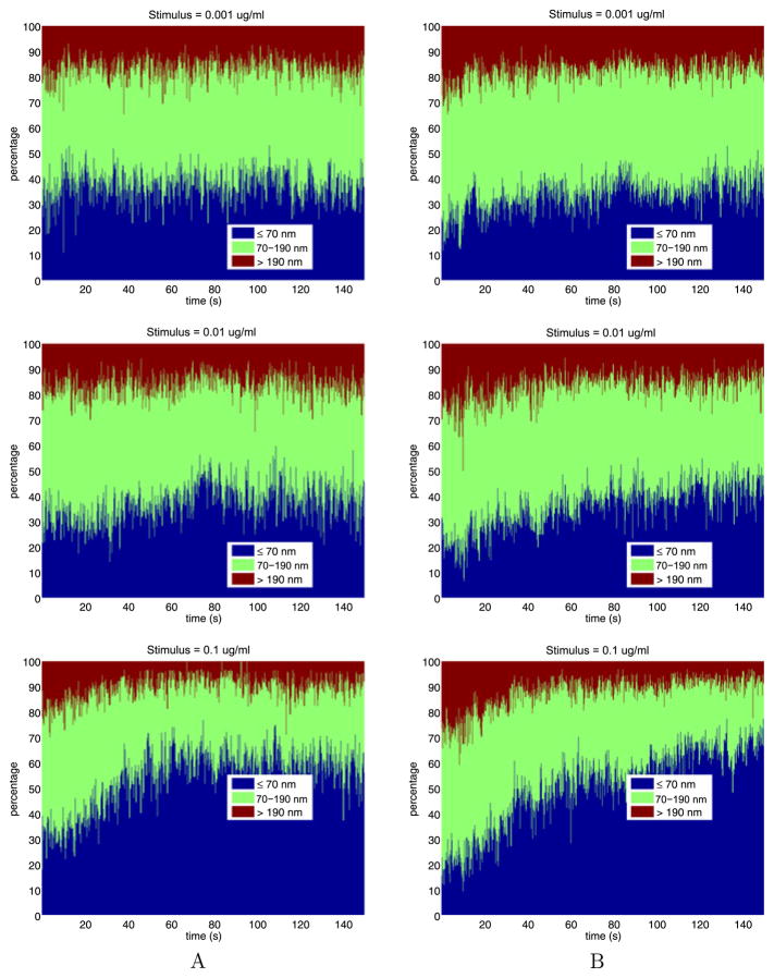
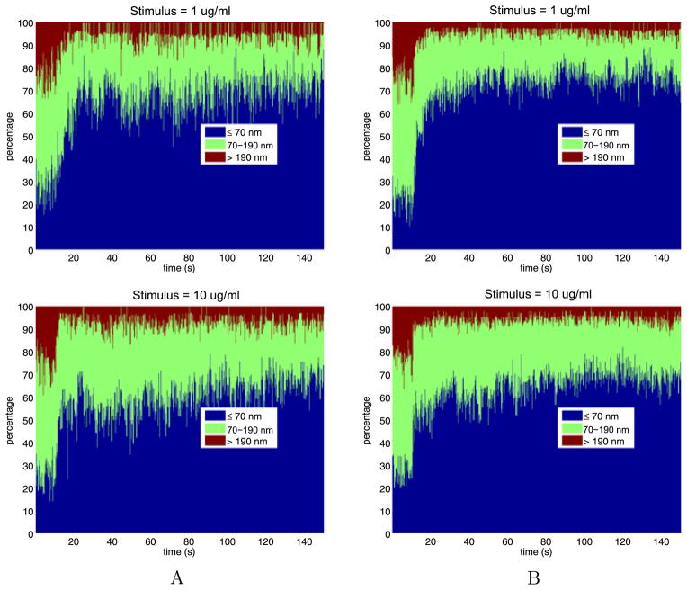
To better understand the dependence of the jump sizes on stimulus and time, we divide the jump sizes into three bins: short jumps that are smaller than 70 nm; medium jumps that are between 70 nm and 190 nm; and long jumps that are greater than 190 nm. Figure 10 shows how the percentage of jump lengths changes over time with increasing stimulus. From these figures we see that, as time increases, not much changes for weak stimuli, while for strong stimuli there is a substantial increase in the percentage of short jumps and a substantial decrease in percentage of long jumps.

Fig. 10.

The time- and stimulus-dependent percentages of the jump lengths

5.1 Analyzing the Slowing

Now we quantify the transition from diffusion in the unstimulated cells to that when the cells are stimulated. We do this by fitting the standard deviation with both a decaying exponential and a power law. The exponential fit of the jump sizes is given by a function of the form

$$S(t)=(S_l-S_r)e^{-max(0,(t-t_s))/t_m}+S_r.$$

The fit S(t) is the approximation to the standard deviation, t is the time in seconds, t_s = 10 sec (200 time steps) is the time at which the cells were stimulated, and t_m, S_l and S_r are parameters to be computed. The function S(t) is the constant S_l for 0 ≤ t ≤ t_s and then, as time increases, decays exponentially to the value S_r; see Fig. 9. To capture any scaling behavior, we used a power-law fit of the form

$$S(t)=\frac{S_l-S_r}{(1+\frac{max(0,t-t_s)}{t_s})\beta }+S_r.$$

Again, β, S_l and S_r are to be computed and S(t) is the constant S_l for 0 ≤ t ≤ t_s and has a power-law decay to S_r. The power β is dimensionless. The coefficients for these fits are given in Table 7.

Table 7.

The parameters for the exponential and power-law fits of the time-dependent standard deviation of the jump lengths for data sets A and B. Column 2 gives the number of jumps used in the fit, r is residual for the fit. The stimuli are divided into weak (W, 0.001, 0.110) and strong (S, 0.100, 1.000, 10.000)

Stimulus			Jumps	Exponential fit				Power-law fit
				Sl	Sr	tm	r	Sl	Sr	β	r
A	W	0.001	85,752	121.36	112.09	0.09	14.1	121.36	112.09	115.66	14.1
	W	0.010	96,007	121.41	107.68	40.16	14.1	123.48	102.41	0.46	14.2
	S	0.100	89,262	124.16	80.35	19.31	14.4	125.34	73.38	0.82	14.7
	S	1.000	61,889	125.51	64.93	5.08	14.8	125.98	64.41	2.62	14.9
	S	10.000	91,032	133.15	78.15	1.14	13.8	133.18	78.14	9.47	13.8
B	W	0.001	122,435	131.04	114.90	26.43	12.7	132.81	110.65	0.65	12.6
	W	0.010	106,451	134.93	107.19	32.48	13.4	136.31	83.61	0.31	13.4
	S	0.100	119,108	142.22	80.68	30.09	12.4	144.48	31.50	0.33	12.3
	S	1.000	122,970	138.50	62.66	4.81	11.4	139.00	61.79	2.58	11.3
	S	10.000	139,102	130.91	75.46	2.52	11.4	130.18	74.88	3.43	11.3

For the weak stimuli, the fitting program produced erratic results, that is, if we changed the initial guesses or the parameters in the fitting algorithm, the results for the parameters would change, but the quality of the fits remained the same. This behavior is caused by the large noise in the data and the small changes in the standard deviations. As a consequence, the fits for the weak stimuli are not reliable. In particular, in Fig. 9, the plot of data set A for stimulus 0.001 has an unreasonably rapid change for small time, consequently the corresponding value for β in Table 7 is unreasonably large. On the other hand, for the strong stimuli, the fits are excellent. In all cases, both the exponential and power-law fits are very close to each other. The exponential fits provide a mean lifetime that quantifies how much faster the transition between fast and slow motion occurs as the stimulus increases. For the strong stimuli cases, the exponential fits agree with those found in Andrews et al. (2008).

For both fits, the values of S_l are estimates of the standard deviation of the jumps in unstimulated cells, which are close to the values given in Table 3, but are based on much smaller data sets given by 0 ≤ t ≤ t_s and thus have more noise. For the strong stimuli, S_r gives an estimate of the standard deviation of the jumps in the tail which are from 45 % to 60 % of the standard deviation compared to when the cells are unstimulated. It is interesting that for the strong stimuli, S_r decreases for the stimuli going from 0.100 to 1.000, but then increases slightly for stimulus 10.000.

In the exponential fit, the coefficient t_m has units of seconds and is called the mean lifetime (the half-life is $\sqrt{2}{t}_m$) and gives the time t − t_s in seconds where S(t) = S(t_s)/e. The mean lifetime t_m is erratic for weak stimuli. For the strong stimuli, the mean lifetimes range from 30 to 1 s. In the literature, after a small multiple of these times, the QDs are said to be immobilized. However, as the standard deviation never drops much below one half of the standard deviation before stimulation, complete immobilization is never achieved. In the power-law fits, a value of β ≤ 3 indicates a very slow decay, which happens in four cases for the strong stimuli. Also, for increasing strong stimulus, the mean lifetime steadily decreases and the exponent β in the power-law fit steadily increases.

5.2 Analyzing the Tails

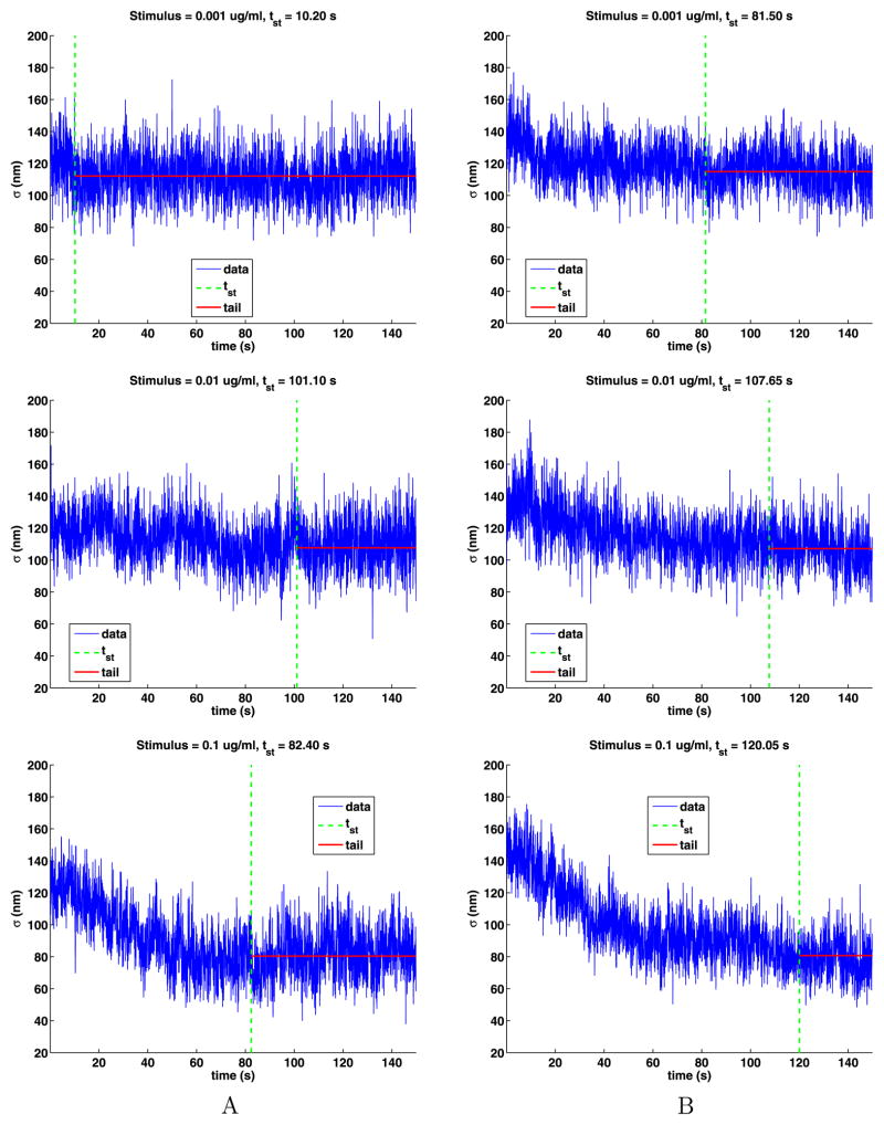
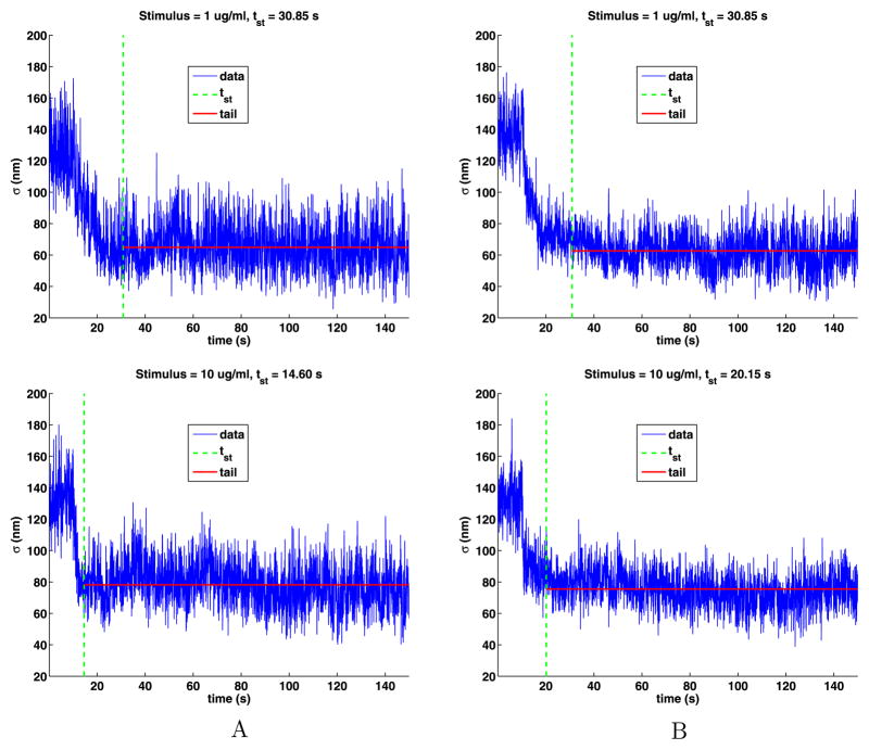
Using the exponential fit, we estimate the time t_st at which the motion becomes stationary by computing the smallest time t_st for which S(t_st) − S_r ≤ 1 nm. The exponential and power-law fits give essentially the same value. The tail of the time series is defined as the data for times t such that t_st ≤ t ≤ 150 s and are illustrated in Fig. 11. Table 8 gives the values of t_st and the number of jumps in the tails, which is quite large. For weak stimuli, the results for t_st are erratic, but for strong stimuli the times decrease with increasing stimuli. The times t_st for strong stimuli are from 4 to 13 times longer than the mean lifetimes given in Table 7.

Fig. 11.

The time-dependent standard deviations of the tails with their stationary times marked by a vertical dashed line and the mean value of s for the tails given by a horizontal solid line

Table 8.

The stimulus, the time at which the time series becomes stationary (t_st), and the number of jumps in the tail. The weak (W) and strong (S) stimuli are separated by an empty line

Stimulus		A		B
		tst	Jumps	tst	Jumps
W	0.001	10.20	80,522	81.50	56,017
W	0.010	101.10	27,475	107.65	31,341
S	0.100	82.40	34,810	120.05	22,822
S	1.000	30.85	47,662	30.85	94,559
S	10.000	14.60	81,890	20.15	121,932

In Table 9, we present the standard deviation σ_r of the jumps computed using (25) where σ_x and σ_y are the standard deviation of the jump components given in Table 14. The values of σ_r before stimulus are close to those for the unstimulated data considering that they are based on significantly smaller data sets. With increasing stimulus, the values of σ_r in the tails decrease dramatically, but we do see a modest increase for the stimulus 10 μg/ml. For ease of comparison with the literature, the diffusion coefficients given by (15), using units of nm²/μs = μm²/s, are included in the table. Note that, for example, in data set A for stimulus 1.000, the standard deviation decreases by a factor of 2 after stimulation, but the diffusion coefficient is reduced by a factor of 4. Thus, using the diffusion coefficient to measure slowdown exaggerates the slowing of the motion compared to using the standard deviation. Indeed, the units of the standard deviation and the diffusion coefficient imply this.

Table 9.

For the stimulated cell data, the standard deviation σ_r of the jump lengths and the diffusion coefficient D, both before stimulation and in the tails for data sets A and B. The weak (W) and strong (S) stimuli are separated by an empty line. For comparison, values for unstimulated (U) data are included

Stimulus			Before stimulus			Tail
			Jumps	σr	D	Jumps	σr	D
A	U	0.000	405,600	138.00	0.0982	351,700	138.00	0.0982
	W	0.001	5,182	121.36	0.0736	80,522	112.09	0.0628
	W	0.010	6,366	118.67	0.0704	27,475	109.15	0.0596
	S	0.100	7,540	123.81	0.0766	34,810	81.79	0.0334
	S	1.000	4,376	124.99	0.0781	47,662	65.20	0.0213
	S	10.000	6,165	132.85	0.0882	81,890	78.21	0.0306
B	U	0.000	351,700	139.50	0.0973	351,700	139.50	0.0973
	W	0.001	6,896	136.82	0.0936	56,017	114.70	0.0658
	W	0.010	5,948	137.60	0.0947	31,341	107.61	0.0579
	S	0.100	8,082	144.31	0.1041	22,822	78.62	0.0309
	S	1.000	7,839	139.24	0.0969	94,559	62.39	0.0195
	S	10.000	8,423	132.59	0.0879	121,932	75.28	0.0283

Table 14.

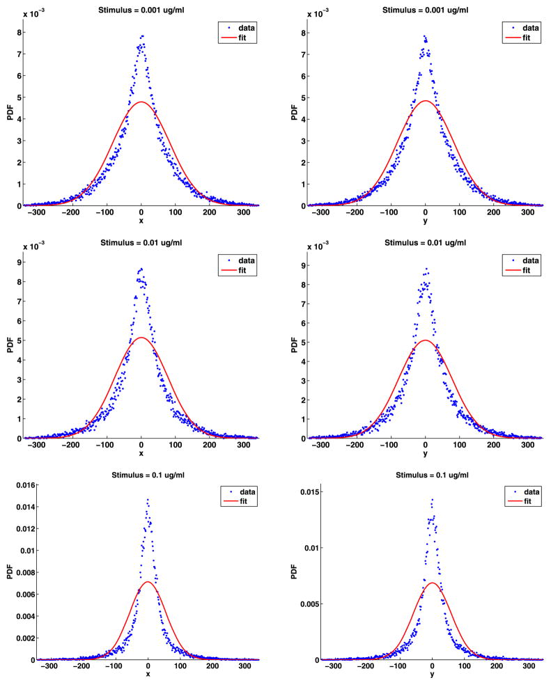
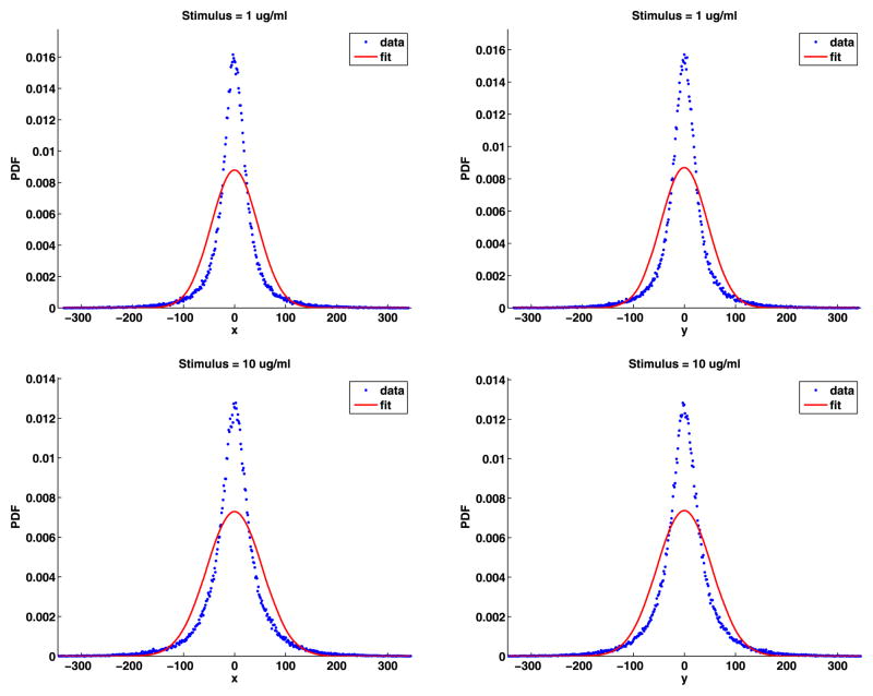
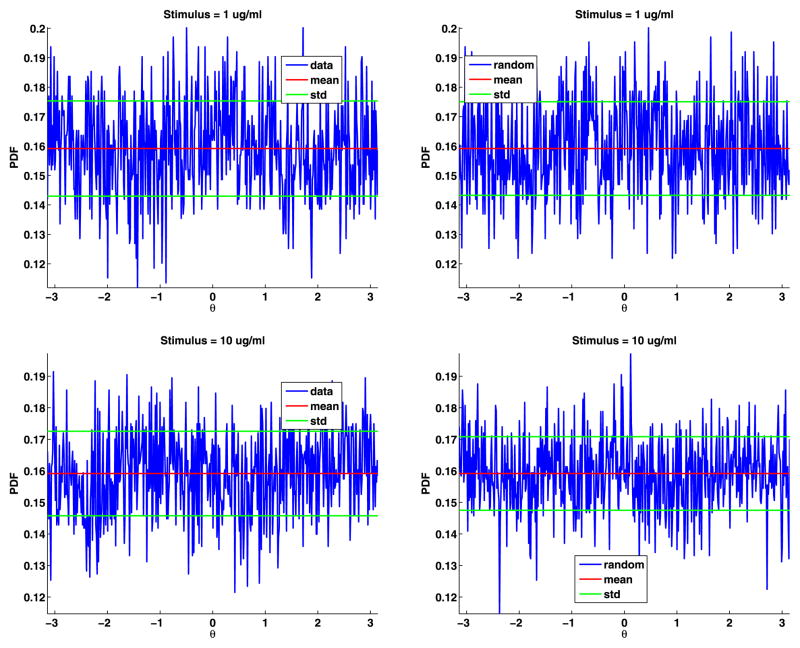
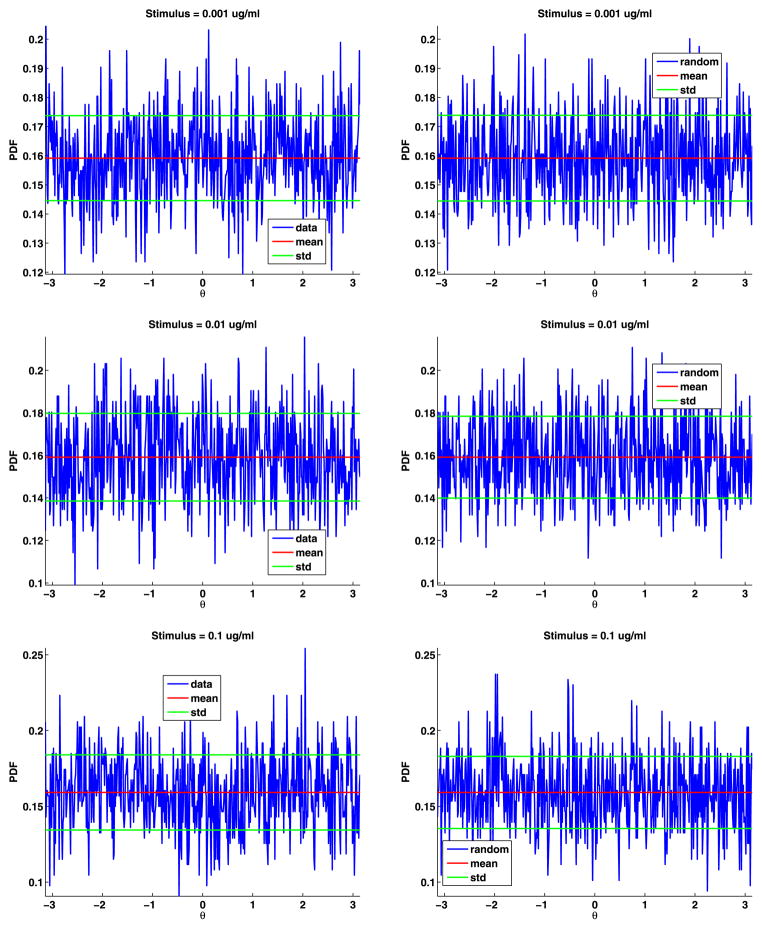
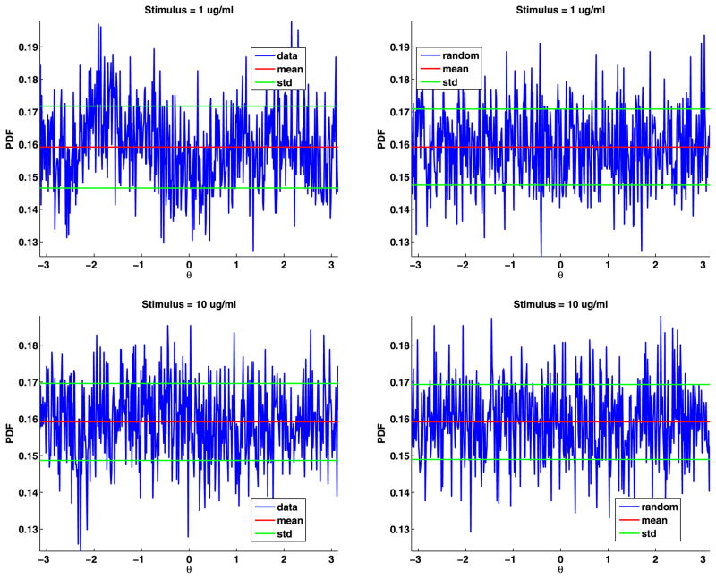
Tail data sets A and B: stimulus s, mean, standard deviation and mean zero test for the x and y jump components of the PDFs shown in Figs. 20 and 21

s		Jumps	x			y
			μx	σx	μx/σx	μy	σy	μy/σy
A	0.001	80,522	−0.05	80.9	−0.0006	−0.09	81.9	−0.0011
	0.010	27,475	0.82	78.8	0.0104	0.00	80.0	0.0000
	0.100	34,810	0.05	59.4	0.0008	0.09	60.4	0.0015
	1.000	47,662	0.31	49.5	0.0062	0.03	47.9	0.0006
	10.000	81,890	−0.20	56.9	−0.0036	0.05	57.6	0.0009
B	0.001	56,017	0.04	83.4	0.0004	0.44	82.2	0.0054
	0.010	31,341	0.33	77.6	0.0042	−0.16	78.2	−0.0020
	0.100	22,822	−0.97	56.0	−0.0173	0.08	58.1	0.0014
	1.000	94,559	−0.08	45.4	−0.0018	−0.40	45.9	−0.0087
	10.000	121,932	0.01	54.7	0.0001	−0.21	54.1	−0.0038

For the tail data, Table 10 gives the percentages, averaged over time, of the jump sizes in the bins shown in Fig. 10. With the exception of stimulus 10.000, with increasing stimulus, the percentage of short jumps increases from about 30 % to about 80 %, the percentage of medium jumps decreases from about 50 % to about 17 %, while the percentage of long jumps decreases from about 17 % to about 3 %. These trends reverse slightly for stimulus 10.000.

Table 10.

For the tail data, the percentage of jump lengths (nm) for data sets A and B

Stimulus	A			B
	≤70	70–190	>190	≤70	70–190	>190
0.000	32.89	49.68	17.44	30.80	51.37	17.83
0.001	46.56	43.27	10.17	44.97	44.55	10.48
0.010	48.94	41.34	9.72	50.94	39.83	9.23
0.100	68.97	26.44	4.59	72.55	23.31	4.14
1.000	77.48	20.40	2.12	81.11	17.02	1.87
10.000	69.30	27.21	3.49	72.17	24.78	3.06

From Fig. 11 (and from Figs. 9 and 10), it appears that the tail data is ergodic and stationary, so that we can apply the techniques used to analyze the data from unstimulated cells to the tail data from stimulated cells. Many details of the analysis are given in Appendix D as they are very similar to what was done for the unstimulated data. In particular, the autocorrelation coefficients in the tails (see Table 15) are sufficiently small to justify assuming the jumps in the tails are independent. As before, we will focus on the jump lengths. For easy comparison, we include information about the unstimulated cells in some tables.

Table 15.

The autocorrelation coefficients, C_k (k = 0, …, 5), for the tails. Recall that C₀ = 1.0 because the coefficients are normalized by the square of the standard deviation

s		tst	C1	C2	C3	C4	C5
A	0.000	0.00	0.085	−0.048	−0.024	−0.016	−0.008
	0.001	10.20	0.038	−0.056	−0.025	−0.019	−0.016
	0.010	101.10	0.061	−0.058	−0.035	−0.021	−0.018
	0.100	82.40	−0.017	−0.044	−0.014	−0.017	−0.003
	1.000	30.85	−0.090	−0.043	−0.025	−0.014	−0.004
	10.000	14.60	−0.021	−0.045	−0.023	−0.014	−0.008
B	0.000	0.00	0.077	−0.050	−0.026	−0.015	−0.010
	0.001	81.50	0.057	−0.048	−0.027	−0.016	−0.011
	0.010	107.65	0.023	−0.066	−0.038	−0.012	−0.004
	0.100	120.05	0.010	−0.044	−0.011	−0.018	−0.012
	1.000	30.85	−0.064	−0.033	−0.020	−0.009	−0.007
	10.000	20.15	−0.040	−0.048	−0.026	−0.012	−0.007

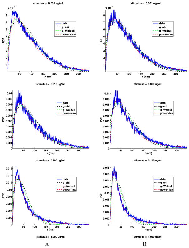
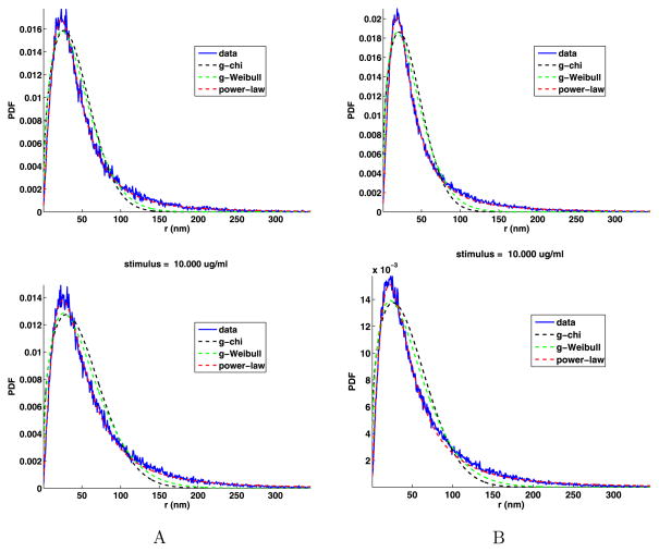
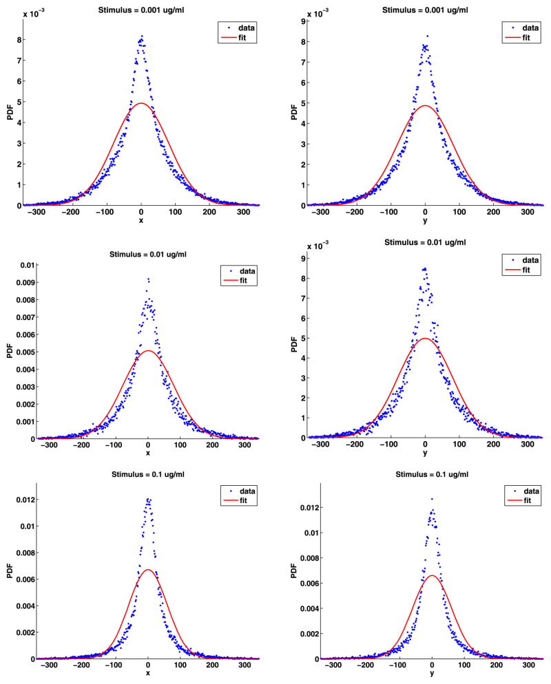
The analyses of the jump angles and components are given in Appendix D and give essentially the same results as for the jumps from unstimulated cells, that is, the jump components are not normally distributed, but the jump angles are uniformly distributed. As before, the PDFs of the jump lengths cannot have a simple chi or simple Weibull distribution, so we fit the distribution of the jump lengths with the general chi (19), general Weibull (20) and power-law (21) distributions. These fits are shown in Fig. 12 and the fit parameters are given in Table 11. This figure and the mean square errors confirm that, as before, the power-law fit is the best. The shape parameters d, k, and α are the most important. There is no apparent trend in the values of these parameters as a function of the stimulus. However, the values of d are smaller than the values of k, and the values of k are smaller than the values of α. If we estimate the fractal dimension using the chi distribution, the d is usually between about 5/4 and 4/3.

Fig. 12.

Tail jump lengths PDFs with the general chi, general Weibull and power-law fits

Table 11.

General chi, general Weibull and power-law fit parameters to the PDF of the jump lengths of the tail, and their relative mean square errors (e), for data sets A and B. The last column is the power-law exponent given by (24). The weak (W) and strong (S) stimuli are separated by an empty line

Stimulus			General chi			General Weibull			Power law
			d	s	e	k	s	e	α	β	s	e	γ
A	W	0.001	1.20	96.1	0.029	1.35	98.9	0.015	1.49	3.60	167.3	0.011	4.88
	W	0.010	1.21	89.8	0.041	1.36	93.2	0.024	1.58	2.73	111.8	0.017	3.73
	S	0.100	1.28	51.4	0.060	1.41	56.3	0.038	1.96	1.76	36.3	0.007	2.48
	S	1.000	1.44	40.5	0.035	1.55	47.6	0.023	2.02	2.04	39.8	0.003	3.10
	S	10.000	1.34	51.4	0.039	1.46	57.7	0.023	1.89	2.04	47.3	0.003	2.97
B	W	0.001	1.25	95.6	0.025	1.40	101.5	0.013	1.53	4.07	193.0	0.010	5.69
	W	0.010	1.22	85.3	0.046	1.36	89.1	0.027	1.66	2.33	85.9	0.015	3.20
	S	0.100	1.27	45.3	0.071	1.39	49.6	0.046	2.00	1.68	29.7	0.008	2.36
	S	1.000	1.36	35.0	0.050	1.48	40.0	0.032	2.05	1.80	27.7	0.002	2.64
	S	10.000	1.30	48.1	0.045	1.42	53.0	0.026	1.88	1.94	40.0	0.003	2.77

For power laws, the exponent must satisfy γ > 1 and if the analytic distribution function is to have a finite moment of order k, then it must be the case that γ − k > 1. Thus, if γ < 3, the analytic distribution function does not have a finite second moment and consequently the distribution is termed anomalous in the sense of being super diffusive (Saxton and Jacobson 1997; Metzler and Klafter 2000; Zaslavsky 2002). In the data sets A and B, there are five cases that meet the conditions for being super diffusive. As the cell has finite size, we cannot have superdiffusion due to large jumps. But still, when γ ≤ 3, the sizes of the intermediate length jumps do scale as a power law as in anomalous diffusion. We comment more on this in Sect. 6.

5.3 Summary

For the stimulated data, we break up the time series into three parts, the motion before stimulation, a period after the stimulus is added where the motion slows, and the tail where the motion resembles that for the unstimulated cells but is slower. We classify the stimuli into weak (0.001, 0.010 μg/ml) and strong (0.100, 1.000, 10 μg/ml). The effects of the weak stimuli are small and difficult to quantify because of the noise in the data. If some parameter depending on the stimulus has a trend for s < 10 μg/ml, then this trend typically, but not always, reverses slightly for s = 10 μg/ml.

We use curve fitting to study the slowing of the diffusion and then use the techniques developed in Sect. 4 to study the motion in the tails. For the strong stimuli, the mean lifetime of the change from the motion in unstimulated cells to the stationary motion in the tails of the time series decreases rapidly with increasing stimulus. The transition between the fast and slow states is rapid, occurring in a few to tens of seconds. For the tails, we also divide the jumps into short, medium and long and see that, as time increases, the number of short jumps increases significantly while the number of long jumps decreases.

For times that are in the tails of the data, the motion slows with increasing stimulus, but has a slight increase for stimulus 10.000. The jump components in the tails are not normally distributed and the normal fits to the PDFs of the components of the jumps imply that there is a higher proportion of short jumps than in the data from unstimulated cells. As before, the jump angles are uniformly distributed. For the data from stimulated cells, especially for the stronger stimuli, the power-law fits to the jump sizes is significantly better that the general chi or general Weibull. The values of d for the chi distribution suggest that the motion of the QDs can be modeled as diffusion in a fractal space of dimension between 5/4 and 4/3.

A striking aspect of the tails for strongly stimulated cells is that their statistics do not change significantly as a function of time, suggesting that nothing that significantly affects diffusion on the membrane has happened in the last two minutes of the experiments.

6 Discussion

Our results have important implications for improving our understanding of membrane organization and dynamics. Previous high-resolution electron microscopy experiments have shown that the extent of receptor clustering increases with increasing stimulus (Andrews 2011; Wilson et al. 2002; Seagrave et al. 1991). In Espinoza et al. (2012), we used hierarchical clustering and dendrograms to improve the quantification of clustering observed using TEM methods. The new dynamic data confirm that receptor mobility decreases dramatically under conditions that support the formation of larger clusters of crosslinked receptors (Andrews et al. 2009). However, the crosslinked receptors are not all strictly immobile since long and medium sized jumps have a significant presence in the tails of the data sets. The continued presence of longer jumps could reflect the transient release of QD-IgE-FcεRI complexes within the clusters from their DNP-BSA tether or it could also be that not all receptors join a crosslinked cluster. The increase in short jumps suggest that the tethers remain somewhat flexible, enabling limited mobility even in highly crosslinked IgE-FcεRI complexes or the whole cluster could be moving in short jumps.

In Sect. 3, we showed how to apply time-series analysis to understand the motion of quantum dot-labeled proteins in the cell membrane. We emphasize analyzing the jumps in the data as this gives access to the information about the smallest spatial and time scales supported by the data. We also show how to compensate for the blinking of the quantum dot labels.

In Sect. 4, we showed that it is reasonable to model the jumps between successive movie frames as ergodic stationary IID time series. Next, we showed that the jump components are not normally distributed, but the jump angles are uniformly distributed, therefore the jump lengths cannot have a simple chi or Weibull distribution. We then fit the jump lengths distribution with general chi, general Weibull and power-law distributions. The best fit was given by the power law, but all fits were quite good. The fit by the chi distribution suggests viewing the motion of the receptors as diffusion in a fractal space of dimension d < 2. By comparing the general chi and Weibull fits to the simple chi and Weibull distributions, we see that there is an excess of jumps under 70 nm, again implying that there are significant barriers to the diffusion at scales much less than 70 nm. Importantly, the distributions of the jump lengths are smooth, implying that barriers to the diffusion exist at all scales from a few tens of nanometers up to hundreds of nanometers. This implies that the barriers to normal diffusion do not have any special size.

In Sect. 5, the motion of the receptors in stimulated cells is divided into three types: the same motion as in unstimulated cells up to the time when the stimulus is added, a slowing of the motion, and a tail of stationary motion like that in unstimulated cells, only slower. We also divide the stimuli into two categories, weak and strong. For weak stimuli, the statistics of the motion tends to be noisy. For strong stimuli, the motion slows rapidly (in a few seconds to tens of seconds) and then has a long tail of stationary motion. The stationary motion implies that nothing important happens to the diffusion for two minutes starting shortly after stimulation. Again, the chi distribution d parameter for the tails suggests that diffusion is taking place in a fractal space of dimension d < 2. For strong stimuli, many of the quantities show a trend, consistently increasing or decreasing for increasing stimuli. On the other hand, some quantities show a more complex pattern. When going from s = 0.1 to 1.0, the quantity decreases, but when going from s = 1.0 to 10.0, the quantity increases some, but does not return to the level at s = 1.0 (concave up). The other possibility is the reverse: when going from s = 0.1 to 1.0, the quantity increases, but when going from s = 1.0 to 10.0 the quantity decreases some, but does not return to the level at s = 1.0 (concave down). We do not have an explanation for these reversals.

The time-series analysis in this paper and the previous cluster analysis (Espinoza et al. 2012) of the biological data has set the stage for further exploration of tracking data that may improve the understanding of the organization of the cell membrane and its impact on the biology of the cell (Cebecauer et al. 2010). It is important that the results for the time t_st for the motion to become stationary are consistent with the cluster analysis which shows that after 1 min, a fraction of the receptors forms clusters while a significant number remain unclustered, but more of the receptors are in clusters as the stimulus increases. The model will not use normally distributed jump sizes, but rather use a power-law distribution like that discovered in this paper.

It is important to have good estimates for the errors in the positions of the QDs (Destainville and Salome 2006; Wells et al. 2010; Savin and Doyle 2007), the most important of which are the localization error in measuring the position of a stationary QD, and the time averaging of the position of the quantum dot due to the camera collecting photons for essentially the full frame, in our case 1/20 s. Additionally, the QD can be displaced vertically. For our data, the localization errors for the centers of the QD have been estimated at 50 nm in Andrews et al. (2008), Andrews (2011) for a QD similar to QD625 and a faster frame rate of 33 per second. These error estimates are based on fitting the mean squared displacement which may be confounded by the algorithm that builds paths out of segments. Also, the faster frame rate would increase the errors. This result is inconsistent with our measurements of the jump component size distributions, that is, if the errors are mean zero normally distributed with standard deviation of 50 nm, then the measured jump distribution would be the convolution of the error distribution and the true jump distribution. Such a convolution would result in a measured distribution the would be close to normal, contrary to our finding of far from normal distributions.

We have developed two new methods for estimating the errors in the positions of the quantum dots that are based only on data from two successive time frames (there is no fitting) and are of the hidden Markov type. For simulated data, these methods produce excellent results for large errors, but unexpectedly, noisy results for small errors. Further work is needed for estimating small errors, but the results for our data are consistent with the errors being smaller than 20 nm.

An important problem in interpreting our results is that the QD is attached by a flexible link to the receptor, which affects the interpretation of the jump lengths. We also need a more realistic biological interpretation of the fact that the jumps are not normally distributed. One possibility is that the diffusion is anomalous. Following the discussion in review of anomalous diffusion (Metzler and Klafter 2000), there are three possibilities: normal diffusion, superdiffusion and subdiffusion. Superdiffusion is characterized by having a large excess of big jumps, which we do not see in our data. If we did see this, the more likely explanation would be that directed motion is involved, for example, motion along actin or microtubules. A more likely alternative is that the motion is subdiffusive, that there is a large excess of long pauses in the motion. Again, we do not see this in the data. Although diffusion in fractals is a special case of subdiffusion, we see no evidence of very long delays. The remaining possibility is that the motion is regular diffusion for which the Central Limit Theorem implies that the positions of many walkers starting at the same initial position will become normally distributed after some time. Our results and a preliminary analysis of multiple jump data indicates that this is not the case. Further work is required to resolve these issues.

In summary, the mast cell membrane complexes IgE-FcεRI are in continuous random motion as can be seen from the data from unstimulated cells. The movement is restricted, though, by a continuous distribution of barriers which reduces the fractal dimension of the diffusion to a value d < 2. Adding the antigen causes the complexes to slow down significantly (by about half for the strong stimuli from the point of view of jump length standard deviations or equivalently, by about one fourth from the point of view of diffusion coefficients). In addition, the slowdown occurs rapidly, on the order of 5–20 seconds for the strongest stimuli. We believe that this rapid slowdown is primarily due to protein aggregation as other possible causes such as the binding of adaptor molecules and/or recruitment into endocytic compartments (clathrin coated pits) which could significantly alter receptor mobility are downstream events that would occur at later times than those represented in the tracking data. Finally, even though many of the complexes in the tails of the tracking data are in dimers or clusters, the complexes still undergo significant motion, but now the barriers to movement restrict the motion further, lowering the fractal dimension even more.

Appendix A: Examples of Long Paths and Segments

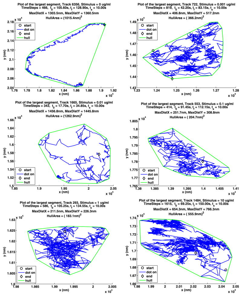
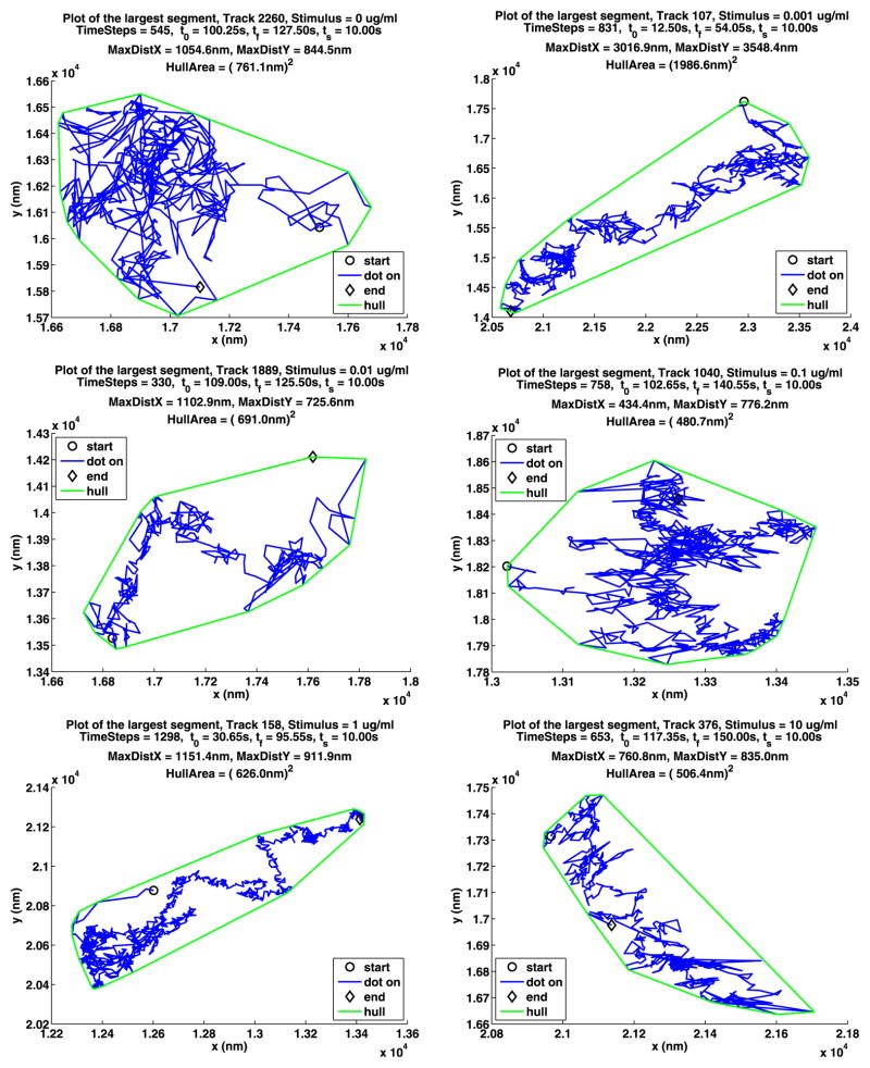
In this appendix, we extend the information about the longest paths introduced in Sect. 2. We first show the longest paths, then the longest segments, and then replot these tracks and color code the jumps by length. The main point is to show how highly variable the paths are.

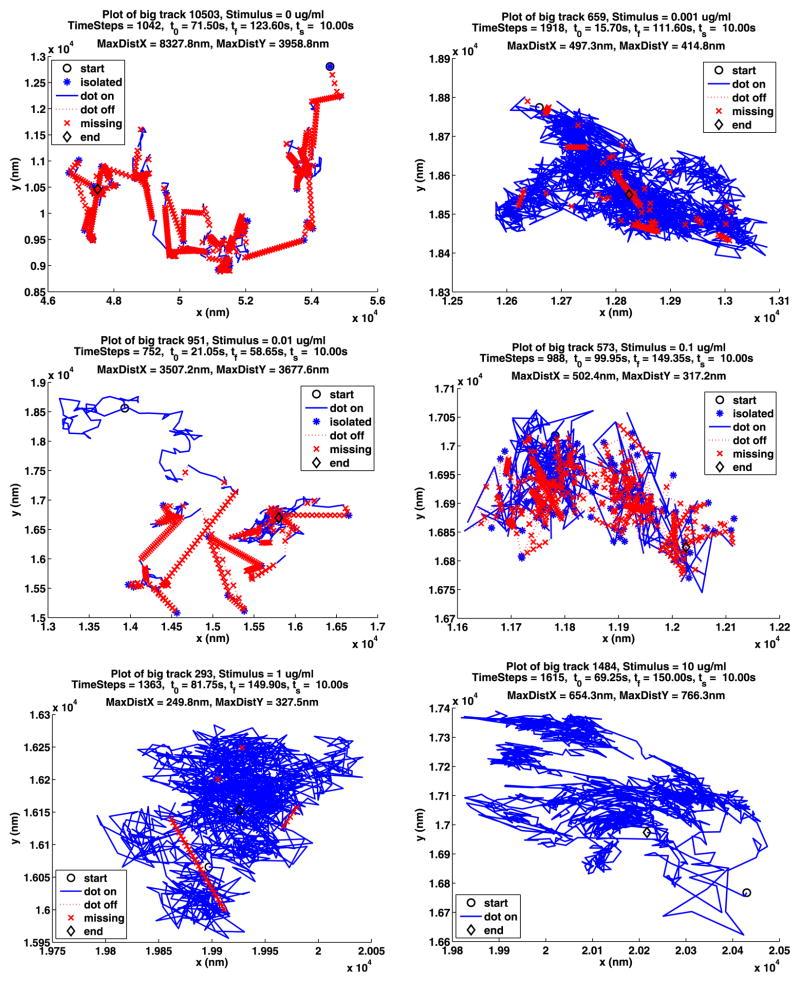
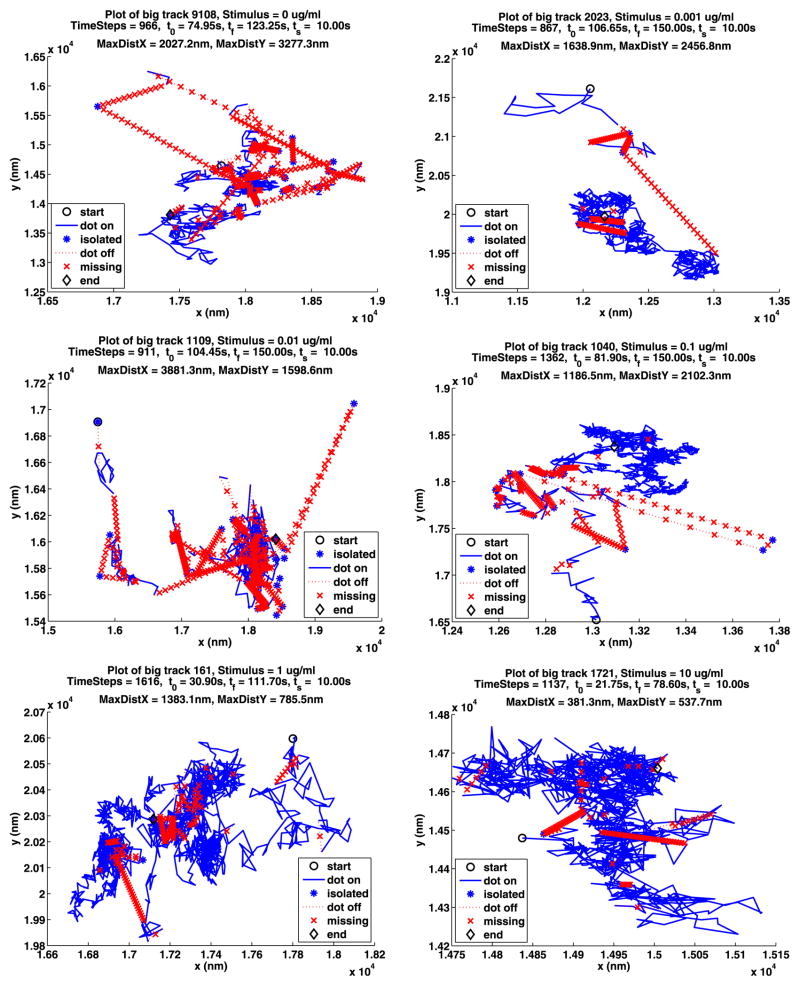
In Table 12, we summarize some information about longest paths. The parameters MDX (MaxDistX) and MDY (MaxDistY) give the size in nm of the smallest rectangle that contains the path. Figures 13 and 14 show the longest path for each stimulus for the two data sets. The plot notation is the same as that used in Fig. 2. Recall that a path is made up of segments where the QD is on, separated by segments where the QD is off, and consequently these figures also illustrate the blinking of the QDs. Note that the QDs can be on or off for a long time.

Table 12.

Paths, identified by the stimulus added and track number, with the largest number of time steps (nts) for the two data sets, A and B. MDX (MaxDistX) and MDY (MaxDistY) are the lengths of the sides of the smallest rectangle containing the path

Stimulus	A				B
	Track	Nts	MDX	MDY	Track	Nts	MDX	MDY
0.000	10503	1042	8328	3959	9108	966	2027	3277
0.001	659	1918	497	415	2023	867	1639	2457
0.010	951	752	3507	3678	1109	911	3881	1599
0.100	573	988	502	317	1040	1362	1187	2102
1.000	293	1363	250	328	161	1616	1383	786
10.000	1484	1615	654	766	1721	1137	381	538

Fig. 13.

Data set A: tracks with the longest paths

Fig. 14.

Data set B: tracks with the longest paths

Figures 15 and 16 show longest segment for each stimulus. Recall that the QD is on for all of the points in a segment. Each segment is enclosed by its convex hull. The area of the convex hull is written in the form R², so R is the length of the side of a square with the same area.

Fig. 15.

The longest segments for data set A

Fig. 16.

The longest segments for data set B

In Figs. 17 and 18, we use different colors for the jump sizes L: blue for 0 ≤ L ≤ 70 nm, green for 70 < L ≤ 190 nm, and red for 190 < L ≤ 346 nm. From these figures, we can see how the number of jumps less than or equal to 70 nm (blue) increases as the stimulus increases, while there are very few of the longest jumps.

Fig. 17.

The longest segments and their different jump lengths for data set A

Fig. 18.

The longest segments and their different jump lengths for data set B

Appendix B: QD Blinking Times

It is important for our analysis to understand that, due to the blinking of the QDs, very few QDs are on at any given time step. The minimum, mean, and maximum of the dots that are on at any given time are given in Table 2. Because only a few QDs are on at a given time, statistics that are a function of time will be noisy. The lengths of the QD on times are strongly dependent on the algorithm that connects dots at successive time steps, while the off times are strongly dependent on the algorithm that connects runs of on times. It is known that the on and off times of the QDs satisfy a power law with a negative exponent of approximately 3/2 (Bachir 2006), so we fit the function that gives the number of on and off times of a given length by

$$\text{on}(i)=q_1{i}^{-p_1},\text{off}(i)=q_2{i}^{-p_2}.$$

It is not expected that the on times will be affected by the stimulus, but it is possible that the off times are affected as the motion is slower and thus it may be easier to estimate where a dot that has turned off will turn on. The power p₁ for the on times is approximately 4/3 for all conditions (see Table 13). This is somewhat slower than that given in (Bachir 2006). The power p₂ for off times is approximately 1 (see Table 13). Note that it is common to divide the on or off times by the total number of times so that one obtains a probability distribution. However, for this to work, the power must be greater than 1. In our case, the number of off times is bounded by the number of time steps in a track, so with a power less than 1, we still get a probability distribution.

Table 13.

The power-law decay for the on and off times of the QDs for data sets A and B

Stimulus	A		B
	On	Off	On	Off
	p1	p2	p1	p2
0.000	1.27	1.02	1.26	0.89
0.001	1.33	1.00	1.26	0.92
0.010	1.29	0.96	1.29	0.94
0.100	1.32	0.95	1.28	0.92
1.000	1.39	0.98	1.24	0.91
10.000	1.36	0.94	1.31	0.93

In the off times data, the off times are zero after 32 time steps. This is caused by the path construction algorithm, which connects segments of on times, having a limit of 32 off times in between the on times. Because of this, the power-law fit was made using the first 32 data points.

Appendix C: Problem with Large Jumps

During our analysis, we noticed a problem with the large jump lengths. We used the material in Sect. 3.6 with 500 bins to estimate the PDF of the jump lengths and display these in Fig. 19. We see that the data analysis algorithms that construct the paths introduce a dramatic reduction in the number of jumps at 346 nm. Therefore, in our analysis we discarded all jumps bigger than 346 nm. This is a very small percentage of the total data: 2,069 jumps or less than 0.5 % of the data for data set A; and 1,668 jumps or less than 0.5 % of the data for data set B.

Fig. 19.

PDFs of all the jump lengths for the data sets A and B

Appendix D: Analysis Details for the Tail Data

In this appendix, we provide some of the details about the tail data that was not discussed in Sect. 5. We begin by showing that the tail jump components can be modeled as mean zero. We next compute the autocorrelations coefficients to support modeling the jumps as independent. Thus, as with the unstimulated data, we will model the tail jump data as IID and mean zero and estimate the statistics for the data in the tails using the formulas in Sect. 3.4. Next, we give more details concerning the PDFs of the tail jump components and the jump angles.

In Table 14, we expand on information about the statistics of the tail jump components first presented in Table 9. Note that the dimensionless means μ/σ are small, which justifies modeling the tail data as mean zero. Also, note that the standard deviations σ_x and σ_y decrease with increasing stimulus except for the slight increase at stimulus 10 μg/ml for both data sets.

Table 15 gives the first six autocorrelation coefficients for the tail data. We include the data for the unstimulated case for comparison. The second column is the stimulus s. The third column is the time in seconds when the tail data starts. The remaining columns are the autocorrelation coefficients. C₀ = 1 because the coefficients are normalized by the square of the standard deviation (variance) and thus are dimensionless. For both the A and B datasets, C₁ goes from positive to negative as the stimulus increases. For each k > 1 the coefficients are essentially independent of the stimulus with the exception of one value in data set B with s = 1.000 and C₄ = −0.009. With three exceptions, the coefficients slowly decrease in size with increasing k ≥ 2. The behavior of C₁ is quite different from the coefficients with k ≥ 2.

In Figs. 20 and 21, we display the PDFs of the jump components in the tail data along with their fits by mean zero normal distributions. The PDFs of the jump components in the tails were found by dividing the interval −346 ≤ Δx, Δy ≤ 346 into 500 equal subintervals that were used to bin the components. The mean and standard deviation of the jumps were estimated using (18). The normal fit is given by a mean zero normal PDF with the same standard deviation as the data that are given in Table 14. As with the unstimulated data, the plots in these figures indicate that the PDFs are not normally distributed which is confirmed by the two-sample Kolmogorov–Smirnov test. In all cases, we observe that for approximately |x|, |y| < 50 nm, there is an excess of short jumps compared to the normal distribution and that this excess is bigger than in the unstimulated data. For approximately 50 < |x|, |y| < 190 nm, there are fewer jumps than in a normal distribution. Note that a bound B on |x| and |y| corresponds to a bound of $\sqrt{2}B$ on the jump size r, so 50 nm in the components corresponds to approximately 70 nm for the total jump lengths.

Fig. 20.

Distributions and their normal fits of the jump components in the tails of data set A

Fig. 21.

Distributions and their normal fits of the jump components in the tails of data set B

To analyze the jump angles, as before, we divide [−π, π] into 500 bins and then bin the angles and compute their PDFs, which are displayed in Figs. 22 and 23. As with the unstimulated data the mean angle is 0.1592 as is true for the uniform distribution which is equal to π/2. The two-sample Kolmogorov–Smirnov test gives H of zero under all stimuli for a confidence value of 0.0001, so we cannot reject the null hypothesis that the angles are uniformly distributed. The asymptotic p-values shown in Table 16 confirm this. This is very strong support for modeling the angles as uniformly distributed.

Fig. 22.

Data angles and generated random angles in the tails of data set A

Fig. 23.

Data angles and generated random angles in the tails of data set B

Table 16.

The p-values for the two-sample Kolmogorov–Smirnov test for the jump angles

Stimulus	A	B
0.0010	0.8110	0.0774
0.0100	0.2184	0.3198
0.1000	0.2184	0.0657
1.0000	0.1238	0.1436
10.0000	0.0909	0.8970

References

- Adamic L. Complex systems: unzipping Zipf’s law. Nature. 2011;474(7350):164–165. doi: 10.1038/474164a. [DOI] [PubMed] [Google Scholar]
- Andrews NL. PhD thesis. University of New Mexico; Albuquerque, New Mexico, USA: 2011. The role of diffusion and membrane topography in the initiation of high affinity IgE receptor signaling. [Google Scholar]
- Andrews NL, Lidke KA, Pfeiffer JR, Burns AR, Wilson BS, Oliver JM. Actin restricts FcεRI diffusion and facilitates antigen induced receptor immobilization. Nat Cell Biol. 2008;10(8):955–962. doi: 10.1038/ncb1755. [DOI] [PMC free article] [PubMed] [Google Scholar]
- Andrews NL, Pfeiffer JR, Martinez AM, Haaland DM, Davis RW, Kawakami T, Oliver JM, Wilson BS, Lidke DS. Small, mobile FcεRI aggregates are signaling competent. Immunity. 2009;31(3):469–479. doi: 10.1016/j.immuni.2009.06.026. [DOI] [PMC free article] [PubMed] [Google Scholar]
- Bachir AL. Characterization of blinking dynamics in quantum dots ensembles using image correlation spectroscopy. J Appl Phys. 2006;99(6) doi: 10.1063/1.2175470. [DOI] [Google Scholar]
- Barroso MM. Quantum dots in cell biology. J Histochem Cytochem. 2011;59(3):237–251. doi: 10.1369/0022155411398487. [DOI] [PMC free article] [PubMed] [Google Scholar]
- Baumann G, Place RF, Foldes-Papp Z. Meaningful interpretation of subdiffusive measurements in living cells (crowded environment) by fluorescence fluctuation microscopy. Curr Pharm Biotechnol. 2010;11:527–543. doi: 10.2174/138920110791591454. [DOI] [PMC free article] [PubMed] [Google Scholar]
- Cebecauer M, Spitaler M, Sergé A, Magee AI. Signalling complexes and clusters: functional advantages and methodological hurdles. J Cell Sci. 2010;123(3):309–320. doi: 10.1242/jcs.061739. [DOI] [PubMed] [Google Scholar]
- Destainville N, Salome L. Quantification and correction of systematic errors due to detector time-averaging in single-molecule tracking experiments. Biophys J. 2006;90(2):L17–L19. doi: 10.1529/biophysj.105.075176. [DOI] [PMC free article] [PubMed] [Google Scholar]
- Espinoza F, Oliver J, Wilson B, Steinberg S. Using hierarchical clustering and den-drograms to quantify the clustering of membrane proteins. Bull Math Biol. 2012;74:190–211. doi: 10.1007/s11538-011-9671-3. [DOI] [PMC free article] [PubMed] [Google Scholar]
- Jaqaman K, Loerke D, Mettlen M, Kuwata H, Grinstein S, Schmid SL, Danuser G. Robust single-particle tracking in live-cell time-lapse sequences. Nat Methods. 2008;5(8):695–702. doi: 10.1038/nmeth.1237. [DOI] [PMC free article] [PubMed] [Google Scholar]
- Nicolau DV, Jr, Hancock JF, Burrage K. Sources of anomalous diffusion on cell membranes: a Monte Carlo study. Biophys J. 2007;92:1975–1987. doi: 10.1529/biophysj.105.076869. [DOI] [PMC free article] [PubMed] [Google Scholar]
- Kalay Z, Parris PE, Kenkre VM. Effects of disorder in location and size of fence barriers on molecular motion in cell membranes. J Phys Condens Matter. 2008;20(24):245105, 8. [Google Scholar]
- Kenkre VM, Giuggioli L, Kalay Z. Molecular motion in cell membranes: analytic study of fence-hindered random walks. Phys Rev E. 2008;77:1–10. doi: 10.1103/PhysRevE.77.051907. [DOI] [PubMed] [Google Scholar]
- Kraft S, Kinet JP. New developments in FcεRI regulation, function and inhibition. Nat Rev Immunol. 2007;7:365–378. doi: 10.1038/nri2072. [DOI] [PubMed] [Google Scholar]
- Kubitscheck U. Single molecule fluorescence monitoring in eukaryotic cells: intranuclear dynamics of splicing factors. Wiley-VCH Verlag GmbH & Co; KGaA: 2009. pp. 1–17. [Google Scholar]
- Kusumi A, Nakada C, Ritchie K, Murase K, Suzuki K, Murakoshi H, Kasai RS, Kondo J, Fujiwara T. Paradigm shift of the plasma membrane concept from the two-dimensional continuum fluid to the partitioned fluid: high-speed single-molecule tracking of membrane molecules. Annu Rev Biophys Biomol Struct. 2005;34(1):351–378. doi: 10.1146/annurev.biophys.34.040204.144637. [DOI] [PubMed] [Google Scholar]
- Lidke DS, Andrews NL, Pfeiffer JR, Jones HDT, Sinclair MB, Haaland DM, Burns AR, Wilson BS, Oliver JM, Lidke KA. Exploring membrane protein dynamics by multicolor single quantum dot imaging using wide field, TIRF, and hyperspectral microscopy. Proc SPIE. 2007;6448:6448. [Google Scholar]
- Lidke DS, Wilson BS. Caught in the act: quantifying protein bahaviour in living cells. Trends Cell Biol. 2009;19:566–574. doi: 10.1016/j.tcb.2009.08.004. [DOI] [PMC free article] [PubMed] [Google Scholar]
- Lidke DS, Arndt-Jovin DJ. Imaging takes a quantum leap. Physiology. 2004;19(6):322–325. doi: 10.1152/physiol.00030.2004. [DOI] [PubMed] [Google Scholar]
- Lidke DS, Lidke KA, Rieger B, Jovin TM, Arndt-Jovin DJ. Reaching out for signals: filopodia sense EGF and respond by directed retrograde transport of activated receptors. J Cell Biol. 2005;170(4):619–626. doi: 10.1083/jcb.200503140. [DOI] [PMC free article] [PubMed] [Google Scholar]
- Lidke DS, Low-Nam ST, Cutler PJ, Lidke KA. Determining FcεRI diffusional dynamics via single quantum dot tracking. In: Rast JP, Booth JWD, editors. Methods in molecular biology: Vol. 748. Immune receptors. Clifton: Humana Press; 2011. pp. 121–132. [DOI] [PubMed] [Google Scholar]
- Lidke DS, Nagy P, Heintzmann R, Arndt-Jovin DJ, Post JN, Grecco H, Jares-Erijman EA, Jovin TM. Quantum dot ligands provide new insights into receptor-mediated signal transduction. Nat Biotechnol. 2004;22:198–203. doi: 10.1038/nbt929. [DOI] [PubMed] [Google Scholar]
- Lillemeier BF, Pfeiffer JR, Surviladze Z, Wilson BS, Davis MM. Plasma membrane-associated proteins are clustered into “islands” attached to the cytoskeleton. Proc Natl Acad Sci USA. 2006;103(50):18993. doi: 10.1073/pnas.0609009103. [DOI] [PMC free article] [PubMed] [Google Scholar]
- Lippincott-Schwartz J, Snapp E, Kenworthy A. Studying protein dynamics in living cells. Nat Rev Mol Cell Biol. 2001;2(6):444–456. doi: 10.1038/35073068. [DOI] [PubMed] [Google Scholar]
- Manley S, Gillette JM, Patterson GH, Shroff H, Hess HF, Betzig E, Lippincott-Schwartz J. High-density mapping of single-molecule trajectories with photoactivated localization microscopy. Nat Methods. 2008;5(2):155–157. doi: 10.1038/nmeth.1176. [DOI] [PubMed] [Google Scholar]
- Metzler R, Klafter J. The random walk’s guide to anomalous diffusion: a fractional dynamics approach. Phys Rep. 2000;339(1):1–77. [Google Scholar]
- Novak IL, Kraikivski P, Slepchenko BM. Diffusion in cytoplasm: effects of excluded volume due to internal membranes and cytoskeletal structures. Biophys J. 2009;97(3):758–767. doi: 10.1016/j.bpj.2009.05.036. [DOI] [PMC free article] [PubMed] [Google Scholar]
- Pike LJ. A report on the keystone symposium on lipid rafts and cell function. PubMed. 2006;47(7):1597–1598. doi: 10.1194/jlr.E600002-JLR200. [DOI] [PubMed] [Google Scholar]
- Pinaud F, Clarke S, Sittner A, Dahan M. Probing cellular events, one quantum dot at a time. Nat Methods. 2010;7(4):275–285. doi: 10.1038/nmeth.1444. [DOI] [PubMed] [Google Scholar]
- Pons T, Mattoussi H. Investigating biological processes at the single molecule level using luminescent quantum dots. Ann Biomed Eng. 2009;37:1934–1959. doi: 10.1007/s10439-009-9715-0. [DOI] [PubMed] [Google Scholar]
- Savin T, Doyle PS. Statistical and sampling issues when using multiple particle tracking. Phys Rev E. 2007;76:021501. doi: 10.1103/PhysRevE.76.021501. [DOI] [PubMed] [Google Scholar]
- Saxton MJ. Single-particle tracking: the distribution of diffusion coefficients. Biophys J. 1997;72(4):1744–1753. doi: 10.1016/S0006-3495(97)78820-9. [DOI] [PMC free article] [PubMed] [Google Scholar]
- Saxton MJ. Single-particle tracking: connecting the dots. Nat Methods. 2008;5(8):671–672. doi: 10.1038/nmeth0808-671. [DOI] [PubMed] [Google Scholar]
- Saxton MJ. Single particle tracking. In: Jue T, editor. Handbook of modern biophysics. Fundamental concepts in biophysics. Clifton: Humana Press; 2009. pp. 1–33. [DOI] [Google Scholar]
- Saxton MJ, Jacobson K. Single particle tracking: applications to membrane dynamics. Annu Rev Biophys Biomol Struct. 1997;26(1):373–399. doi: 10.1146/annurev.biophys.26.1.373. [DOI] [PubMed] [Google Scholar]
- Seagrave JC, Pfeiffer JR, Wofsy C, Oliver JM. The relationship of IgE receptor topography to secretion in RBL-2H3 mast cells. J Cell Physiol. 1991;148(1):139–151. doi: 10.1002/jcp.1041480117. [DOI] [PubMed] [Google Scholar]
- Serge A, Bertaux N, Rigneault H, Marguet D. Dynamic multiple-target tracing to probe spatiotemporal cartography of cell membranes. Nat Methods. 2008;5(8):687–694. doi: 10.1038/nmeth.1233. [DOI] [PubMed] [Google Scholar]
- Shumway RH, Stoffer DS. Time series analysis and its applications with R examples. New York: Springer; 2006. [Google Scholar]
- Smith CS, Joseph N, Rieger B, Lidke KA. Fast, single-molecule localization that achieves theoretically minimum uncertainty. Nat Methods. 2010;7:373–375. doi: 10.1038/nmeth.1449. [DOI] [PMC free article] [PubMed] [Google Scholar]
- Weigel AV, Simon B, Tamkun MM, Krapf D. Ergodic and nonergodic processes coexist in the plasma membrane as observed by single-molecule tracking. Proc Natl Acad Sci USA. 2011;108(16):6438–6443. doi: 10.1073/pnas.1016325108. [DOI] [PMC free article] [PubMed] [Google Scholar]
- Wells NP, Lessard GA, Goodwin PM, Phipps ME, Cutler PJ, Lidke DS, Wilson BS, Werner JH. Time-resolved three-dimensional molecular tracking in live cells. Nano Lett. 2010;10(11):4732–4737. doi: 10.1021/nl103247v. [DOI] [PMC free article] [PubMed] [Google Scholar]
- Wilson BS, Pfeiffer JR, Oliver JM. FcεRI signaling observed from the inside of the mast cell membrane. Mol Immunol. 2002;1144:1–10. doi: 10.1016/s0161-5890(02)00073-1. [DOI] [PubMed] [Google Scholar]
- Ying W, Huerta G, Zúñiga M, Steinberg S. Time series analysis of particle tracking data for molecular motion on the cell membrane. Bull Math Biol. 2009;71(8):1967–2024. doi: 10.1007/s11538-009-9434-6. [DOI] [PMC free article] [PubMed] [Google Scholar]
- Zaslavsky GM. Chaos, fractional kinetics, and anomalous transport. Phys Rep. 2002;371:461–580. [Google Scholar]