Semiparametric Bayesian local functional models for diffusion tensor tract statistics

Abstract

We propose a semiparametric Bayesian local functional model (BFM) for the analysis of multiple diffusion properties (e.g., fractional anisotropy) along white matter fiber bundles with a set of covariates of interest, such as age and gender. BFM accounts for heterogeneity in the shape of the fiber bundle diffusion properties among subjects, while allowing the impact of the covariates to vary across subjects. A nonparametric Bayesian LPP2 prior facilitates global and local borrowings of information among subjects, while an infinite factor model flexibly represents low-dimensional structure. Local hypothesis testing and credible bands are developed to identify fiber segments, along which multiple diffusion properties are significantly associated with covariates of interest, while controlling for multiple comparisons. Moreover, BFM naturally group subjects into more homogeneous clusters. Posterior computation proceeds via an efficient Markov chain Monte Carlo algorithm. A simulation study is performed to evaluate the finite sample performance of BFM. We apply BFM to investigate the development of white matter diffusivities along the splenium of the corpus callosum tract and the right internal capsule tract in a clinical study of neurodevelopment in new born infants.

Introduction

Diffusion tensor imaging (DTI) is a magnetic resonance imaging (MRI) technique that measures the diffusion orientation of water molecules in tissue. The mobility of water molecules is affected by the tissue properties of white matter fiber tracts, such as the density of the fibers, the average fiber diameter, and the directionality of the fibers. In turn, the information collected on the diffusion properties of water molecules provides the structural organization of the white matter fiber tracts (Kubicki et al., 2007). The water diffusion directions and magnitudes at each voxel in the brain can be described by a 3 × 3 symmetric positive matrix, called a diffusion tensor (DT) (Basser et al., 1994a, 1994b). The degree of diffusivity can be quantified by the three eigenvalue–eigenvector pairs of DT, and its related parameters, such as fractional anisotropy (FA) (Hasan and Narayana, 2003; Hasan et al., 2001; Pierpaoli and Basser, 1996; Zhu et al., 2006). A rich literature in neuroimaging has been developed to analyze white matter fiber tract maturation and integrity via a set of water diffusion parameters, such as FA and mean diffusivity (MD), used as biomarkers (Cascio et al., 2007; Moseley, 2002; Mukherjee and McKinstry, 2006; Rollins, 2007).

Three major analytic approaches for grouping analysis of DTI data have been explored including analyses based on region-of-interest (ROI), voxels, and fiber tracts (O’Donnell et al., 2009; Smith et al., 2006; Snook et al., 2007; Stieltjes et al., 2001; Xue et al., 1999). The region-of-interest (ROI) method (Bonekamp et al., 2008; Gilmore et al., 2008) suffers from difficulties in identifying meaningful ROIs, particularly the long curved structures common in fiber tracts, instability of statistical results, and the partial volume effect in relatively large ROIs (Snook et al., 2007). Voxel based analysis (Camara et al., 2007; Chen et al., 2009; Focke et al., 2008; Snook et al., 2005) suffers from issues of alignment quality and the arbitrary choice of smoothing extent (Ashburner and Friston, 2000; Jones et al., 2005; Smith et al., 2006; Van Hecke et al., 2009).

There is an extensive interest in the DTI literature in developing fiber tract based analysis of diffusion properties (Goodlett et al., 2009; Goldsmith et al., 2011; O’Donnell et al., 2009; Smith et al., 2006; Stieltjes et al., 2001; Xue et al., 1999; Yushkevich et al., 2008; Zhu et al., 2010, 2011). Early tract based analyses simply average fiber tract profiles over multiple subjects (Stieltjes et al., 2001; Xue et al., 1999). Recent tract based analyses consist of DTI atlas building and a follow-up statistical analysis (Goodlett et al., 2009; Smith et al., 2006; Zhu et al., 2010). DTI atlas building is primarily to establish DTI correspondence across all DTI datasets from different subjects and to extract a set of individual DTI tracts (or skeleton) with the same corresponding geometry but varying DT and diffusion properties. For instance, in Smith et al. (2006), they developed a voxel based analysis framework to construct local diffusion properties along the white matter skeleton, fitted pointwise linear regression models, and performed pointwise hypothesis tests on the skeleton. This method essentially ignores the functional nature of diffusion properties along the white matter skeleton, and thus suffers from low statistical power in detecting interesting features and exploring variability in functional data (Zhu et al., 2011). In Goodlett et al. (2009), they used functional principal component analysis (fPCA) coupled with the Hotelling T² statistic to compare a univariate diffusion property, such as fractional anisotropy, across two (or more) populations for a single hypothesis test per tract. Zhu et al. (2010, 2011) proposed a multivariate varying coefficient model based on fPCA for the analysis of fiber bundle multiple diffusion properties and their association with a set of covariates of interest such as age. In Greven et al. (2010), they developed a functional mixed effects model as a generalization of mixed effects models and fPCA for the analysis of longitudinal DTI fiber tract data. So far, frequentist inference is the primary approach for making statistical inferences in these statistical models for fiber tract based analysis of diffusion properties.

Bayesian nonparametric models incorporate infinitely many parameters to flexibly model uncertainty in an unknown random effects distribution P. A sparseness favoring approach can be accomplished through the intrinsic Bayesian penalty for model complexity (Jeffreys and Berger, 1992), which is aided through centering on a base Bayesian parametric model. The Dirichlet process (DP) (Ferguson, 1973, 1974) provides a routinely used nonparametric prior, allowing P to have an unknown discrete form that leads to global clustering of subjects. This global clustering in which two subjects are either in the same cluster for all their random effects or in completely distinct clusters ignores local differences among subjects, motivating local partition process (LPP) priors (Dunson, 2009) that accommodate simultaneous global and local clustering of subjects.

In this paper, we propose a new semiparametric Bayes approach to model the association between multiple fiber bundle diffusion properties and covariates of interest. A multivariate random coefficient model is developed to characterize heterogeneity in the shape of the fiber bundle diffusion properties among subjects, while allowing the impact of covariates to vary across subjects. We assume a nonparametric Bayesian LPP2 prior (Dunson, 2009) on the distribution of the random coefficients to facilitate global and local borrowings of information among subjects. We consider a sparse latent factor model to more flexibly capture the within-subject correlation structure and assume a multiplicative gamma process shrinkage prior on the factor loadings which allows introduction of infinitely many factors (Bhattacharya and Dunson, 2011). We propose Bayesian local hypothesis testing to identify fiber segments, where multiple diffusion properties are significantly associated with covariates of interest, while controlling for multiple comparisons. We propose a Bayesian credible band for the average effect of each covariate. Finally, we use the nonparametric LPP2 prior to randomly cluster subjects via global and local clustering. Posterior computation proceeds via an efficient Markov chain Monte Carlo (MCMC) algorithm using slice sampling (Kalli et al., 2011; Papaspiliopoulos, 2008).

Methods and materials

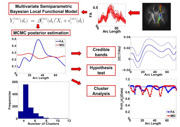
This paper focuses on developing a semiparametric Bayesian local functional model pipeline, deemed BFM, to assess the association between fiber bundle diffusion properties and a set of covariates of interest (e.g., age). Before BFM, we use DTI atlas building followed by atlas fiber tractography and fiber parametrization as described in Goodlett et al. (2009) to extract DTI fibers and establish DTI fiber correspondence across all DTI datasets from different subjects. We skip its description here for the sake of simplicity (Goodlett et al., 2009; Zhu et al., 2010). After performing the DTI atlas building step, we obtain a set of individual fiber tracts (or skeleton) with the same corresponding geometry but varying DTs and diffusion properties. Subsequently, we run the analysis pipeline BFM including a multivariate random varying coefficient model, a semiparametric Bayesian estimation method, a Bayesian approach to construct credible bands, a Bayesian local hypothesis testing procedure, and a Bayesian posterior cluster analysis procedure (Fig. 1). The computational algorithm for BFM is developed by using Matlab.

Fig. 1.

A schematic overview of BFM: a multivariate random varying coefficient model for multiple diffusion properties, an MCMC posterior estimation method for estimating the coefficient functions, a construction of Bayesian credible bands of the mean covariate effect curves, a Bayesian local hypothesis testing procedure, and a posterior cluster analysis procedure.

Multivariate random coefficient model

Assume n subjects are measured along a fiber bundle over a grid of T points for M diffusion properties (e.g. FA), denoted by {Y_i(d_t):i = 1,…,n,t = 1,…,T}, where Y_i(d_t) = ${\mathit{Y}}_i\left(d_t\right)={\left(Y_i^{\left(1\right)}\right(d_t),\dots ,Y_i^{\left(M\right)}(d_t\left)\right)}^{\prime }$ is an M × 1 vector of diffusion properties for the ith subject, d_t ∈ [0,L] is the arc length of point t relative to a fixed end point of the fiber bundle, and L is the arc length of this fiber bundle. For the ith subject, we relate the mth functional diffusion response $Y_i^{\left(m\right)}$(d_t) to a set of K covariates via a multivariate random varying coefficient model given by

$$Y_i^{\left(m\right)}\left(d_t\right)={\beta }_i^{\left(m\right)}{\left(d_t\right)}^{\prime }{\mathbf{X}}_i+{∊}_i^{\left(m\right)}\left(d_t\right),{∊}_i^{\left(m\right)}\left(d_t\right)\sim N\left(0,{\sigma }_{m,t}^2\right),$$ (1)

where X_i = ${(1,{\chi }_i^{\prime })}^{\prime }$ is the design vector for the ith subject with x_i = (x_i1,⋯,x_iK)’ being a K × 1 vector of covariates of interest, and ${\beta }_i^{\left(m\right)}\left(d_t\right)={\left({\beta }_{i,0}^{\left(m\right)}\right(d_t),\dots ,{\beta }_{i,K}^{\left(m\right)}(d_t\left)\right)}^{\prime }$ is a (K + 1) × 1 vector of random coefficients for the mth diffusion property. The measurement error ${∊}_i^{\left(m\right)}\left(d_t\right)$(d_t) is assumed to be drawn from a normal distribution with mean zero and standard deviation σ_m,t.

We model the random coefficient function ${\beta }_{i,k}^{\left(m\right)}\left(d_t\right)$(d_t) by using a linear combination of cubic B-spline basis functions b_l(d_t)s as follows:

$${\beta }_{i,k}^{\left(m\right)}\left(d_t\right)=\sum _{l=1}^p{\eta }_{\mathit{ikl}}^{\left(m\right)}{b}_l\left(d_t\right)=\mathbf{b}{\left(d_t\right)}^{\prime }{\eta }_{\mathit{ik}}^{\left(m\right)},$$ (2)

where b(d_t) = (b₁(d_t),…,b_p(d_t))’ is a p × 1 vector for B-spline basis functions and ${\eta }_{\mathit{ik}}^{\left(m\right)}={({\eta }_{\mathit{ik}1}^{\left(m\right)},\dots ,{\eta }_{\mathit{ikp}}^{\left(m\right)})}^{\prime }$’ is a p × 1 vector of random coefficients. Thus, model (1) can be written as

$$Y_i^{\left(m\right)}\left(d_t\right)={\mathit{B}}_i{\left(d_t\right)}^{\prime }{\eta }_i^{\left(m\right)}+{∊}_i^{\left(m\right)}\left(d_t\right)\text{for}m=1,\dots M,$$ (3)

where ${\eta }_i^{\left(m\right)}={({\eta }_{i0}^{{\left(m\right)}^{\prime }},\dots ,{\eta }_{\mathit{iK}}^{{\left(m\right)}^{\prime }})}^{\prime }$’ and ${\mathit{B}}_i\left(d_t\right)={\mathit{X}}_i\otimes \mathbf{b}\left(d_t\right)$ are (K + 1)p × 1 vectors. Heterogeneity in the fiber bundle diffusion properties is then controlled by the variation of ${\eta }_i^{\left(m\right)}$, which are usually treated as random effects and follow a specific parametric distribution. There is a serious concern about the sensitivity of associated inferences to the choice of the random effects distribution on the basis coefficients.

Let ${\eta }_i={({\eta }_i^{{\left(1\right)}^{\prime }},\dots ,{\eta }_i^{{\left(M\right)}^{\prime }})}^{\prime }$ be an M(K + 1)p × 1 vector, B_i = (B_i(d₁),…,B_i(d_T))’ be a T × (K + 1)p matrix, and Y_i = ${\mathit{Y}}_i={({\mathit{Y}}_i^{{\left(1\right)}^{\prime }},\dots ,{\mathit{Y}}_i^{{\left(M\right)}^{\prime }})}^{\prime }$ be an MT × 1 vector, where ${\mathit{Y}}_i^{\left(m\right)}={\left(Y_i^{\left(m\right)}\right(d_1),\dots ,Y_i^{\left(m\right)}(d_T\left)\right)}^{\prime }$ is a T × 1 vector for m = 1,…,M. The concantenated representation of model (3) is given by

$${\mathit{Y}}_i=\left({\mathit{I}}_M\otimes {\mathit{B}}_i\right){\eta }_i+{∊}_i,{∊}_i\sim {\mathit{N}}_{\mathit{MT}}(0,\Sigma ),$$ (4)

where N_MT(0,Σ) is an MT × 1 Gaussian random vector with mean zero and covariance matrix Σ = diag(${\sigma }_{1,1}^2,\dots ,{\sigma }_{M,T}^2$).

Infinite latent factor model

Given the massive dimensionality of the random effect vector η_i, it is important to favor lower dimensional representations of the dependence structure to address the curse of dimensionality. Instead of prespecifying a restrictive dependence structure, we follow the approach of using a Bayesian factor model, which relates the random effects η_i to latent factors θ_i through the following characterization

$${\eta }_i=\mathit{A}{\theta }_i,$$ (5)

where A is a (K + 1)pM × ∞ factor loading matrix and θ_i~N_∞(0,I_∞). For dimensionality reduction, one would typically restrict the dimension of the latent factor vector θ_i to be orders of magnitude less than that of η_i. However, following the motivation of Bhattacharya and Dunson (2011), we bypass the challenging issue of selecting the number of factors by incorporating infinitely many factors, while choosing a prior that favors the elements of A to be increasingly shrunk to zero as the column index increases.

We obtain the within-subject correlation structure through projecting Y_i as a linear combination of the underlying ∞-dimensional latent random vector θ_i after denoising, via

$${\mathit{Y}}_i=\left({\mathit{I}}_M\otimes {\mathit{B}}_i\right)\mathit{A}{\theta }_i+{∊}_i,{∊}_i\sim {\mathit{N}}_{\mathit{MT}}(0,\Sigma ),$$ (6)

where B_i(d_t) = X_i⊗b(d_t) and B_i = (B_i(d₁),…,B_i(d_T))^T. The common factors θ_i explain the within-subject dependence structure among the MT variables for each Y_i.

Let Y_if and ${\sigma }_f^2$ be, respectively, the fth component of Y_i and the fth diagonal element of Σ. Conditional on θ_i, Y_if1 and Y_if2 are uncorrelated for all f₁ and f₂∈{1,…,MT}. Marginalizing over the distribution of θ_i, the covariance structure Ω of the data distribution Y_i~N_MT(0,Σ) is induced as

$$\Omega =\mathrm{Var}({\mathit{Y}}_i\mid \mathit{A},\Sigma )=({\mathit{I}}_M\otimes {\mathit{B}}_i){\mathit{AA}}^T{({\mathit{I}}_M\otimes {\mathit{B}}_i)}^T+\Sigma .$$

Specifically, conditional on A and Σ, we have:

$$\begin{array}{cc}\hfill & \mathrm{Var}\left(Y_{{\mathit{if}}_1}\mid {\theta }_i,A,\Sigma \right)={\sigma }_{f_1}^2,\hfill \\ \hfill & \mathrm{Cov}\left(Y_{{\mathit{if}}_1},Y_{{\mathit{if}}_2}\mid {\theta }_i,A,\Sigma \right)=0,\hfill \\ \hfill & \mathrm{Var}\left(Y_{{\mathit{if}}_1}\mid A,\Sigma \right)={\left({\mathit{I}}_M\otimes {\mathit{B}}_i\mathit{A}\right)}_{f_1}{\left({\mathit{I}}_M\otimes {\mathit{B}}_i\mathit{A}\right)}_{f_1}^T+{\sigma }_{f_1}^2,\hfill \\ \hfill & \mathrm{Cov}\left(Y_{{\mathit{if}}_1},Y_{{\mathit{if}}_2}\mid A,\Sigma \right)={\left({\mathit{I}}_M\otimes {\mathit{B}}_i\mathit{A}\right)}_{f_1}{\left({\mathit{I}}_M\otimes {\mathit{B}}_i\mathit{A}\right)}_{f_2}^T,\hfill \end{array}$$

where (I_M⊗B_iA)_f1 is the f₁th row of (I_M⊗B_iA).

A constraint is usually specified on A to define a unique model free from identification problems, since Ω is invariant under the transformations A*=AP for any semi-orthogonal matrix P (PP^T=I). The traditional full rank lower triangular constraint for identifiability implicitly specifies order dependence among the responses (Geweke and Zhou, 1996). The choice of ordering of the response variables is a modeling decision (Carvalho et al., 2008). From the Bayesian perspective, we do not require identifiability of the loading elements in A for a wide class of applications such as covariance matrix estimation. In our case, we specify the multiplicative gamma process shrinkage prior, which will be given in Eq. (7), on a parameter expanded loading matrix with redundant parameters. The induced prior on the covariance matrix is invariant to ordering of the data. This shrinkage prior adaptively selects a truncation of the infinite loadings to one having finite columns, which facilitates the posterior computation and provides an accurate approximation to the infinite factor model.

Although FRATS (Zhu et al., 2010) and FADTTS (Zhu et al., 2011) have been proposed to analyze the DTI fiber bundle datasets of multiple diffusion measures with a set of covariates such as gender and gestational age, they assume identical effects of the covariates on the diffusion properties for all subjects. Our BFM developed here relaxes the assumption to allow the subject specific functional covariate effects on the multiple diffusion outcome functions. In addition, FRATS and FADTTS assume a covariate-free correlation structure among the multiple diffusion properties. We introduce the random factors underlying the subject specific covariate effects to allow the correlation structure among the multiple diffusion measures to vary with the levels of the covariates along the fiber tracts. Moreover, we specify an LPP2 prior on the distributions of the subject specific random factors to produce a global and local clustering structure of the multiple diffusion trajectories across the subjects.

Priors

We choose independent priors for A, θ_i, and Σ and develop an efficient Markov chain Monte Carlo (MCMC) algorithm given in Appendix A for posterior computation. To remove the redundant factors, we place the multiplicative gamma process shrinkage prior (Bhattacharya and Dunson, 2011) on the factor loading matrix A to increasingly shrink the factor loadings toward zero with the column index. This specification avoids the traditional drawback of order dependence from the lower triangular constraint for identifiability. We use inverse gamma priors on the diagonal elements of Σ. To allow a flexible latent clustering structure among subjects, we specify an LPP2 prior (Dunson, 2009) on the distribution P of θ_i. Let Ga(a,b) be a gamma distribution with scale a and shape b. Specifically, these priors are given as follows:

$$\begin{array}{cc}\hfill & \mathit{A}=\left\{A_{\mathsf{g}h}\right\},\mathsf{g}=1,\dots ,(K+1)\mathit{pM};h=1,{\dots }^{\infty },\hfill \\ \hfill & A_{\mathsf{g}h}\mid {\varphi }_{\mathsf{g}h},{\tau }_h\sim N\left(0,{\varphi }_{\mathsf{g}h}^{-1}{\tau }_h^{-1}\right),{\varphi }_{\mathsf{g}h}\sim \mathrm{Ga}(v∕2,v∕2),{\tau }_h=\prod _{l=1}^h{\delta }_l,\hfill \\ \hfill & {\delta }_1\sim \mathrm{Ga}(a_1,1),{\delta }_1\sim \mathrm{Ga}(a_2,1),l\ge 2,\hfill \\ \hfill & \zeta \sim \mathrm{Ga}(0.5,0.5),{\sigma }_f^{-2}\sim \mathrm{Ga}\left(a_{\sigma ,b_{\sigma }}\right),f=1,\dots ,\mathit{MT},\hfill \\ \hfill & {\theta }_i\sim P,P\sim \mathrm{LLP}2(\alpha ,\gamma ,P_0),P_0:{\theta }_i\sim N_{\infty }(0,\zeta {\mathit{I}}_{\infty }),\hfill \end{array}$$ (7)

where δ_l, l = 1,…,∞, are independent, τ_h is a global shrinkage parameter for the hth column, and ϕ_ghs are local shrinkage parameters for the elements in the hth column. When a₂>1, the τ_hs increase stochastically as the column index h increases, which means more shrinkage favored over the columns of higher indices. The loading component specific prior precision ${\varphi }_{\mathit{gh}}^{-1}{\tau }_h^{-1}$ allows shrinking the coefficients of the B-spline basis functions. The LPP2 prior assumption specifies an ∞-dimensional central probability measure P₀ as a prior guess, a precision parameter α expressing confidence in the prior guess, and a hyperparameter γ determining the overall allocation weight on the local family.

LPP2 prior

In modeling the multiple trajectories of diffusion measures over subjects, we are interested in identifying the latent cluster structure of Y_is among subjects, which can be induced by specifying a nonparametric prior on the unknown distribution of the random factors θ_i. Dirichlet process prior (Ferguson, 1973, 1974) is the routine approach to induce a sparse representation of subjects. However, it has the drawback of global clustering, in which two subjects are allocated to either an identical cluster or two different clusters. In DTI imaging data analysis, it is common that two subjects have similar diffusion trajectories over the major region of fiber bundles while having local deviations. Under the Dirichlet process, either such subjects are inappropriately clustered together, obscuring local differences, or allocated to separate clusters causing unnecessary computational burden. We used the LPP2 prior (Dunson, 2009) to model the unknown random effects distributions to facilitate both global and local clustering of random effects. It relaxes the global clustering assumption of the widely-used Dirichlet process prior, while accomplishing sparseness for substantial gains in computational efficiency.

After truncating the loadings matrix A to h^* ⪡ (K + 1)pM columns, we assume the resulting h^*-dimensional random effects θ_i = (θ_i1,…,θ_ih^*)^T ~ P with P unknown, i = 1,…,n. The LPP2 prior models P as a hybrid mixture distribution:

$$P=\sum _{z_1=0}^1\sum _{{\psi }_1=(1-z_1,1)}^{(1-z_1,\infty )}\cdots \sum _{z_h^{\ast }=0}^1\sum _{{\psi }_{h^{\ast }}=(1-z_h^{\ast },1)}^{(1-z_{h^{\ast }},\infty )}{\pi }_{{\psi }_1},\dots ,{\psi }_{h^{\ast }}{\delta }_{{ϴ}_{\psi }},$$ (8)

where δ_χ denotes a degenerate distribution with all its mass at χ, π_{ψ1,…,ψh^*} is the probability of θ_i = Θ_ψ having the property that π_{ψ1,…,ψh^*}≥0 and

$$\sum _{z_1=0}^1\sum _{{\psi }_1=(1-z_1,1)}^{(1-z_1,\infty )}\cdots \sum _{z_{h^{\ast }}=0}^1\sum _{{\psi }_{h^{\ast }}=(1-z_{h^{\ast }},1)}^{(1-z_{h^{\ast }},\infty )}{\pi }_{{\psi }_1},\dots ,{\psi }_{h^{\ast }}=1.$$

The indicator z_j~Ber(ν_j), j=1,…,h^*, denotes the allocation to global clustering or local clustering, taking the value of 1 for global clustering and 0 for local clustering. The hybrid atom ${ϴ}_{\psi }={\left({ϴ}_{{\psi }_{1,}1,\dots ,}{ϴ}_{{\psi }_h^{\ast },h^{\ast }}\right)}^T$ is obtained by setting the jth element of Θ_ψ equal to Θ_ψj,j with ψ_j = (1–z_j,ϕ_j) and Θ_ψj~P₀ for ϕ_j∈{1,…,∞}, j = 1,…,h^*, where P₀ is a base distribution.

Let π_h denote Pr(θ_ij = Θ_ghj), g = 0,1, h = 1,…,^∞, j = 1,…,h^*. Those random effects having z_j = 1 are assigned together to a component in the global family ${\Xi }_0={\left\{{ϴ}_{0h}\right\}}_{h=1}^{\infty }$, while others having z_j = 0 are assigned to their own component in the local family ${\Xi }_0={\left\{{ϴ}_{1h}\right\}}_{h=1}^{\infty }$. Let J₀ = {j:z_j = 1} and J₁ = {j:z_j = 0}. Conditional on the values of z, we have

$$\begin{array}{cc}\hfill & \mathrm{Pr}\left({\psi }_j=(0,h),j\in J_0\mid z_1,\dots ,z_{h^{\ast }}\right)={\pi }_h,h=1,\dots {,}^{\infty },\hfill \\ \hfill & \mathrm{Pr}\left({\psi }_j=\left(1,h_j\right),j\in J_1\mid z_1,\dots ,z_{h^{\ast }}\right)=\prod _{j\in J_1}{\pi }_{h_j},h_j=1,\dots {,}^{\infty }.\hfill \end{array}$$

The allocation probability of θ_i = Θ_ψ in Eq. (8) is then simply

$$\begin{array}{cc}\hfill {\pi }_{{\psi }_1},\dots ,{\psi }_{h^{\ast }}& =\mathrm{Pr}({\psi }_1=(1-z_1,h_1),\dots ,{\psi }_{h^{\ast }}=(1-z_{h^{\ast }},h_{h^{\ast }}\left)\right)\hfill \\ \hfill & ={\pi }_h\left\{\prod _{j\in J_1}{\pi }_{h_j}\right\}\left\{\prod _{j=1}^{h^{\ast }}{\nu }_j^{z_j}{\left(1-{\nu }_j\right)}^{1-z_j}\right\}.\hfill \end{array}$$

The specification is completed by choosing the hyperpriors

$$\begin{array}{cc}\hfill & {\nu }_j\sim \text{Beta}(1,\gamma ),j=1,\dots ,h^{\ast },\hfill \\ \hfill & {\pi }_h={\pi }_h^{\ast }\prod _{l<h}(1-{\pi }_l^{\ast }),{\pi }_h^{\ast }\sim \text{Beta}(1,\alpha ),h=1,\dots {,}^{\infty },\hfill \end{array}$$

where γ controls the overall weight on the local family, and α controls the overall number of clusters. The LPP2 prior on the random effects distribution P is denoted by P ~ LPP2(α,γ,P₀).

The LPP2 prior specification (8) can also be viewed as a hybrid mixture model of infinitely many components drawn from P₀ via 2-stage clustering. Stage 1 determines the membership of global or local clustering for each of the h^* components. Those components allocated to the global clustering membership will be clustered together to an atom in the global family at stage 2, while those allocated to the local family will be allocated individually to their own clusters. The joint cluster membership probability at stage 1 corresponds to Pr(z₁,…,zh^*) = ${\prod }_{j=1}^{h^{\ast }}{\nu }_j^{z_j}{(1-{\nu }_j)}^{1-z_j}$. The joint cluster allocation weight at stage 2 conditional on stage 1 corresponds to Pr(ψ₁ = (1–z₁,h₁),…,ψ_h^* =(1–z_hh^*,h_h^*)|z₁,…,z_h*). The overall joint cluster allocation weight corresponds to π_{ψ1,…,ψh^*}.

Hypothesis formulation and testing

We are interested in making pointwise inference for the covariate effects along a fiber bundle. The local null and alternative hypotheses for the kth covariate effect on the mth diffusion property specific to a location d_t∈[0,L] are formulated as:

$$H_{0k}^{\left(m\right)}\left(d_t\right):\mid {\overline{\beta }}_k^{\left(m\right)}\left(d_t\right)\mid \le ∊\text{versus}{H}_{1k}^{\left(m\right)}\left(d_t\right):\mid {\overline{\beta }}_k^{\left(m\right)}\left(d_t\right)\mid >∊,$$

where ${\overline{\beta }}_k^{\left(m\right)}\left(d_t\right)$(d_t) represents the mean of the subject-specific random coefficients for the kth predictor on the mth diffusion property at location d_t. The zero-neighborhood size ε is chosen as being proportional to the maximum posterior standard deviation of the posterior samples of ${\overline{\beta }}_{i,k}^{\left(m\right)}\left(d_t\right)$(d_t) multiplied by ∊^*. We choose a suitable small value 0.1 for ∊^* as our default. It is important to be aware that the data have been normalized prior to analysis.

To conduct local hypotheses testing, we use the Bayesian decision rule for multiple testing proposed by Müller et al. (2004). Following the implementation in Wang and Dunson (2010), our strategy is to reject $H_{0k}^{\left(m\right)}\left(t\right)$ if the posterior alternative hypothesis probability $v_{\mathit{kt}}^{\left(m\right)}=\mathrm{Pr}\left(H_{1k}^{\left(m\right)}\right(t)$|Data)≥r for any t∈[0,T], with r as a common threshold for all the local hypotheses. r is chosen to minimize the posterior expected false negative rate (FNR) under the constraint of the posterior expected false discovery rate (FDR) being no greater than α_T, where α_T is pre-specified (we focus on a value of 0.05). Denote $d_{\mathit{kt}}^{\left(m\right)}=1(v_{\mathit{kt}}^{\left(m\right)}\ge r)$, an indicator of rejecting $H_{0k}^{\left(m\right)}\left(t\right)$. The posterior expected FNR and FDR are calculated as:

$$\begin{array}{cc}\hfill \overline{\mathit{FNR}}& =\frac{{\Sigma }_{m=1}^M{\int }_0^T\left(1-d_{\mathit{kt}}^{\left(m\right)}\right)v_{\mathit{kt}}^{\left(m\right)}\mathrm{d}t}{M{\int }_0^T\mathrm{d}t-{\Sigma }_{m=1}^M{\int }_0^T{d}_{\mathit{kt}}^{\left(m\right)}\mathrm{d}t+{\kappa }_0}\approx \frac{{\Sigma }_{m=1}^M{\Sigma }_{t=t_1}^{t_W}\left(1-d_{\mathit{kt}}^{\left(m\right)}\right)v_{\mathit{kt}}^{\left(m\right)}T∕W}{\mathit{MT}-{\Sigma }_{m=1}^M{\Sigma }_{t=t_1}^{t_w}{d}_{\mathit{kt}}^{\left(m\right)}T∕W+{\kappa }_0},\hfill \\ \hfill \overline{\mathit{FDR}}& =\frac{{\Sigma }_{m=1}^M{\int }_0^T{d}_{\mathit{kt}}^{\left(m\right)}\left(1-v_{\mathit{kt}}^{\left(m\right)}\right)\mathrm{d}t}{{\Sigma }_{m=1}^M{\int }_0^T{d}_{\mathit{kt}}^{\left(m\right)}\mathrm{d}t+{\kappa }_0}\approx \frac{{\Sigma }_{m=1}^M{\Sigma }_{t=t_1}^{t_W}{d}_{\mathit{kt}}^{\left(m\right)}\left(1-v_{\mathit{kt}}^{\left(m\right)}\right)T∕W}{{\Sigma }_{m=1}^M{\Sigma }_{t=t_1}^{t_w}{d}_{\mathit{kt}}^{\left(m\right)}T∕W+{\kappa }_0},\hfill \end{array}$$

where t₁,…,t_W is a fine grid of points equally spaced along [0,T] and κ₀ is a small positive constant to avoid a zero denominator. In summary, our decision rule is to determine the optimal r^* by r = argmin $\overline{\mathit{FNR}}\{r\in [0,1],\overline{\mathit{FDR}}\le {\alpha }_T\}$. For each combination of m and t∈{t₁,…,t_W}, we reject $H_{0k}^{\left(m\right)}\left(t\right)$ if $v_{\mathit{kt}}^{\left(m\right)}\ge r^{\ast }$. For a sufficiently fine grid, the results are robust to w, with the optimal threshold appropriately adapting to the chosen w.

Bayesian credible bands

We construct a Bayesian simultaneous credible band for the mean coefficient curve ${\overline{\beta }}_k^{\left(m\right)}\left(t\right)$, k = 1,…,K, m = 1,…,M, from its posterior MCMC samples. Assuming there is a collection of posterior sampled curves ${\beta }_k^{\left(m\right),s}={\left({\beta }_k^{\left(m\right),s}\right(t_1),\dots ,{\beta }_k^{\left(m\right),s}(t_L\left)\right)}^{\prime }$, s = 1,…,S indexing posterior iterations after burn-in, our goal is to compute a simultaneous credible band for ${\overline{\beta }}_k^{\left(m\right)}\left(t\right)$. The principle in constructing a Bayesian credible band is to search for a region R_α = {R_α(t),t∈[0,T]} such that

$$\mathrm{Pr}\left\{{\overline{\beta }}_k^{\left(m\right)}\left(t\right)\in R_{\alpha }\left(t\right),t\in [0,T]\right\}=1-\alpha ,$$

where α is a pre-specified significance level.

The strategy is based on pointwise measures of uncertainty. We used the method proposed by Crainiceanu et al. (2007) which assumes approximate posterior normality at each grid point and derives the 1–α sample percentile c_1–α of

$$\underset{l=1,\dots ,L}{\overset{\max }{}}\mid \frac{{\beta }_k^{\left(m\right),s}\left(t_l\right)-{\widehat{\beta }}_k^{\left(m\right)}\left(t_l\right)}{\sqrt[]{\widehat{\mathrm{var}}\left({\widehat{\beta }}_k^{\left(m\right)}\left(t_l\right)\right)}}\mid ,s=1,\dots ,S,$$

where ${\widehat{\beta }}_k^{\left(m\right)}\left(t_l\right)$(t_l) is the posterior mean at time t_l and $\sqrt{\widehat{\mathrm{var}}\left({\widehat{\beta }}_k^{\left(m\right)}\left(t_l\right)\right)}$ is its posterior standard deviation. A simultaneous credible region is given by the hyperrectangular

$$\left[{\widehat{\beta }}_k^{\left(m\right)}\left(t_l\right)-c_{1-\alpha }\sqrt[]{\widehat{\mathrm{var}}\left({\widehat{\beta }}_k^{\left(m\right)}\left(t_l\right)\right)},{\widehat{\beta }}_k^{\left(m\right)}\left(t_l\right)+c_{1-\alpha }\sqrt[]{\widehat{\mathrm{var}}\left({\widehat{\beta }}_k^{\left(m\right)}\left(t_l\right)\right)}\right],l=1,\dots ,L.$$

In our implementation, we replaced c_1–α by c_b which is calculated by c_b = max(|c_α/2|,|c_1–α/2|) to account for skewness.

Bayesian cluster analysis

We propose a Bayesian clustering approach to identify the number of clusters and to probabilistically assign each individual to the identified clusters. The nonparametric LPP2(α,γ,P₀) prior has the feature of randomly clustering subjects via global and local clustering. Given a truncated h^*-dimensional random effects vector θ_i for the ith subject, the LPP2 prior assigns those elements having z_ij = 1 for j = 1,…,h^* together to a global cluster, while assigning the remaining elements having z_ij = 0 to their own clusters. If subjects i and i’ are in the same cluster for the jth random effect, such that θ_ij = θ_i’j, the LPP2 prior will propagate such clustering information to other random effects, increasing the probability of θ_ij’ = θ_i’j’, j’ ≠ j.

The set of probability weights assignment for both global clustering and local clustering are formulated by a sticking-breaking process:

$${\varphi }_{\mathit{ij}}=\sum _{h=1}^{\infty }{\pi }_h{\delta }_h,{\pi }_h={\pi }_h^{\ast }\prod _{l<h}(1-{\pi }_l^{\ast }),{\pi }_h^{\ast }~\text{Beta}(1,\alpha ),j=0,1,\dots ,h^{\ast },$$

where ϕ_ij indexes the assigned cluster for θ_ij, with j = 0 for global clustering and j = 1,…,h^* for each element’s own clustering, and π_h is the weight for a set of the elements (global clustering) or an element(local clustering) to be assigned to the hth cluster. Small α favors the occupied clusters to be concentrated on the first few ones to achieve sparseness for efficient posterior computation.

In practical posterior computation, we develop a posterior cluster analysis procedure on the clustering of the subject specific latent random factors {θ_i:i = 1,…,n}. We specify an LPP2 prior on the unknown distributions of the subject specific latent factors θ_i. Denote $0_{\mathsf{g},\theta }^b$ for the number of global clusters among {θ_i:i = 1,…,n} at the bth iteration in the Gibbs sampler, and similarly denote $0_{l,\theta }^b$ for the number of local clusters. We obtain the posterior samples of {$0_{\mathsf{g},\theta }^b$:b = 1,…,B} and {$0_{l,\theta }^b$:b = 1,…,B}. The overall weight allocated to the local cluster family equals a priori to 1/(1 + γ) according to the specification of LPP2(α,γ,P₀) (Dunson, 2009). Given the posterior sample average $\widehat{\gamma }$, the proportion of local clustering a posteriori for θ_i is estimated by 1/(1 + $\widehat{\gamma }$).

Monte Carlo simulations

We conducted a set of Monte Carlo simulations to evaluate the false discovery rate (FDR) and the power of the local hypothesis testing approach. We simulated the two diffusion measures FA and MD along the right internal capsule tract obtained from a clinical study (Fig. 2(a)) according to the following model:

$$\begin{array}{cc}\hfill & {\left({\mathrm{FA}}_i\right(d_t),{\mathrm{MD}}_i(d_t\left)\right)}^T={\left({\mathit{x}}_i^T{\mathit{B}}_i^{\left(1\right)}\right(d_t),{\mathit{x}}_i^T{\mathit{B}}_i^{\left(2\right)}(d_t\left)\right)}^T+{∊}_i\left(d_t\right)\hfill \\ \hfill & {\mathit{x}}_i^T{\mathit{B}}_i^{\left(m\right)}\left(d_t\right)=\left({\beta }_{0i}^{\left(m\right)}\left(d_t\right),{\beta }_{1i}^{\left(m\right)}\left(d_t\right),{\beta }_{2i}^{\left(m\right)}\left(d_t\right)\right){\mathit{x}}_i,m=1,2,\hfill \end{array}$$ (9)

where d_t∈[0,L], χ_i = (1,G_i,A_i)^T with G_i and A_i referring to the gender and gestational age of the ith subject, ${\mathit{B}}_i^{\left(m\right)}\left(d_t\right)={\left({\beta }_{0i}^{\left(m\right)}\right(d_t),{\beta }_{1i}^{\left(m\right)}(d_t),{\beta }_{2i}^{\left(m\right)}(d_t\left)\right)}^T$ is a 3 × 1 coefficient vector with its component ${\beta }_{\mathit{ki}}^{\left(m\right)}\left(d_t\right)$, k = 0,1,2, to be drawn from a Gaussian process GP($\mathrm{GP}\left({\beta }_k^{\left(m\right)}\right(d_t),{\sigma }_0^2({\rho }^{d_t-{d^{\prime }}_t})$), and the measurement error ε_i(d_t) is a 2 × 1 vector of Gaussian random variables with mean zero and covariance matrix Σ(d_t). To mimic clinic imaging data, we calculated ${\widehat{\beta }}_k^{\left(m\right)}\left(d_t\right)$ and Σ(d_t) by using the FADTTS method (Zhu et al., 2011) and the FA and MD measures along the right internal capsule tract from all the 128 infants in our clinical data. We set ${\sigma }_0^2$ = 0.004 and ρ = 0.5. Furthermore, after fixing (${\beta }_{0i}^{\left(m\right)}\left(d_t\right),{\beta }_{1i}^{\left(m\right)}\left(d_t\right)$) for all m and d_t at their obtained estimates from the clinic data, we assumed $\left({\beta }_2^{\left(1\right)}\left(d_t\right),{\beta }_2^{\left(2\right)}\left(d_t\right)\right)=c\left(d_t\right)\left({\widehat{\beta }}_2^{\left(1\right)}\left(d_t\right),{\widehat{\beta }}_2^{\left(2\right)}\left(d_t\right)\right)$, in which we varied c(d_t) = 0.0,0.2,0.4,0.6, and 0.8.

Fig. 2.

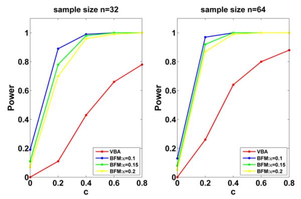
Simulation study: power of the local hypothesis tests for the effects of gestational age on FA and MD along the right internal capsule tract, under VBA and BFM, evaluated at five different values of c and three different values of for BFM, for sample sizes of 32 and 64 subjects.

We analyzed each simulation scenario by using 100 repeated simulations. We set n = 32 and 64. We randomly chose 16 males and 16 females for n = 32 (or 32 males and 32 females for n = 64) from our clinical data and used their values of gender and gestational age to simulate the values of FA and MD along the right internal capsule tract. We assigned Ga(1,1) hyper priors for the hyperparameters α and γ, and Ga(2,1) priors on a₁ and a₂. We specified ν = 3 and chose 5log((K+1)pM) as the starting number of factors. The MCMC algorithm was run 100,000 iterations, with the first 20,000 samples discarded as burn-in. For each case, we observed rapid convergence and efficient mixing.

We conducted the local hypothesis testing of $H_0^{\left(m\right)}\left(d_t\right):\mid {\beta }_2^{\left(m\right)}\left(d_t\right)\mid \le ∊$ for each point d_t along the right internal capsule tract and the mth diffusion property against $H_1^{\left(m\right)}\left(d_t\right):\mid {\beta }_2^{\left(m\right)}\left(d_t\right)\mid >∊$. We specified ∊^* = 0.1,0.15 and 0.2 for $∊={∊}^{\ast }{\max }_{d_t\in [0,L]}\sqrt{\widehat{\mathrm{var}}\left({\widehat{\beta }}_2^{\left(m\right)}\left(d_t\right)\right)}$, where max_dt∈[0,L] $\sqrt{\widehat{\mathrm{var}}\left({\widehat{\beta }}_2^{\left(m\right)}\left(d_t\right)\right)}$ is the maximum posterior standard deviation of ${\widehat{\beta }}_2^{\left(m\right)}\left(d_t\right)$ for d_t∈[0,L]. We evaluated FDR for the local hypothesis testing procedure in the null case c(d_t) = 0 and the local alternative cases c(d_t) = 0.2,0.4,0.6, and 0.8, and its power in the local alternative cases c(d_t) = 0.2,0.4,0.6, and 0.8. For each simulation, the significance level for the local hypothesis testing procedure was set at α_T = 0.05, and100 replications were used to estimate the FDR and powers. Finally, to show that BFM outperforms the voxel based analysis (VBA), we fitted general linear model (GLM) to the simulated data at each grid point and used FDR with α_T = 0.05 to correct for multiple comparisons. In GLM, we assumed fixed effects ${\mathit{B}}^{\left(m\right)}\left(d_t\right)=\left({\beta }_0^{\left(m\right)}\right(d_t),{\beta }_1^{\left(m\right)}(d_t),{\beta }_2^{\left(m\right)}(d_t\left)\right)$ at each grid point. As a comparison, we also evaluated FDR and powers.

Clinical DTI fiber tract data

The DTI fiber tract data come from a clinical study approved by the Institute Review Board of the University of North Carolina at Chapel Hill. This large study was designed to investigate early brain development. Healthy infants less than 1-year old were recruited with written informed consents obtained from their parents before imaging acquisition. In our study, a total of 128 healthy full-term infants (75 males and 53 females) are included, whose mean gestational age at MR scanning is 298±17.6days (range: 262 to 433days). All infants were placed with efforts such that they slept comfortably inside the MR scanner and none of them was sedated during the imaging acquisition. They were fed and calmed to sleep on a warm blanket with suitable ear protection.

The device used to acquire all images is a 3T Allegra head only MR system (Siemens Medical Inc., Erlangen, Germany), featuring 40mT/m for the maximal gradient strength and 400mT/(m.ms) for the maximal slew rate. Every subject was scanned for contiguous slices with slice thickness of 2mm to cover the whole brain. Each slice was repeated 5 times such that an average was obtained to improve the signal-to-noise ratio. These acquired DTI images are obtained via a single shot EPI DTI sequence (TR/TE=5400/73ms) with eddy current compensation. Diffusion gradients were collected at six non-colinear directions: (1,0,1), (−1,0,1), (0,1,1), (0,1,−1), (1,1,0), and (−1,1,0), at the b-value level of 1000s/mm². The reference scan at the b-value of 0 was implemented to construct diffusion tensor matrices. The voxel resolution was set at isotropic 2mm, and the in-place field of view was set at 256mm in both directions.

The diffusion tensors were constructed using a weighted least square estimation method (Basser et al., 1994b; Zhu et al., 2007). We then processed all 128 DTI datasets using the image processing steps in the DTI atlas building and computed diffusion properties along all fiber tracts of interest. We focused on analyzing two tracts of interest including the splenium of the corpus callosum tract and the right internal capsule tract (Figs. 3(a) and 8(a)). We computed fractional anistropy (FA), mean diffusivity (MD), and the three eigenvalues of the diffusion tensors, denoted by λ₁≥λ₂≥λ₃, at each grid point on both tracts for each of the 128 subjects. FA denotes the inhomogeneous extent of local barriers to water diffusion, and MD measures the averaged magnitude of local water diffusion. The three eigenvalues of the diffusion tensor reflect the magnitude of water diffusivity along and perpendicular to the long axis of white matter fibers (Song et al., 2003).

Fig. 3.

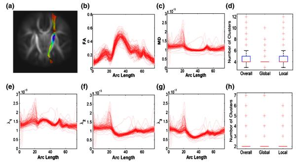
Right internal capsule tract description: (a) the right internal capsule tract extracted from the tensor atlas with color presenting mean FA value; diffusion properties of FA in panel (b), MD (mm²/s) in panel (c), λ₁ (mm²/s) in panel (e), λ₂ (mm²/s) in panel (f), λ₃ (mm²/s) in panel (g); the number of clusters posteriori in FA and MD trajectories in panel (d) and the number of clusters posteriori in λ₁, λ₂ and λ₃ trajectories in panel (h). The left-to-right direction of the arc corresponds to the superior-to-inferior direction of the right internal capsule tract.

Fig. 8.

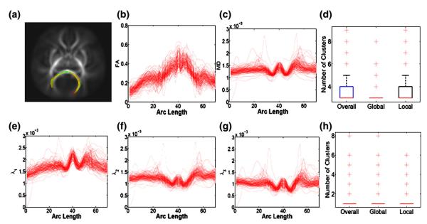
Splenium tract description: (a) the splenium capsule tract extracted from the tensor atlas with color presenting mean FA value; diffusion properties of FA in panel (b), MD (mm²/s) in panel (c), λ (mm² 1 /s) in panel (e), λ (mm² 2 /s) in panel (f), λ (mm² 3 /s) in panel (g); the number of clusters posteriori in FA and MD trajectories in panel (d) and the number of clusters posteriori in λ₁, λ₂ and λ₃ trajectories in panel (h). The left-to-right direction of the arc corresponds to the right-to-left direction of the splenium tract.

We focused on addressing four goals in the analysis of the multiple diffusion properties along the right internal capsule tract and the splenium tract. (i) Our first goal was to determine if there is a difference in the multiple diffusion properties along the fiber bundles between male and female infants. (ii) Our second goal was to investigate the development of the diffusion properties along the fiber bundles. (iii) Our third goal was to accomplish a parsimonious representation of the multiple diffusion trajectories across subjects. (iv) Our fourth goal was to examine covariate-dependent correlation patterns among the multiple diffusion properties along the fiber bundles.

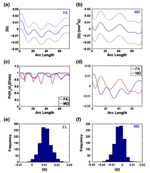
We applied BFM (9) to model the smoothed FA and MD functions (M = 2) along the right internal capsule and the splenium capsule with χ_i=(1,G_i,A_i)^T, where G_i and A_i refer to the gender (1 for female and 0 for male) and the gestational age of the ith infant. We estimated the ith subject’s varying coefficients ${\beta }_i^m\left(d_t\right)$ for the mth functional diffusion measure. We then estimated the mean coefficient curve ${\overline{\beta }}_k^{\left(m\right)}\left(d_t\right)$ a posteriori and constructed their 95% Bayesian credible bands from the posterior MCMC samples. We also empirically validated the pointwise posterior normality assumption for each ${\overline{\beta }}_k^{\left(m\right)}\left(d_t\right)$ by using the histogram of its posterior samples (Figs. 4(e) and (f)). We also performed local hypothesis testing procedures to determine if and where gender and gestational age are significantly associated with the diffusion measures along two fiber tracts. We conducted posterior cluster analysis to investigate the number of global and local clusters among the 128 infants in terms of the water diffusion properties FA and MD. We calculated the correlation analysis to illustrate the development of the correlation pattern between FA and MD along both fiber tracts for male infants at a mean gestational age of 298days, as well as the correlation pattern between the gestational age effects on FA and MD. Finally, we analyzed the three eigenvalues of diffusion tensors along the two fiber tracts.

Fig. 4.

Results of the gender effects on FA and MD along the right internal capsule tract: the estimated coefficient curves (–) and the corresponding 95% credible bands (- -) for FA in panel (a) and MD in panel (b); (c) the posterior probability curves (–) in favor of the grid point-wise alternative hypotheses (- - is the rejecting threshold); (d) the estimated mean FA and MD; (e) histogram at arc length=0 for FA; (f) histogram at arc length=75 for MD.

We assigned Ga(1, 1) hyper priors for the hyperparameters α and γ, a Ga(0.1, 0.1) prior for the precision parameters ${\sigma }_f^{-2}$, and Ga(2, 1) priors on a₁ and a₂. We specified ν = 3 and a default choice of 5log((K+ 1 )pM) as the initialized number of factors. We recommend these settings as default values in other analyses of DTI fiber tract data. We summarized the 1000 posterior samples from the MCMC output after the burn-in of 4000 iterations. Additionally, to perform the local hypothesis testing, we collected 80,000 posterior samples after the burn-in of 20,000 samples. Using multiple chains with widely-distributed points, the proposed MCMC algorithm exhibits good rates of convergence and mixing and takes 519s per 100 iterations in Matlab 2010b on a Lenovo X61 laptop. We repeated the same MCMC algorithm for different hyper-parameter values. For instance, we multiplied the mean and variance of α and γ by 2 and 0.5, and multiplied the variance of P₀ by 2 and 0.5. We used ν = 3.5,4, and 5 and varied b_σ between 0.1 and 0.5. We also used different starting numbers of factors between 3 and 10. The posterior results were found to be robust to the varying hyper-parameter values.

Results

Monte Carlo simulations

In the null case, FDR equals one based on its definition. Table 1 indicates that FDR is accurate for the sample size of 32 and 64. Consistent with our expectation, the statistical power for rejecting the local null hypotheses increases with the sample size and decreases with the zero neighborhood size ε. Inspecting Table 1 and Fig. 2 reveals that BFM is much more powerful than VBA. BFM has an attractive feature in explicitly modeling the structured inter-subject variability. In contrast, GLM used in VBA ignores the correlation among the tract data at different grid points, and thus the larger covariance estimates obtained from GLM decreases its power in signal detection.

Table 1.

Simulation study: FDR and power of the local hypothesis tests for the effects of gestational age on FA and MD along the right internal capsule tract under VBA and BFM

n	c	VBA		BFM
		FDR	Power	∊ = 0.1		∊ = 0.15		∊ = 0.2
				FDR	Power	FDR	Power	FDR	Power
32	0	1.00	0.00	1.00	0.19	1.00	0.11	1.00	0.07
	0.2	0.00	0.11	0.05	0.89	0.05	0.78	0.05	0.70
	0.4	0.00	0.43	0.02	0.99	0.03	0.98	0.03	0.96
	0.6	0.00	0.66	0.01	1.00	0.02	1.00	0.02	0.99
	0.8	0.00	0.78	0.01	1.00	0.01	1.00	0.02	1.00
64	0	1.00	0.00	1.00	0.13	1.00	0.08	1.00	0.05
	0.2	0.00	0.26	0.04	0.97	0.04	0.92	0.04	0.87
	0.4	0.00	0.64	0.01	1.00	0.02	1.00	0.02	0.99
	0.6	0.00	0.80	0.01	1.00	0.01	1.00	0.01	1.00
	0.8	0.00	0.88	0.01	1.00	0.01	1.00	0.01	1.00

Clinical DTI data: right internal capsule tract

Gender effects for FA and MD trajectories

Fig. 4(c) shows that the degrees of both FA and MD vary significantly between male and female groups along sub-regions of the right internal capsule (RIC) tract. Inspecting the posterior mean effect curves of gender on FA and MD and their 95% credible bands Figs. 4(a) and (b) reveal that in a large subregion of the RIC tract, FAs in female infants are smaller than those in male infants, whereas female infants have larger MD than male infants in half of the RIC tract, but such differences diminish in the other half of the RIC tract. The difference in MD between male and female groups was also observed in the sample average MD values (Fig. 4(d)). Such region-dependent differences between males and females were not observed by using FRATS and FADTTS. BFM has an advantage in modeling structured subject specific effects of gender, while FRATS and FADTTS assume identical gender effects for all subjects. The covariance estimates of FRATS and FADTTS are larger than the posterior variability of the posterior gender effect estimates of BFM. Therefore, FRATS and FADTTS are less powerful than BFM in detecting the gender effects which vary on tract regions.

Age related effects for FA and MD trajectories

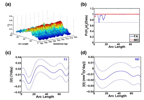
Similar to FRATS and FADTTS, Fig. 5(b) reveals uniformly significant gestational age effects on FA and MD values along the RIC tract. We also observed that FA increases with gestational age (Figs. 5(a) and (c)), while MD decreases with gestational age (Fig. 5(d)). This finding is consistent with the existing findings in other infant groups (McGraw et al., 2002).

Fig. 5.

Results of the gestational age effects on FA and MD along the right internal capsule tract: (a) 3D surf plot of FA along the right internal capsule tract for visualizing the gestational age effects; (b) the posterior probability curves (–) in favor of the grid point-wise alternative hypotheses (- - is the rejecting threshold); the estimated coefficient curves (–) and the corresponding 95% credible bands (- -) for FA in panel (c) and MD in panel (d).

Therefore, BFM provides a more advanced analytic approach to study the spatiotemporal trend in anisotropic development in new born infants. Latent clusters for FA and MD trajectories. We examined latent clusters in the FA and MD measures along the RIC tract across the 128 infants. The estimated value of the hyperparameter γ, controlling allocation weight on the local family, equals to 0.51 with 95% credible interval of [0.12, 1.20]. It implies that the posterior proportion of local clustering is 1/3, indicating that the data favors global clustering of the FA and MD trajectories across infants. The estimated value of the hyper-parameter α = 5.34, with 95% credible interval of [2.59, 9.65]. These values suggest few clusters. This conclusion is further supported by the estimated values of 4.45, 3.94, and 4.42 for the numbers of overall, global, and local clusters, respectively (Fig. 3(d)). This result agrees with the FA and MD trajectories in Figs. 5(b) and (c). For instance, although most MD trajectories cluster together, some ‘outlying’ MD trajectories exist with extremely smaller/larger MD values.

Gender and age-dependent correlation patterns for FA and MD trajectories

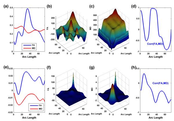
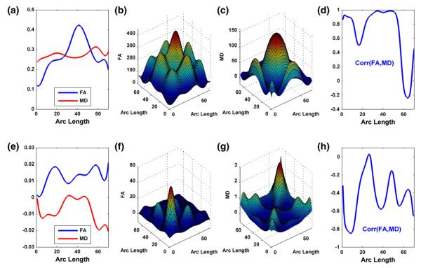
Along the RIC tract, we further computed the posterior mean curves of FA and MD (Fig. 6(a)) for male infants at the mean gestational age and estimated their posterior covariance matrices (Figs. 6(b) and (c)). We observed the pattern of oscillating between positive and negative correlations with negative correlations at around 60% of grid points (Fig. 6(d)). It agrees with the gender effects on FA and MD trajectories in Fig. 4(d). We also computed the posterior covariance matrices for the gestational age effects on FA and MD values (Figs. 6(f) and (g)) and derived the grid pointwise correlation between the gestational age effects on FA and MD. Fig. 6(h) reveals negative correlations at most grid points. It agrees with the ‘opposite’ development patterns of FA and MD trajectories with gestational age (Figs. 5(a), (c), and(d)).

Fig. 6.

Results from the analysis of FA and MD (mm²/s) along the right internal capsule tract: (a) the posterior estimated curves of FA and MD for male infants at the mean gestational age; the estimated covariance matrices for FA in panel (b) and MD in panel (c) for male infants at the mean gestational age; (d) the estimated correlations between FA and MD for male infants at the mean gestational age; (e) the posterior estimated gestational age effects; the estimated covariance matrices for the gestational age effects on FA in panel (f) and MD in panel (g); (h) the estimated correlations between the gestational age effects on FA and MD.

Results based on eigenvalue trajectories

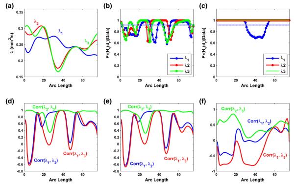
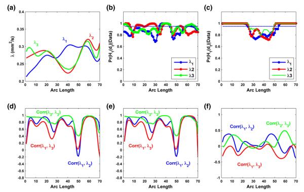
In the analysis of the three eigenvalues, a similar locally significant pattern of gender effect was observed for all three eigenvalues (Fig. 7(b)). Gestational age effect was found uniformly significant for λ₂ and λ₃, while locally head-and-tail significant for λ₁ (Fig. 7(c)). We observed positive correlations between λ₂ and λ₃ for both male and female groups at the mean gestational age (Figs. 7(d) and (e)), and positive correlation between the gestational age effects on λ₂ and λ₃ (Fig. 7(f)). Overall, these correlations between λ₂ and λ₃ are larger than those between λ₁ and λ₃ or λ₁ and λ₂. It agrees with the small differences between λ₂ and λ₃ and the relatively large differences between λ₁ and λ₃ or λ₁ and λ₂ in the middle of the RIC tract (Figs. 3(e), (f) and (g)). Finally, the cluster analysis of the three eigenvalues along the RIC tract across all infants reveals small numbers of overall, global, and local clusters (Fig. 3(h)).

Fig. 7.

Results from the analysis of the three eigenvalues of diffusion tensor on the right internal capsule tract: (a) the estimated mean functions for λ₁ (blue), λ₂ (red) and λ₃ (green); the posterior probability curves (–) in favor of the grid point-wise alternative hypotheses for the gender effects in panel (b) and the gestational age effects in panel (c) (- - is the rejecting threshold); the estimated correlations among λ₁, λ₂ and λ₃ for male infants at the mean gestational age in panel (d) and female infants at the mean gestational age in panel (e), and among the gestational age effects on λ₁, λ₂ and λ₃ in panel (f).

Clinical DTI data: splenium tract

Gender and age effects for FA and MD trajectories

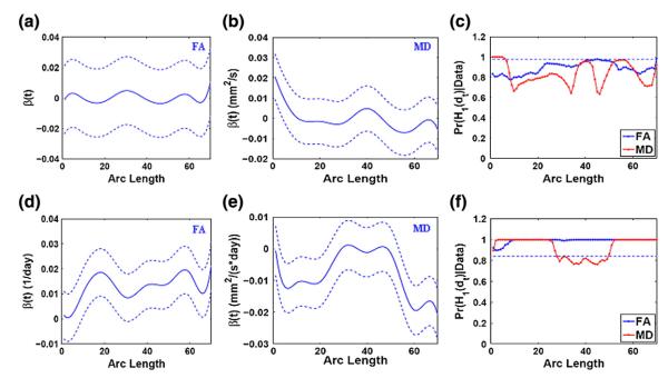
Fig. 9(c) shows that gender is only slightly significant for MD development in the head subregion of the splenium tract. The posterior estimates for the mean effects of gender and the corresponding 95% credible bands agree with the testing results. Figs. 9(d)–(e) display the uniformly increasing effects of gestational age on FA development and decreasing effects on MD development at a major subregion of the splenium tract. The local hypothesis testing results (Fig. 9(f)) support that gestational age is uniformly significant along the splenium tract for the developmental change of FA, but locally significant for MD.

Fig. 9.

Results from the analysis of FA and MD along the splenium tract: the estimated coefficient curves (–) and the corresponding 95% credible bands (- -) for the gender effects (panel (a) for FA and panel (b) for MD) and the gestational age effects (panel (d) for FA and panel (e) for MD); the posterior probability curves (–) in favor of the grid point-wise alternative hypotheses for the gender effects (panel (c)) and the gestational age effects (panel (f)) (- - is the rejecting threshold).

Latent clusters for FA and MD trajectories

Fig. 8(d) shows the posterior sampling distribution of the number of clusters among the 128 infants. The posterior mean estimates of the numbers of overall, global, and local clusters are 3.42, 3.07, and 3.40, respectively, indicating that the 128 infants concentrate on a few clusters. The weight parameter γ for allocation on the local family was estimated to be 0.38 with 95% credible interval of [0.08, 0.98]. The estimated posterior mean of the proportion of local clustering is 0.28, which favors a global clustering of all infants. The estimated posterior mean of α equals to 6.46, with 95% credible interval of [2.94, 11.80]. This result agrees with the sparse clusters identified in the data (Fig. 8(b), (c), (e), (f), and (g)). For instance, variation in FA and MD trajectories is relatively high with some ‘outlying’ trajectories.

Gender and Age-dependent correlation patterns for FA and MD trajectories

Figs. 10(a)–(c) present the posterior estimation of the mean curves of FA and MD for male infants at the mean gestational age and the posterior estimates of their covariance matrices. Inspecting Fig. 10(d) reveals that male infants at the mean gestational age have positive correlations between FA and MD at a major subregion of the splenium tract. Furthermore, Figs. 10(e)–(g) present the estimated curves associated with gestational age effects and their corresponding covariance matrices. We observed that the gestational age effects on FA and MD are negatively correlated almost along the whole splenium tract (Fig. 10(h)), which is consistent with the opposite trend of gestational age on FA and MD values along the splenium tract (Fig. 10(e)).

Fig. 10.

Results from the analysis of FA and MD (mm²/s) along the splenium tract: (a) the posterior estimated curves of FA and MD for male infants at the mean gestational age; the estimated covariance matrices for FA in panel (b) and MD in panel (c) for male infants at the mean gestational age; (d) the estimated correlations between FA and MD for male infants at the mean gestational age; (e) the posterior estimated gestational age effects; the estimated covariance matrices for the gestational age effects on FA in panel (f) and MD in panel (g); (h) the estimated correlations between the gestational age effects on FA and MD.

Results based on eigenvalue trajectories

We also observed that both gender and gestational age are locally significantly associated with the developmental patterns of the three eigenvalues along the splenium tract (Figs. 11(b) and (c)). We further observed large correlation between λ₂ and λ₃ and relatively weak correlation between λ₁ and λ₂ or λ₁ and λ₃ for both male and female groups at the mean gestational age. This agrees with the small difference between λ₂ and λ₃, but relatively large difference between λ₁ and λ₃ in the first half subregion of the splenium tract (Figs. 8(e), (f) and (g)). We did not observe noticeable difference among the pairwise correlations of the gestational age effects on the three eigenvalues (Fig. 11(f)).

Fig. 11.

Results from the analysis of the three eigenvalues of diffusion tensor on the splenium tract: (a) the estimated mean functions for λ₁ (blue), λ₂ (red) and λ₃ (green); the posterior probability curves (–) in favor of the grid point-wise alternative hypotheses for the gender effects in panel (b) and the gestational age effects in panel (c) (- - is the rejecting threshold); the estimated correlations among λ₁, λ₂ and λ₃ for male infants at the mean gestational age in panel (d) and female infants at the mean gestational age in panel (e), and among the gestational age effects on λ₁, λ₂ and λ₃ in panel (f).

Discussion

A prior study is particularly relevant to the present study, because it examined the anisotropic trend across three age groups in infants (McGraw et al., 2002). Our results on the association between anisotropic values and gestational age agree with their findings with a few key differences. We identified the association of anisotropic values with gestational age changing over the brain regions. The region-dependent association is evaluated on the basis of integrative multivariate diffusion properties rather than univariate anisotropic outcome in McGraw et al. (2002). The region-dependent association reveals the complex inhomogeneous spatio-temporal maturation patterns of fiber bundle diffusion properties in infant nerve development. Hence, BFM presents a novel robust analytic approach to capture complex spatio-temporal pattern of diffusion properties in infant nerve structure.

From the statistical perspective, we have developed a new Bayesian functional analysis pipeline BFM for delineating the structure of the variability of multiple diffusion properties along major white matter fiber bundles and their association with a set of covariates of interest. The BFM pipeline integrates five advanced Bayesian statistical tools from the statistical literature. Compared with the existing literature (Zhu et al., 2010, 2011), our BFM explicitly models subject-specific functional covariate effects on the multiple diffusion outcome functions and the covariate-specific correlation structure among the multiple diffusion measures. From the application perspective, we have demonstrated BFM in a clinical study of neurodevelopment. Our results have revealed the complex inhomogeneous spatio-temporal maturation patterns of fiber bundle diffusion properties. Our BFM not only boosts the statistical power in detecting signal of interest, but also improves prediction accuracy, which is very important for real applications.

Several limitations need to be addressed in future research. First, since the existing fiber tract based methods including BFM require DTI fiber correspondence across subjects, BFM cannot be used to investigate some scenarios in practice. For instance, it is possible that the centroid of the localization of white matter lesion may vary across time and subjects. In this case, one cannot use both ROI-based methods and tract based methods. Secondly, although we have used the B-spline basis functions in BFM, it is interesting to consider other basis functions, such as wavelets. Thirdly, since diffusion properties may be non-normally distributed, it is interesting to consider other distributions for the measurement error. Fourthly, BFM is limited to diffusion properties along fiber bundle, but it is interesting to consider full DTs and other representations based on high angular resolution diffusion image (HARDI) (Lenglet et al., 2009; Lepore et al., 2008; Schwartzman; Schwartzman et al., 2005; Tuch et al., 2002; Whitcher et al., 2007; Zhu et al., 2009). Fifthly, BFM can be readily extended to more complex brain structures, such as the medial manifolds of fiber tracts (Yushkevich et al., 2008), functional neuroimaging data (DuBois Bowman et al., 2008; Gössl et al., 2001; Woolrich et al., 2004; Xu et al., 2009), and group analysis of neuroimaging data (Penny et al., 2007; Rosa et al., 2010).

Appendix A. Posterior computation

We develop an efficient Markov chain Monte Carlo (MCMC) algorithm for posterior computation. After truncating the loadings matrix A to h^*⪡(K + 1) pM columns, we adapt an efficient slice sampling Gibbs sampler (Kalli et al., 2011; Papaspiliopoulos, 2008) for mixture models. This Gibbs sampler combines the advantages of the retrospective MCMC method (Papaspiliopoulos and Roberts, 2008) and the slice sampling method (Walker, 2007). It introduces auxiliary variables to avoid truncated approximations. This algorithm is straightforward to implement and exhibits good performance in convergence and mixing. We will describe the adaptation strategy on the truncated level h^* after introducing the Gibbs sampler.

Allowing data to inform information about the hyperparameters involved in the model through Eqs. (1)–(7), we specify α~Ga(a_α,b_α) and γ~Ga(a_γ,b_γ). Introducing auxiliary variables u={u_ih:i = 1,…,n; h = 0,1,…,h^*} to avoid truncated approximations, the complete data joint likelihood of y, u and z is:

$$\prod _{i=1}^n\mathsf{g}({\mathit{Y}}_i;\mathit{A},{\theta }_{{\psi }_i},\Sigma )1\left(u_{i0}<{\pi }_{{\psi }_{i0}}\right)\prod _{h=1}^{h^{\ast }}1\left(u_{\mathit{ih}}<{\pi }_{{\psi }_{\mathit{ih}}}\right){\nu }_h^{z_{\mathit{ih}}}{(1-{\nu }_h)}^{1-z_{\mathit{ih}}},$$

where Y_i is a ${\Sigma }_{m=1}^M{n}_{m_i}\times 1$ outcome vector for the M measures of the ith subject, g(·) is the density function of the outcome vector Y_i, i = 1,…,n, and the elements in u are constrained to the interval (0, 1).

Starting from the initiation step, the Gibbs sampler at the truncated level h^* proceeds as follows:

1. Update the hth column of the factor loadings matrix A_h^*, denoted by A_h, from its conditional distribution

   $$p({\mathit{A}}_h\mid -)~\mathit{N}\left({\left({\mathit{C}}_{\mathit{h}}^{\mathit{T}}{\Sigma }_N^{-1}{\mathit{C}}_h+{\Sigma }_{A_h}^{-1}\right)}^{-1}{\mathit{C}}_h^T{\Sigma }_N^{-1}{Y}_h,{\left({\mathit{C}}_h^T{\Sigma }_N^{-1}{\mathit{C}}_h+{\Sigma }_{A_h}^{-1}\right)}^{-1}\right),$$

   where ${\mathit{Y}}_h={({\mathit{Y}}_{1h}^T,\dots ,{\mathit{Y}}_{\mathit{nh}}^T)}^T$ with ${\mathit{Y}}_{\mathit{ih}}={\mathit{Y}}_i-{\Sigma }_{j\ne h}{\mathit{I}}_M\otimes {\mathit{B}}_i{\mathit{A}}_j{\theta }_{{\Psi }_m\mathit{iij}}$, ${\mathit{C}}_h=\left(\begin{array}{c}\hfill {\theta }_{{\psi }_{1h}}({\mathit{I}}_M\otimes {\mathit{B}}_1)\hfill \\ \hfill ⋮\hfill \\ \hfill {\theta }_{{\psi }_{\mathit{nh}}}({\mathit{I}}_M\otimes {\mathit{B}}_1)\hfill \end{array}\right),\text{and}{\Sigma }_N={\mathit{I}}_n\otimes \Sigma ,{\Sigma }_{A_h}=\text{diag}({\varphi }_{1,h}^{-1}{\tau }_h^{-1},\dots ,{\varphi }_{(K+1)\mathit{pM},h}^{-1}{\tau }_h^{-1}\text{for}h=1,\dots ,h^{\ast }$
2. Update ϕ_gh from its conditional distribution

   $$p({\varphi }_{\mathit{gh}}\mid -)~\mathrm{Ga}\left(\frac{v+1}{2},\frac{v+A_{\mathit{gh}}^2{T}_h}{2}\right).$$
3. Update δ₁ from its conditional distribution

   $$p({\delta }_1\mid -)~\mathrm{Ga}\left(a_1+\frac{1}{2}(K+1){\mathit{pMh}}^{\ast },1+\frac{1}{2}\sum _{h=1}^{h^{\ast }}{\tau }_h^{\left(1\right)}\sum _{g=1}^{(K+1)\mathit{pM}}{\varphi }_{\mathit{gh}}{A}_{\mathit{gh}}^2\right),$$

   and update δ₁, l≥2 from its conditional distribution

   $$p({\delta }_l\mid -)~\mathrm{Ga}\left(a_2+\frac{1}{2}(K+1)\mathit{pM}(h^{\ast }-l+1),1+\frac{1}{2}\sum _{h=1}^{h^{\ast }}{\tau }_h^{\left(l\right)}\sum _{g=1}^{(K+1)\mathit{pM}}{\varphi }_{\mathit{gh}}{A}_{\mathit{gh}}^2\right),$$

   where ${\tau }_h^{\left(l\right)}={\prod }_{t=1,h\ne l}^h{\delta }_t,l=1,\dots ,h^{\ast }$
4. Update ${\sigma }_f^{-2}$, f = 1,…,MT, from its conditional distribution

   $$p({\sigma }_f^{-2}\mid -)~\mathrm{Ga}\left(a_{\sigma }+\frac{n}{2},b_{\sigma }+\frac{1}{2}\sum _{i=1}^n{\left(y_{\mathit{if}}-{({\mathit{I}}_M\otimes {\mathit{B}}_i)}_f\mathit{A}{\theta }_{{\psi }_i}\right)}^2\right),$$

   where (I_M⊗B_i)_f denotes the fth row of (I_M⊗B_i).
5. Update u_ih from its conditional distribution

   $$p(u_{\mathit{ih}}\mid -)~\text{Unif}(0,{\pi }_{{\psi }_{\mathit{ih}}}).$$
6. Update the latent z_ih from its conditional distribution

   $$p(z_{\mathit{ih}}\mid -)~\text{Ber}\left(\frac{{\nu }_{h}N({\mathit{Y}}_i;\mathit{A},{\theta }_{i(z_{\mathit{ih}}=1),}\Sigma )}{{\nu }_{h}N\left({\mathit{Y}}_i;\mathit{A},{\theta }_{i(z_{\mathit{ih}}=1),}\Sigma \right)+(1-{\nu }_h)N\left({\mathit{Y}}_i;\mathit{A},{\theta }_{i(z_{\mathit{ih}}=0),}\Sigma \right)}\right),$$

   where θ_{i(zih = j)} refers to the current value of θ_i with inserting θ_0ϕi0h to the hth component for j = 1, and θ_0ϕi0h for j = 0.
7. Update the stick-breaking weights ${\pi }_q^{\ast }$ from its conditional distribution

   $$p({\pi }_q^{\ast }\mid -)~\text{Beta}\left(\sum _{h=0}^{h^{\ast }}\sum _{i=1}^{n}1({\psi }_{\mathit{ih}}=q)+1,\sum _{h=0}^{h^{\ast }}\sum _{i=1}^{n}1\left({\psi }_{\mathit{ih}}>q\right)+\alpha \right),$$

   for q≤ψ^* with ψ^* = max{ψ_ih:i = 1, …,nh = 0.1,…,h^*], for q≤ψ^*, sample ${\pi }_q^{\ast }$ from $p({\pi }_q^{\ast }\mid -)$ ~ Beta(1, α)
8. Update the allocation index ψ_ih, from its conditional distribution

   $$\mathit{P}({\psi }_{\mathit{ih}}=q\mid -)\propto 1(q\in C_{\pi }(u_{\mathit{ih}}\left)\right)N({\mathit{Y}}_i;\mathit{A},{\theta }_{{\psi }_{\mathit{ih}}=q}\Sigma ),$$

   where C_π(u_ih) = {q:π_q>u_ih}⊂{1,2,…,∞}, and ${\pi }_q^{\ast }$ is sampled for q = 1, …,$q=1,\dots ,\tilde{\psi }$ such that

   $$\sum _{q=1}^{\tilde{\psi }}{\pi }_q^{\ast }\prod _{l\le q}(1-{\pi }_l^{\ast })\ge 1-u^{\ast },$$

   where u^* = min{u_ih:i =1,…n,h = 0,1,…,h*}.
9. Update θ_jq from its conditional distribution

   $$p({\theta }_{\mathit{jq}}\mid -)~{\mathit{N}}_{h^{\ast }}({\left[\text{diag}\left(1_{h^{\ast }}{\zeta }_{\mathit{jq}}\right)+{\mathit{W}}_{\mathit{jq}}^{\prime }{\Sigma }_N^{-1}{\mathit{W}}_{\mathit{jq}}\right]}^{-1}{\mathit{W}}_{\mathit{jq}}^{\prime }{\Sigma }_N^{-1}{\mathit{Y}}_{\mathit{jq}},\left[\text{diag}\left(1_{h^{\ast }}{\zeta }_{\mathit{jq}}\right)+{\mathit{W}}_{\mathit{jq}}^{\prime }{\Sigma }_N^{-1}{\mathit{W}}_{\mathit{jq}}\right]-1),$$

   in which Y_jq refers to the contribution for θ_jq from subjects with z_ih = 1 – j and ϕ_ih = q. In addition, W_jq = diag(w₁,…,w_n)ZΦR and Y_jq = diag(Y₁,…,Y_n)Z_YΦ_Y1_n, where

   • w_i = I_M⊗B_iA,
   • Z = Blkdiag(Z₁,…,Z_n) with Z_i = diag(1(z_i1 = 1–j),…,1(z_ih^* = 1–j)),
   • Φ = Blkdiag(Φ₁,…,Φ_n) with Φ_i = diag(1(ψ_i1 = q),…,1(ψ_ih* = q)),
   • R = 1_n⊗I_h*,
   • Z_Y = Blkdiag(Z_Y1,…,Z_Yn) with $Z_{\mathit{Yi}}=1\left({\Sigma }_{h=1}^{h^{\ast }}1\right(z_{\mathit{ih}}=1-j)\ge 1)$,
   • Φ_Y = Blkdiag(Φ_Y1,…,Φ_Yn) with ${\Phi }_{Y_i}=1\left({\Sigma }_{h=1}^{h^{\ast }}1\right({\psi }_{\mathit{ih}}=q)\ge 1)$,
   • and 1_n is a n × 1 vector of entries of 1.

10. Update ζ_jq from its conditional distribution Ga(0.5+h*/2,0.5+θ_jqθ_jq/2).

11. Update the hyperparameter γ from its conditional distribution Ga($(a_{\gamma }+h^{\ast },b_{\gamma }-{\Sigma }_{h=1}^{h^{\ast }}\log (1-{\nu }_h\left)\right)$).

12. Update the hyperparameter α from its conditional distribution Ga($(a_{\alpha }+{\psi }^{\ast },b_{\alpha }-{\Sigma }_{q=1}^{{\psi }^{\ast }}\log (1-{\pi }_q^{\ast }\left)\right)$).

To choose the effective number of factors, we use an adaptation approach (Bhattacharya and Dunson, 2011) to update the truncated number of factors h^* across iterations. Starting with a conservative guess h^* of h^*, we adapt with probability p(t)=exp(α₀+α₁t) at the tth iteration. We specify α₀ and α₁ such that the chain comes with adaptation around every 10 iterations at the beginning and exponentially fast decreasing in adaptation frequency. In detail, at the tth iteration, we monitor the columns in the factor loadings by comparing u_t with p(t), where u_t is a sequence randomly generated from Unif(0, 1). If u_t≤p(t), we remove the columns having all elements within some pre-specified small zero neighborhood, called redundant columns, and retain non-redundant columns for other parameters. If no such redundant column is detected, we add a new column to the loadings, and sample other parameters from their prior distributions to fill in the additional columns.

References

- Ashburner J, Friston KJ. Voxel-based morphometry: the methods. Neuroimage. 2000;11:805–821. doi: 10.1006/nimg.2000.0582. [DOI] [PubMed] [Google Scholar]
- Basser PJ, Mattiello J, LeBihan D. Estimation of the effective self-diffusion tensor from the NMR spin echo. J. Magn. Reson. 1994a;103:247–254. doi: 10.1006/jmrb.1994.1037. [DOI] [PubMed] [Google Scholar]
- Basser PJ, Mattiello J, LeBihan D. MR diffusion tensor spectroscopy and imaging. Biophys. J. 1994b;66:259–267. doi: 10.1016/S0006-3495(94)80775-1. [DOI] [PMC free article] [PubMed] [Google Scholar]
- Bhattacharya A, Dunson DB. Sparse Bayesian infinite factor models. Biometrika. 2011;98(2):291–306. doi: 10.1093/biomet/asr013. [DOI] [PMC free article] [PubMed] [Google Scholar]
- Bonekamp D, Nagae LM, Degaonkar M, Matson M, Abdalla WM, Barker PB, Mori S, Horská A. Diffusion tensor imaging in children and adolescents: reproducibility, hemispheric, and age-related differences. Neuroimage. 2008;34:733–742. doi: 10.1016/j.neuroimage.2006.09.020. [DOI] [PMC free article] [PubMed] [Google Scholar]
- Camara E, Bodammer N, Rodriguez-Fornells A, Tempelmann C. Age-related water diffusion changes in human brain: a voxel-based approach. Neuroimage. 2007;34:1588–1599. doi: 10.1016/j.neuroimage.2006.09.045. [DOI] [PubMed] [Google Scholar]
- Carvalho CM, Chang J, Lucas JE, Nevins JR, Wang Q, West M. High-dimensional sparse factor modeling: applications in gene expression genomics. J. Am. Stat. Assoc. 2008;103(484):1438–1456. doi: 10.1198/016214508000000869. [DOI] [PMC free article] [PubMed] [Google Scholar]
- Cascio CJ, Gerig G, Piven J. Diffusion tensor imaging: application to the study of the developing brain. J. Am. Acad. Child Adolesc. Psychiatry. 2007;46:213–223. doi: 10.1097/01.chi.0000246064.93200.e8. [DOI] [PubMed] [Google Scholar]
- Chen YS, An HY, Zhu HT, Stone T, Smith JK, Hall C, Bullitt E, Shen DG, Lin WL. White matter abnormalities revealed by diffusion tensor imaging in non-demented and demented HIV+ patients. Neuroimage. 2009;47:1154–1162. doi: 10.1016/j.neuroimage.2009.04.030. [DOI] [PMC free article] [PubMed] [Google Scholar]
- Crainiceanu CM, Ruppert D, Carroll RJ, Joshi A, Goodner B. Spatially adaptive Bayesian penalized splines with heteroscedastic errors. J. Comput. Graph. Stat. 2007;16(2):265–288. [Google Scholar]
- DuBois Bowman F, Caffo B, Bassett SS, Kilts C. A Bayesian hierarchical framework for spatial modeling of fMRI data. Neuroimage. 2008;39(1):146–156. doi: 10.1016/j.neuroimage.2007.08.012. [DOI] [PMC free article] [PubMed] [Google Scholar]
- Dunson DB. Nonparametric Bayes local partition models for random effects. Biometrika. 2009;96:249–262. doi: 10.1093/biomet/asp021. [DOI] [PMC free article] [PubMed] [Google Scholar]
- Ferguson TS. A Bayesian analysis of some nonparametric problems. Ann. Stat. 1973;1(2):209–230. [Google Scholar]
- Ferguson TS. Prior distributions on spaces of probability measures. Ann. Stat. 1974;2(4):615–629. [Google Scholar]
- Focke NK, Yogarajah M, Bonelli SB, Bartlett PA, Symms MR, Duncan JS. Voxel-based diffusion tensor imaging in patients with mesial temporal lobe epilepsy and hippocampal sclerosis. Neuroimage. 2008;40:728–737. doi: 10.1016/j.neuroimage.2007.12.031. [DOI] [PubMed] [Google Scholar]
- Geweke J, Zhou G. Measuring the pricing error of the arbitrage pricing theory. Rev. Financ. Stud. 1996;9(2):557–587. [Google Scholar]
- Gilmore JH, Smith LC, Wolfe HM, Hertzberg BS, Smith JK, Chescheir NC, Evans DD, Kang C, Hamer RM, Lin W, Gerig G. Prenatal mild ventriculomegaly predicts abnormal development of the neonatal brain. Biol. Psychiatry. 2008;64:1069–1076. doi: 10.1016/j.biopsych.2008.07. [DOI] [PMC free article] [PubMed] [Google Scholar]
- Goldsmith A, Feder J, Crainiceanu C, Caffo B, Reich D. Penalized functional regression. J. Comput. Graph. Stat. 2011;20:830–851. doi: 10.1198/jcgs.2010.10007. [DOI] [PMC free article] [PubMed] [Google Scholar]
- Goodlett CB, Fletcher PT, Gilmore JH, Gerig G. Group analysis of DTI fiber tract statistics with application to neurodevelopment. Neuroimage. 2009;45:S133–S142. doi: 10.1016/j.neuroimage.2008.10.060. [DOI] [PMC free article] [PubMed] [Google Scholar]
- Gössl C, Auer DP, Fahrmeir L. Bayesian spatiotemporal inference in functional magnetic resonance imaging. Biometrics. 2001;57(2):554–562. doi: 10.1111/j.0006-341x.2001.00554.x. [DOI] [PubMed] [Google Scholar]
- Greven S, Crainiceanu C, Caffo B, Reich D. Longitudinal functional principal component analysis. Electron. J. Stat. 2010;4:1022–1054. doi: 10.1214/10-EJS575. [DOI] [PMC free article] [PubMed] [Google Scholar]
- Hasan KM, Basser PJ, Parker DL, Alexander AL. Analytical computation of the eigenvalues and eigenvectors in DT-MRI. J. Magn. Reson. 2001;152:41–47. doi: 10.1006/jmre.2001.2400. [DOI] [PubMed] [Google Scholar]
- Hasan KM, Narayana PA. Computation of the fractional anisotropy and mean diffusivity maps without tensor decoding and diagonalization: theoretical analysis and validation. Magn. Reson. Med. 2003;50:589–598. doi: 10.1002/mrm.10552. [DOI] [PubMed] [Google Scholar]
- Jeffreys W, Berger J. Ockham’s razor and Bayesian analysis. Am. Stat. 1992;80:64–72. [Google Scholar]
- Jones DK, Symms MR, Cercignani M, Howard RJ. The effect of filter size on VBM analyses of DT-MRI data. Neuroimage. 2005;26:546–554. doi: 10.1016/j.neuroimage.2005.02.013. [DOI] [PubMed] [Google Scholar]
- Kalli M, Griffin J, Walker S. Slice sampling mixture models. Stat. Comput. 2011;21:93–105. [Google Scholar]
- Kubicki M, McCarley R, Westin CF, Park HJ, Maier S, Kikinis R, Jolesz FA, Shenton ME. A review of diffusion tensor imaging studies in schizophrenia. J. Psychiatr. Res. 2007;41(1–2):15–30. doi: 10.1016/j.jpsychires.2005.05.005. [DOI] [PMC free article] [PubMed] [Google Scholar]
- Lenglet C, Campbell JSW, Descoteaux M, Haro G, Savadjiev P, Wassermann D, Anwander A, Deriche R, Pike GB, Sapiro G, Siddiqi K, Thompson PM. Mathematical methods for diffusion MRI processing. Neuroimage. 2009;45:S111–S122. doi: 10.1016/j.neuroimage.2008.10.054. [DOI] [PMC free article] [PubMed] [Google Scholar]
- Lepore N, Brun CA, Chou Y, Chiang M, Dutton RA, Hayashi KM, Luders E, Lopez OL, Aizenstein HJ, Toga AW, Becker JT, Thompson PM. Generalized tensor-based morphometry of HIV/AIDS using multivariate statistics on deformation tensors. IEEE Trans. Med. Imaging. 2008;27:129–141. doi: 10.1109/TMI.2007.906091. [DOI] [PMC free article] [PubMed] [Google Scholar]
- McGraw P, Liang L, Provenzale J. Evaluation of normal age-related changes in anisotropy during infancy and childhood as shown by diffusion tensor imaging. Am. J. Roentgenol. 2002;179:1515–1522. doi: 10.2214/ajr.179.6.1791515. [DOI] [PubMed] [Google Scholar]
- Moseley M. Diffusion tensor imaging and aging—a review. NMR Biomed. 2002;15:553–560. doi: 10.1002/nbm.785. [DOI] [PubMed] [Google Scholar]
- Mukherjee P, McKinstry RC. Diffusion tensor imaging and tractography of human brain development. Neuroimaging Clin. N. Am. 2006;16:19–43. doi: 10.1016/j.nic.2005.11.004. [DOI] [PubMed] [Google Scholar]
- Müller P, Parmigiani G, Robert C, Rousseau J. Optimal sample size for multiple testing: the case of gene expression microarrays. J. Am. Stat. Assoc. 2004;99:990–1001. [Google Scholar]
- O’Donnell L, Westin CF, Golby A. Tract-based morphometry for white matter group analysis. Neuroimage. 2009;45:832–844. doi: 10.1016/j.neuroimage.2008.12.023. [DOI] [PMC free article] [PubMed] [Google Scholar]
- Papaspiliopoulos O. A note on posterior sampling from Dirichlet mixture models. Tech. rep. Universitat Pompeu Fabra. 2008 [Google Scholar]
- Papaspiliopoulos O, Roberts G. Retrospective Markov chain Monte Carlo methods for Dirichlet process hierarchical models. Biometrika. 2008;95:169–186. [Google Scholar]
- Penny W, Kilner J, Blankenburg F. Robust Bayesian general linear models. Neuroimage. 2007;36:661–671. doi: 10.1016/j.neuroimage.2007.01.058. [DOI] [PubMed] [Google Scholar]
- Pierpaoli C, Basser PJ. Toward a quantitative assessment of diffusion anisotropy. Magn. Reson. Med. 1996;36:893–906. doi: 10.1002/mrm.1910360612. [DOI] [PubMed] [Google Scholar]
- Rollins NK. Clinical applications of diffusion tensor imaging and tractography in children. Pediatr. Radiol. 2007;37:769–780. doi: 10.1007/s00247-007-0524-z. [DOI] [PubMed] [Google Scholar]
- Rosa MJ, Bestmann S, Harrison L, Penny W. Bayesian model selection maps for group studies. Neuroimage. 2010;49(1):217–224. doi: 10.1016/j.neuroimage.2009.08.051. [DOI] [PMC free article] [PubMed] [Google Scholar]
- Schwartzman A. Ph.D. thesis. Stanford University; Random ellipsoids and false discovery rates: statistics for diffusion tensor imaging data. [Google Scholar]
- Schwartzman A, Dougherty RF, Taylor JE. Cross-subject comparison of principal diffusion direction maps. Magn. Reson. Med. 2005;53:1423–1431. doi: 10.1002/mrm.20503. [DOI] [PMC free article] [PubMed] [Google Scholar]
- Smith SM, Jenkinson M, Johansen-Berg H, Rueckert D, Nichols TE, Mackay CE, Watkins KE, Ciccarelli O, Cader M, Matthews P, Behrens TE. Tractbased spatial statistics: voxelwise analysis of multi-subject diffusion data. Neuroimage. 2006;31:1487–1505. doi: 10.1016/j.neuroimage.2006.02.024. [DOI] [PubMed] [Google Scholar]
- Snook L, Paulson LA, Roy D, Phillips L, Beaulieu C. Diffusion tensor imaging of neurodevelopment in children and young adults. Neuroimage. 2005;26:1164–1173. doi: 10.1016/j.neuroimage.2005.03.016. [DOI] [PubMed] [Google Scholar]
- Snook L, Plewes C, Beaulieu C. Voxel based versus region of interest analysis in diffusion tensor imaging of neurodevelopment. Neuroimage. 2007;34:243–252. doi: 10.1016/j.neuroimage.2006.07.021. [DOI] [PubMed] [Google Scholar]
- Song SK, Sun SW, Ju WK, Lin SJ, Cross AH, Neufeld AH. Diffusion tensor imaging detects and differentiates axon and myelin degeneration in mouse optic nerve after retinal ischemia. Neuroimage. 2003;20:1714–1722. doi: 10.1016/j.neuroimage.2003.07.005. [DOI] [PubMed] [Google Scholar]
- Stieltjes B, Kaufmann WE, van Zijl PC, Fredericksen K, Pearlson GD, Solaiyappan M, Mori S. Diffusion tensor imaging and axonal tracking in the human brainstem. Neuroimage. 2001;14(3):723–735. doi: 10.1006/nimg.2001.0861. [DOI] [PubMed] [Google Scholar]
- Tuch DS, Reese TG, Wiegell MR, Makris N, Belliveau JW, Wedeen VJ. High angular resolution diffusion imaging reveals intravoxel white matter fiber heterogeneity. Magn. Reson. Med. 2002;48:577–582. doi: 10.1002/mrm.10268. [DOI] [PubMed] [Google Scholar]
- Van Hecke W, Sijbers J, De Backer S, Poot D, Parizel PM, Leemans A. On the construction of a ground truth framework for evaluating voxel-based diffusion tensor MRI analysis methods. Neuroimage. 2009;46:692–707. doi: 10.1016/j.neuroimage.2009.02.032. [DOI] [PubMed] [Google Scholar]
- Walker SG. Sampling the Dirichlet mixture model with slices. Commun. Stat.— Simul. Comput. 2007;36:45–54. [Google Scholar]
- Wang L, Dunson D. Semiparametric Bayes multiple testing: applications to tumor data. Biometrics. 2010;66:493–501. doi: 10.1111/j.1541-0420.2009.01301.x. [DOI] [PMC free article] [PubMed] [Google Scholar]
- Whitcher B, Wisco JJ, Hadjikhani N, Tuch DS. Statistical group comparison of diffusion tensors via multivariate hypothesis testing. Magn. Reson. Med. 2007;57:1065–1074. doi: 10.1002/mrm.21229. [DOI] [PMC free article] [PubMed] [Google Scholar]
- Woolrich M, Jenkinson M, Brady J, Smith S. Fully Bayesian spatiotemporal modeling of fMRI data. IEEE Trans. Med. Imaging. 2004;23(2):213–231. doi: 10.1109/TMI.2003.823065. [DOI] [PubMed] [Google Scholar]
- Xu L, Johnson TD, Nichols TE, Nee DE. Modeling inter-subject variability in fMRI activation location: a Bayesian hierarchical spatial model. Biometrics. 2009;65(4):1041–1051. doi: 10.1111/j.1541-0420.2008.01190.x. [DOI] [PMC free article] [PubMed] [Google Scholar]
- Xue R, van Zijl PC, Crain BJ, Solaiyappan M, Mori S. In vivo three-dimensional reconstruction of rat brain axonal projections by diffusion tensor imaging. Magn. Reson. Med. 1999;42:1123–1127. doi: 10.1002/(sici)1522-2594(199912)42:6<1123::aid-mrm17>3.0.co;2-h. [DOI] [PubMed] [Google Scholar]
- Yushkevich PA, Zhang H, Simon T, Gee JC. Structure-specific statistical mapping of white matter tracts. Neuroimage. 2008;41:448–461. doi: 10.1016/j.neuroimage.2008.01.013. [DOI] [PMC free article] [PubMed] [Google Scholar]
- Zhu HT, Xu D, Amir R, Hao X, Zhang H, Alayar K, Ravi B, Peterson B. A statistical framework for the classification of tensor morphologies in diffusion tensor images. Magn. Reson. Imaging. 2006;24:569–582. doi: 10.1016/j.mri.2006.01.004. [DOI] [PMC free article] [PubMed] [Google Scholar]
- Zhu HT, Zhang HP, Ibrahim JG, Peterson BG. Statistical analysis of diffusion tensors in diffusion-weighted magnetic resonance image data (with discussion) J. Am. Stat. Assoc. 2007;102:1085–1102. [Google Scholar]
- Zhu HT, Cheng YS, Ibrahim JG, Li YM, Hall C, Lin WL. Intrinsic regression models for positive definitive matrices with applications in diffusion tensor images. J. Am. Stat. Assoc. 2009;104:1203–1212. doi: 10.1198/jasa.2009.tm08096. [DOI] [PMC free article] [PubMed] [Google Scholar]
- Zhu HT, Styner M, Tang NS, Liu ZX, Lin WL, Gilmore J. FRATS: functional regression analysis of DTI tract statistics. IEEE Trans. Med. Imaging. 2010;29:1039–1049. doi: 10.1109/TMI.2010.2040625. [DOI] [PMC free article] [PubMed] [Google Scholar]
- Zhu H, Kong L, Li R, Styner M, Gerig G, Lin W, Gilmore JH. FADTTS: functional analysis of diffusion tensor tract statistics. Neuroimage. 2011;56:1412–1425. doi: 10.1016/j.neuroimage.2011.01.075. [DOI] [PMC free article] [PubMed] [Google Scholar]