Molecular evolutionary signatures reveal the role of host ecological dynamics in viral disease emergence and spread

Abstract

RNA viruses account for numerous emerging and perennial infectious diseases, and are characterized by rapid rates of molecular evolution. The ecological dynamics of most emerging RNA viruses are still poorly understood and difficult to ascertain. The availability of genome sequence data for many RNA viruses, in principle, could be used to infer ecological dynamics if changes in population numbers produced a lasting signature within the pattern of genome evolution. As a result, the rapidly emerging phylogeographic structure of a pathogen, shaped by the rise and fall in the number of infections and their spatial distribution, could be used as a surrogate for direct ecological assessments. Based on rabies virus as our example, we use a model combining ecological and evolutionary processes to test whether variation in the rate of host movement results in predictive diagnostic patterns of pathogen genetic structure. We identify several linearizable relationships between host dispersal rate and measures of phylogenetic structure suggesting genetic information can be used to directly infer ecological process. We also find phylogenetic structure may be more revealing than demography for certain ecological processes. Our approach extends the reach of current analytic frameworks for infectious disease dynamics by linking phylogeography back to underlying ecological processes.

1. Introduction

Ecological and evolutionary processes are inevitably and intrinsically linked [1]. However, the importance of coupled ecological–evolutionary interaction is often underappreciated owing to a general perception that ecological and evolutionary processes operate on vastly different time-scales. Evolutionary processes are often thought of as occurring over centuries to millennia while ecological dynamics are measured in months or decades. The discordance of time-scale leads to a perception that ecological and evolutionary processes can be treated independently. However, theoretical results that embrace both sets of processes consistently point towards the importance of ecological and evolutionary interactions even when rates are dissimilar [2–5]. Several recent studies also suggest that comparable ecological and evolutionary rates for plants and animals may be more common than previously assumed [6–9].

Interactions between ecological and evolutionary processes are nowhere more evident than in the dynamics of infectious diseases. Pathogens can evolve rapidly under strong selective pressure to develop resistance to antimicrobial drugs and to avoid host immune system defences [10,11]. Accelerated rates of molecular substitution and neutral evolution are also observed, and are a result of several features of pathogen biology that enhance the emergence of new genotypes [12,13]. Many pathogens are characterized by generation times measurable in hours or days and by high rates of population growth and turnover. In addition, a rapid succession of population bottlenecks as infection spreads to new hosts and limited gene flow among demes can promote local genetic differentiation. Rates of molecular evolution are also accelerated, because of limited fidelity during genome replication. This situation is most prominent among single-stranded RNA viruses such as hepatitis C, measles and influenza. Such viruses lack a mechanism for correcting errors during replication, resulting in evolutionary rates ranging from 10⁻² to 10⁻⁴ substitution per site per year, several orders of magnitude faster than observed rates in plants and animals [12,13].

Over the course of an epidemic, a rapid evolutionary rate will result in the emergence of multiple viral genotypes [14,15]. A phylogenetic tree inferred from these genotypes traces the pattern of ancestry among viral lineages and transmission between hosts. The structure of the phylogeny, and the timing and frequency of bifurcations are correlated with transmission events and the effective number of infections (N_eτ) [16–18]. Through the application of coalescent methods, such as skyline plots, the demographic history of a viral population can be reconstructed from the pathogen's phylogeny, linking genetic and ecological dynamics [18–20]. As an infection expands, the virus' genome is passed from infected to susceptible hosts, analogous to offspring receiving a genome from their parents. As a consequence, the skyline plot and the viral phylogeny are a reflection of the infection dynamics in the host population.

The linkage between ecological and evolutionary dynamics occurring on the same time-scale suggests the possibility that the evolutionary history of a virus can be used to distinguish among different ecological processes governing the spread of disease [17]. We suggest that different ecological processes will result in characteristic differences in evolutionary history making the former recoverable as distinct ‘signatures’ from virus sequence data. We also suggest these signatures may persist over time so that past ecological processes can be identified from viral sequence data collected years or decades after the fact.

One candidate process for establishing linkages between ecological and behavioural dynamics and the formation of lasting evolutionary genetic signatures is the dispersal of both host and pathogen. At present, we lack general approaches for relating spatial-genetic patterns seen in rapidly evolving pathogens back to underlying ecological and epidemiological processes [21]. Opportunities for spatial diffusion vary greatly between different types of virus, such that some are characterized by predominantly local contact (e.g. measles [22]), whereas long-distance translocation (LTD) has been highly influential in the spread of many other viral diseases of public health concern (e.g. monkeypox, severe acute respiratory syndrome, influenza, HIV and West Nile virus [23–25]). LDT facilitates the establishment of new centres of infection that are far from existing infected populations and can contribute to the rapid spread of disease. Individuals in many wildlife species are capable of traversing long distances, and in the process transporting their diseases [26,27]. LDT can also be the result of deliberate or unintentional human actions, as illustrated by the global dissemination of many human and animal diseases over the last few centuries [23,24,28].

We hypothesize that the presence of LDT during an epidemic, as a specific mechanism of movement that adds to the otherwise local processes of dispersal, will produce recognizable patterns in the viral phylogeny. Differences in phylogenetic branching patterns are expected as a result of the increased growth afforded by LDT. In the absence of LDT the advancing wave of infection is expected to travel at a constant velocity, v [29,30]. As a result we expect the area, and number of infected hosts, to grow in proportion to the square of time (N_eτ ∝ π(vt)²). On the other hand, we expect growth with LDT to be exponential. This follows from the exponential growth in the number of new foci of infection that emerge early in the epidemic. Considering a landscape composed of N patches that are either infected or uninfected: at any time, the number of already infected hosts dispersing by LDT is proportional to the number of infected patches. LDT allows each disperser to potentially reach a large number of patches, and earlier in the epidemic most of these will still be uninfected. As a result, the rate of change in the number of infected patches is also proportional to the current number of infected patches. That is dN/dt = λN where λ is the growth rate in the number of infected patches. The net effect in this case is sustained exponential growth of the epidemic (N_eτ = Ce^λt). Are these two cases of epidemic expansion, with and without LDT, distinguishable from their resulting viral phylogenies?

We also expect there to be detectable differences in the spatial arrangement of viral lineages associated with changes in the mode or rate of dispersal. One manifestation of these differences is a decline in isolation by distance (IBD). IBD is the amount of genetic variance between lineages that can be attributed to the geographical distance that separates those lineages [31]. Moreover, as the geographical distance between lineages increases, the genetic distance between lineages is expected to increase. Dispersal, on the other hand, is expected to decrease IBD because it tends to genetically homogenize populations and reduce the amount of between group variation. What remains unclear, however, is the specific form of the relationship between rates of movement and changes in IBD. We further expect the area occupied by a viral lineage, as well as its spatial overlap with other lineages, to increase with the rate of LDT.

Here, we explore the interaction between the molecular evolution of a virus and ecological processes that govern its spread, and how these interactions manifest themselves in the structure of the viral phylogeny. Our results are based on a spatially explicit SIR-type model [32] that includes the molecular evolution of the virus that occurs concurrently with the spread of infection. For illustrative purposes, we focus on the spatial spread of raccoon rabies and the concurrent molecular evolution of the rabies virus. Raccoon rabies is an excellent case study for exploring our hypothesis. The rabies virus genome consists of a single strand of RNA, eliminating the complicating effects of reassortment [33], shows little or no recombination, and has a rapid evolutionary rate (approx. 3 × 10⁻⁴ substitution per site per year) [34]. In addition, the rabies strain associated with raccoons is thought to be exclusively maintained and dispersed by this host species [33]. We compare the phylogenetic structure of the rabies virus that emerges under different estimated rates of LDT [35] with the following research aims: first, we use simulated data based on reasonable parameter values to determine whether the presence of LDT during an epidemic can be reliably detected from genetic data collected retrospectively. Second, we test whether evidence for LTD can be detected in empirical genetic data from a large raccoon rabies epidemic in the USA. Finally, we assess the spatial-genetic patterns predicted to arise from different levels of LTD. We discuss our findings in the context of a rising need for inference methods producing epidemiological insights from pathogen sequence data.

2. Material and methods

Our model is composed of three integrated components. The first is a discrete stochastic model of the spatial dynamics of the host population that emerge under the spread and persistence of an infectious pathogen. The second part of our model tracks the bifurcating tree of infections created as infection is spread from one host to another. Finally, our model simulates the molecular evolution of the virus along the branches and nodes of the infection tree. We use our model to simulate viral phylogeny that emerges under six different rates of LDT (ϕ_LDT = 0, 3.75 × 10⁻⁸, 7.5 × 10⁻⁸, 1.5 × 10⁻⁷, 3 × 10⁻⁷, 6 × 10⁻⁷) that range from no LDT to the fastest rate based on the relationship between local and LDT.

For each rate of LDT, we simulated 40 replicate viral phylogenies shaped by 20 years of spatial disease spread. Each phylogeny is based on a random sample of 100 infected hosts sampled at the end of the 20-year period. All other model parameters are held constant among runs and differences that emerge in the viral phylogeny can be attributed to changes in the rate of LDT.

(a). Model framework

Epidemic dynamics are described by a SIR-type model based on a system of ordinary differential equations (ODEs) [32]. The continuous ODE model is converted into a discrete stochastic model using Gillespie's method [36]. Our discrete stochastic model describes the local population dynamics within each of the patches that make up the larger landscape.

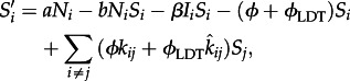
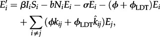
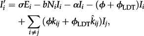
The equations for our ODE model are

2.1

2.2

2.3

2.4

2.5

where i and j are a spatial indices, and S_i, E_i and I_i are the number of susceptible, exposed and infected individuals at location i, respectively. The total population size in location i is N_i.

In the absence of infection, population growth is logistic with an intrinsic rate of increase given by a, and a density-dependent mortality rate, b. This results in a stable disease-free equilibrium at () = (a/b, 0, 0) in all locations i. Our estimate for the intrinsic rate of increase, a, is 3.67 × 10⁻³ day⁻¹, and is based on a mean birth rate of 1.33 kits per year [37–39]. Our estimate for the density-dependent death rate (b = 2.29375 × 10⁻⁷ day⁻¹) yields 16 000 raccoons per county, equivalent to a density of 10 raccoons km⁻² [40,41]. Our estimated values for these and all other model parameters are summarized in table 1.

Table 1.

Parameter description for ODE model (1–5) and the derived stochastic model and the estimated parameter values used in our results.

parameter	description	value	references
a	per capita birth rate	3.67 × 10−3 day−1	[37–39]
b	non-disease induced, density- dependent death rate	2.293 × 10−7 day−1	[40,41]
β	contact rate	1 × 10−4 (animal days)−1	[34,42]
1/σ	latency period	50 days	[43–45]
1/α	infectious period	14 days	[33,43,46]
ϕi, ψi	local movement rate	6 × 10−6 day−1	[34,47]
ϕLDT	long-distance translocation rate	6 × 10−7 day−1	[35]
kij	fraction of emigrants from j to i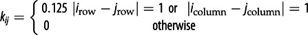

The infection of susceptible individuals occurs at a per capita rate of βI_i where β is the transmission coefficient. Values for β in epidemiological models are often difficult to estimate, because infectious contacts are rarely observed [48]. Given the other model parameters, our estimate for β reproduces the observed 48-month cycle in infectious raccoons [42], and observed net reproductive rate, R₀, for raccoon rabies of approximately 1.2 [34]. The transmission coefficient β must also be scaled to match the spatial resolution of the model since the spread of infection between individuals in our model is a density-dependent process. In estimating values for the transmission rate and emigration rates, we applied a heuristic algorithm that evaluated β in increments of 10⁻⁴, while holding other model parameters fixed to find a value that minimized the absolute difference between the value of a statistic for the model and observed data.

Following infection, there is a latency period during which the virus spreads within a host from the point of infection, through peripheral nerve tissue and into the central nervous system [33]. This is included in the model by the term σE_i in equations (2.3) and (2.4), where 1/σ is the expected length of the latency period. The length of the latency period in raccoons is highly variable and ranges from 18 to 107 days with a mean of approximately 1/σ = 50 days [43–45]. The invasion of the central nervous system is rapidly followed by the migration of virus into the salivary glands and the shedding of virus in the saliva. At this point hosts are infectious, and this phase corresponds with the onset of the end-stage symptoms typical of rabies (e.g. hyper-aggression, hydrophobia, foaming saliva) [33]. Death follows quickly after the onset of symptoms and is included in the model through the term αI_i, where 1/α is the life expectancy of an infectious raccoon. The length of this period is extremely short, on the order of 14 days [33].

Our model includes both local dispersal and LTD of raccoons. Local dispersal is the movement of raccoons over the landscape in search of food, mates and shelter. Local dispersal of hosts is included in the model equations, where ϕ is the per capita dispersal rate. The rate of arrival from surrounding locations, j, into location i is governed by ϕk_ij, where k_ij is the fraction of dispersers from j that arrive in location i. The k_ijs satisfy the condition that all emigrants from location j arrive in one of the surrounding areas (i.e. Σk_ij = 1).

We use coefficients, k_ij, that restrict raccoon dispersal to the eight adjoining locations (a Moore neighbourhood) based on the spatial scale of the model (40 × 40 km²) and the relatively short dispersal distance reported for raccoons (0.5 to 10 km year⁻¹) [40,49]. Our earlier analysis of raccoon rabies data estimated the speed of rabies spread to be between 34.6 and 42.2 km year⁻¹ [34,47]. The emigration rate, ϕ = 6 × 10⁻⁶ day⁻¹, results in rabies spread of 38.4 km year⁻¹. Detailed analysis of the raccoon rabies data for Connecticut indicates the rate of LTD is an order of magnitude smaller than the rate of local dispersal [35]. On this basis we have set the maximum rate of LTD at ϕ_LDT = 6 × 10⁻⁷ day⁻¹.

Our model landscape is 600 × 1400 km divided into 525 (15 × 35) and 40 × 40 km patches. The total model area (840 000 km²) and the patch size (1600 km²) approximate the area affected by the mid-Atlantic raccoon rabies epidemic [50] and the average size of counties in the eastern USA (see the electronic supplementary material, figure S1). Patches within our landscape are connected by the local movement of raccoons between adjoining locales, and by LDT that allows movement across the entire landscape.

(b). Stochastic model

Equations (2.1)–(2.5) are used to form a stochastic model following the method described by Gillespie [36]. Gillespie's method involves reconstituting the continuous dynamical model into a sequence of discrete events that represent the individual processes embodied within a system of differential equations. Gillespie's method provides a formal framework for determining the mean time-step between events, r, as well as the probability distribution of events that may occur at each step. Our equations include the effects of 13 distinct types of events: births (aN_i), density-dependent deaths arising from non-disease related processes (bN_iS_i, bN_iE_i, bN_iI_i), infection of susceptible individuals (βS_iI_i), the progression of the host from latent incubation of the virus to infectiousness (σE_i), the death of infectious individuals of rabies (αI_i) and the local and LDT of individuals in each disease class (ϕS_i, ϕE_i,ϕI_i, ϕ_LDTS_i, ϕ_LDTE_i,ϕ_LDTI_i).

The sum of all the terms on the right-hand side of equations (2.1)–(2.3) is the total rate (r) at which events of all types occur within the population. That is, the total rate at which events occur is

2.5

The inverse, 1/r, is the expected time between events, and is used to determine how much time elapses between events. The probability that a particular event occurs is given by the current rate for that event normalized by the total rate. For example, the probability that an infection will occur at the next event time is βS_iI_i/r. The individual probabilities are combined to create a probability mass function of events (summarized in the electronic supplementary material, table S1) that determines the probability distribution of events.

The model dynamics are created by repeatedly computing the time to the next event, updating the model clock to the new time and choosing the type of the next event based on the probability mass function. At each step in the model, the expected time, 1/r, and the new probability mass function are recomputed from current values for the rates of each event type. The time to the next event is drawn at random from an exponential distribution with mean 1/r. Time is updated to the next event time and the type of event that occurs is determined from the probability mass function. The process repeats until the desired simulation length is reached.

(c). Infection tree and molecular evolution

The link between the dynamics of infection spread and the viral phylogeny is the bifurcating tree of infection events that emerges as the pathogen spreads from host to host (see the electronic supplementary material, figure S2a). The second component of our model tracks the entire bifurcating tree of infections created as rabies infection is spread from one host to another. The infection of one host by another is represented by a fork, or node, in the tree. The two branches that extend from the node represent the source of infection and the newly infected individual. The branch that enters the node represents the originally infected individual. The length of each branch is measured in units of time and marks the interval between infection events. The root of the tree is the index case for the epidemic and the branch tips represent living hosts infected with rabies. The entire tree is a record of the spread of the virus between individual members of the population. It can be used to determine the chain of infectious antecedents that connect a particular individual to the index case or the infectious descendents that follow from a single infected individual.

As the disease spreads, each fork in the infection tree is a potential point of molecular diversification for the virus. The third component of our model simulates the molecular evolution of the virus along the branches and nodes of the infection tree. Once a new host has been infected, the processes of mutation and fixation occur independently in the two viral populations, and the substitutions that characterize each viral population accumulate independently (governed by a common evolutionary model and rate). The accumulated differences in the sequence are the basis for the molecular diversification of the viral phylogeny. Further, because of the rapid evolutionary rate of RNA viruses, the structure of viral phylogeny closely follows the structure of the infection tree (see the electronic supplementary material, figure S2).

(d). Skyline plot analysis

We measure the overall growth of an epidemic based on the rate of increase in the effective number of infections (N_eτ) revealed through a skyline plot analysis [20]. For each replicate run, we extracted the infection tree that connected 100 infected raccoons selected at random, and simulated the molecular evolution of the virus along the nodes and branches of the infection tree to produce a viral phylogeny. We then computed a generalized skyline plot for each viral phylogeny using the R package ape [51] to estimate the change over time in the effective number of infections (N_eτ). Next, we used maximum-likelihood to fit both a time-squared (N_eτ = π(vt + b)²) and exponential (N_eτ = Be^λt) model of growth to the log-transformed time-series of N_eτ values produced by the skyline analysis. We used ΔAIC to determine which of the two growth models was a better fit.

(e). Spatial analysis

For each rate of LDT, we correlated the pairwise geographical and genetic distances to assess the magnitude of IBD. For each correlation we use the slope (m_IBD) and the correlation coefficient () of IBD to measure the strength of the relationship between geographical and genetic distance. The slope (m_IBD) of the correlation indicates the rate at which the genetic distance between samples increases with increasing geographical distance. The IBD correlation coefficient () is a measure of the amount of variation accounted for by a linear relationship. The slope and correlation coefficient together reflect the strength of the correlation and the degree of IBD.

The spatial spread of infection causes viral genotypes to occur in clusters that partition the landscape into patches (see the electronic supplementary material, figure S3) [34,52]. We computed the total area and the area of overlap of the geographical ranges encompassed by clusters of related viral genotypes. The area and overlap of genetic clusters explicitly includes the hierarchical details of the viral phylogeny. A single convex polygon (i.e. one with no concave features) that just encompasses a set of related viral genotypes can be used to define the area occupied by a viral lineage. The area of such a polygon is expected to increase as the rate of LDT is increased because related viral genotypes are more likely to be separated at higher rates of dispersal. The aggregation of genetic lineages into groups contains an element of arbitrariness. We address this issue by defining the endemic phase groups in terms of transition time t_T, at which the epidemiological dynamics shift from epidemic to endemic. Specifically, we are interested in those groups of viruses where all isolates share a common ancestor ‘a’ that is more recent than t_T and that maximize the number of isolates within each group.

(f). Sensitivity analysis

We performed a sensitivity analysis of our model to see if our results were robust to changes in the model parameters. We performed an additional 12 runs in which we either increased or decreased by 10 per cent the value of each of the six model parameters (a, b, β, σ, α, ϕ). We also considered an increased spatial domain for our model (50 × 30 cells) to explore the possibility that our results were scale-dependent or influenced by close proximity of the landscape boundaries along the long axis of the model domain.

In contrast to our model, real-world landscapes are spatially heterogeneous which can introduce noise to biological processes that makes detecting patterns difficult. For example, random variations in habitat quality may result in spatial variation in the demography of the host population and may alter the pattern and tempo of an epidemic. We addressed the question whether such spatial heterogeneity could obscure the phylogenetic signatures associated with different rates of LDT by making the local carrying capacity of each cell and the rate of movement between cells spatially random variables.

To vary carrying capacity, we assigned a random value to the per capita birth rate, a, to each location in our simulated landscape. Random values were drawn from a lognormal distribution with a mean equal to the baseline birth rate (table 1). The variance for the distribution was chosen to place half of distribution area between ±10% of the mean value and half outside these limits (see the electronic supplementary material, figure S4). This resulted in the carrying capacity ranging between 7.5 and 13.3 raccoons km⁻² at 95 per cent of locations. Spatial variation in the dispersal rates was created using the same method of assigning a random deviate to each location from a lognormal distribution centred at the mean local dispersal rate (ϕ = 6 × 10⁻¹ day⁻¹).

For each replicate run of the model we created a new random landscape that was held constant over the course of each replicate. We considered scenarios that included stochastic variation in the carrying capacity only, variation in the dispersal rate only and a scenario in which spatial variation in both demographic parameters was combined.

3. Results

We find that there are unique signatures embedded within the structure of the viral phylogeny produced by different rates of LDT. Skyline plots reveal the effects of LDT as changes in the growth rate of the effective number of infections (N_eτ; figure 1a). As we hypothesized, there are discernible and diagnostic differences in the pattern of growth characteristics of the epidemic with and without LDT. Our results, based on the sign of ΔAIC and summarized in table 2, support our hypothesis that epidemics characterized by local dispersal (ϕ_LDT = 0) should follow a time-squared pattern of growth while exponential growth will arise when spatial spread includes LDT. In 72.5 per cent of epidemics without LDT the time-squared model is a better fit to the skyline data (N_eτ ). On the other hand, exponential growth is a better fit in 80–94.7% of epidemics when LDT is included as a mode of host dispersal (ϕ_LDT ≠ 0). Increasing rates of LDT also produce differences in the phylogenetic structures that can be revealed as increasing rates of growth in the skyline analysis. Higher rates of LDT result in faster epidemic growth rates with a linear relationship between the rate of exponential growth and the non-zero rate of LDT (λ = 4.02 × 10³ϕ_LDT + 2.1 × 10⁻⁴, R² = 0.68, p < 0.001) (figure 1b).

Figure 1.

(a) Skyline plots of the effective number of infections for six rates of LDT (red, ϕ_LDT = 0; yellow, ϕ_LDT = 3.73 × 10⁻⁸; green, ϕ_LDT = 7.5 × 10⁻⁸; cyan, ϕ_LDT = 1.5 × 10⁻⁷; blue, ϕ_LDT = 3 × 10⁻⁷; violet, ϕ_LDT = 6 × 10⁻⁷). Irregular curves show the mean of 40 replicate skyline plots for each rate of LDT. Smooth lines are the mean of 40 regressions fitted to 40 replicate skyline plots for each rate of LDT. The segmented regressions were fitted to the log-transformed effective number of infections (N_eτ). For ϕ_LDT ≠ 0 we fit an exponential model to each of the 40 replicate skyline plots (e.g. N_eτ = Ce^λt), whereas for ϕ_LDT = 0, we fitted a time-squared model (N_eτ = π(vt + b)²). In each case, the mean regression is based on the mean of the parameters (e.g. ). The regressions are based on N_eτ during the spatial spread of infection. The beginning and ending times for spatial spread are parameters of the regression model and are estimated as part of the fit for each replicate skyline plot [53] (see the electronic supplementary material). (b) The change in the exponential rate of growth of the effective number of infections (N_eτ) versus the rate of LDT (ϕ_LDT). Each point is the mean growth rate (λ) and the bars are the standard error of the mean. The red line is the linear regression fitted to the 240 growth rates computed from the model results (40 runs for each of five rates of LDT).

Table 2.

Percentage of replicates in which the epidemic growth is better described by either a time-squared or exponential model of growth. ΔAIC values comparing maximum-likelihood fits of an exponential model of epidemic growth and a time-squared model of growth. For each comparison we computed the difference between the AIC for the exponential model and the time-squared model (ΔAIC = AIC_exponential − AIC_time-squared). (Smaller AIC values are associated with a better fit.) Positive ΔAIC values indicate a smaller AIC value for the time-squared and a better fit by the time-squared model of growth, while negative ΔAIC indicate a better fit by the exponential model of growth. (Absolute number of replicates better described by each growth model are shown parenthetically.)

LDT rate (ϕLDT)	N replicatesa	time-squared growth	exponential growth
0	40	72.5% (29)	27.5% (11)
3.75 × 10−8	40	20% (8)	80% (32)
7.5 × 10−8	38	5.3% (2)	94.7% (36)
1.5 × 10−7	37	18.9% (7)	81.1% (30)
3.0 × 10−7	36	8.3% (3)	91.7% (33)
6.0 × 10−7	38	10.5% (4)	89.5% (34)

^aThe number of replicate runs varies because the model is stochastic, and in some runs the epidemic goes extinct before reaching the end of the 20 year simulation.

Variation in the value of the model parameters produced results that were similar to those observed using the baseline parameter values. The relationship between the non-zero rates of LDT and the exponential growth rate of the epidemic (λ) remained positive and linear, with the slope of the relationship ranging between 1.9 × 10³ and 7.5 × 10³ (see the electronic supplementary material, figure S5). The time-squared function continued to be the best fit to the growth of N_eτ when ϕ_LDT = 0, and the exponential function continued to be the best fit to growth when ϕ_LDT ≠ 0 (see the electronic supplementary material, table S2). Our results on a larger landscape were qualitatively similar to those produced on the original landscape (see the electronic supplementary material, table S2). The results of our sensitivity analysis are given in the electronic supplement.

Our results were also robust to landscape heterogeneity in the host carrying capacity and local dispersal rates. The time-squared model of growth was still a better fit when there was only local dispersal (ϕ_LDT = 0), and the exponential growth model was the better fit in the presence of LDT (see the electronic supplementary material, table S2). In addition, the positive relationship between the rate of LDT and the rate of exponential growth was nearly identical to the relationship obtained from the model without spatial heterogeneity.

We used our model to directly compare the true demographic process of disease spread to the estimate derived from the skyline plots. Such a comparison provides insight into the degree of correlation between skyline reconstruction and the population dynamics when there are multiple complicating factors such as spatial structure and demographic stochasticity. We found the effective number of infections (N_eτ) did not reflect the total number of infected hosts (I_total) when the two datasets were compared directly. Linear regressions of number of infected hosts on N_eτ had low coefficients of determination (R²) and slopes that were not significantly different from zero. However, the lack of correspondence was in large part due to demographic stochasticity to which the skyline plots are not sensitive. On the other hand, we found a strong correspondence when we used the rate of exponential growth to compare the demographic data to the skyline reconstructions. A linear regression of the rates of exponential growth from both sources indicates a strong linear relationship between the two (figure 2).

Figure 2.

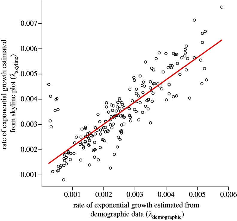
Linear relationship between the exponential growth rate estimated from the viral phylogeny (λ_skyline) and the rate estimated from the demographic record of the epidemic (λ_demographic). Best-fit linear regression is shown in red (λ_skyline = 0.88 × λ_demograph + 0.001, R² = 0.71). Each point represents the rate of exponential growth estimated from the demographic data and the skyline plot from a single replicate run of our model. The plot shows results for all replicates and all positive rates of LDT (ϕ_LDT ≠ 0). The exponential growth rates, λ_skyline, referred to here are the same as the growth rates, λ, that appear on the ordinate of figure 1b, with the subscript added in this figure to make clear distinction with the growth rate estimated from the demographic data (λ_demographic).

We also found that the demographic data was not as reliable a source as the skyline plots for detecting the differences between time-squared and exponential growth. For each replicate run, we computed the daily total number of infected hosts, I_total, from the spatial dynamics. We then fitted models that assumed either time-squared or exponential growth during the period of spatial spread to the time-series of I_total. Maximum likelihood was used to estimate values for the growth model parameters and AIC was used to compare the relative fit of each model with the demographic data. Unlike our results for the skyline plot (table 2), the time-squared growth model was not the better fit to the demographic data when ϕ_LDT = 0 and instead the exponential model was a better fit to I_total both with and without LDT (see the electronic supplementary material, table S4). The difficulty in detecting time-squared growth arises because the demographic data is noisy as a result of demographic stochasticity. This tends to mask differences between time-squared and exponential growth.

We apply our model to explore the mode of epidemic growth exhibited by the mid-Atlantic raccoon rabies epidemic reported by Biek et al. [34]. Based on their analysis, Biek et al. [34] divided the raccoon rabies epidemic into three phases of epidemic expansion corresponding to different physical features of the landscape over which the epidemic spread. We have re-examined these three phases and performed a maximum-likelihood fit of a time-squared versus exponential model to the growth in each phase (phase 1: 1975 through 1982, figure 3a; phase 2: 1986 through 1989, figure 3b; phase 3: 1989 through 1992, figure 3c). As in the analysis of our model results, we use ΔAIC to summarize the relative fit of the two modes of epidemic growth. The procedure we followed to perform the maximum-likelihood fit are described in the electronic supplementary material.

Figure 3.

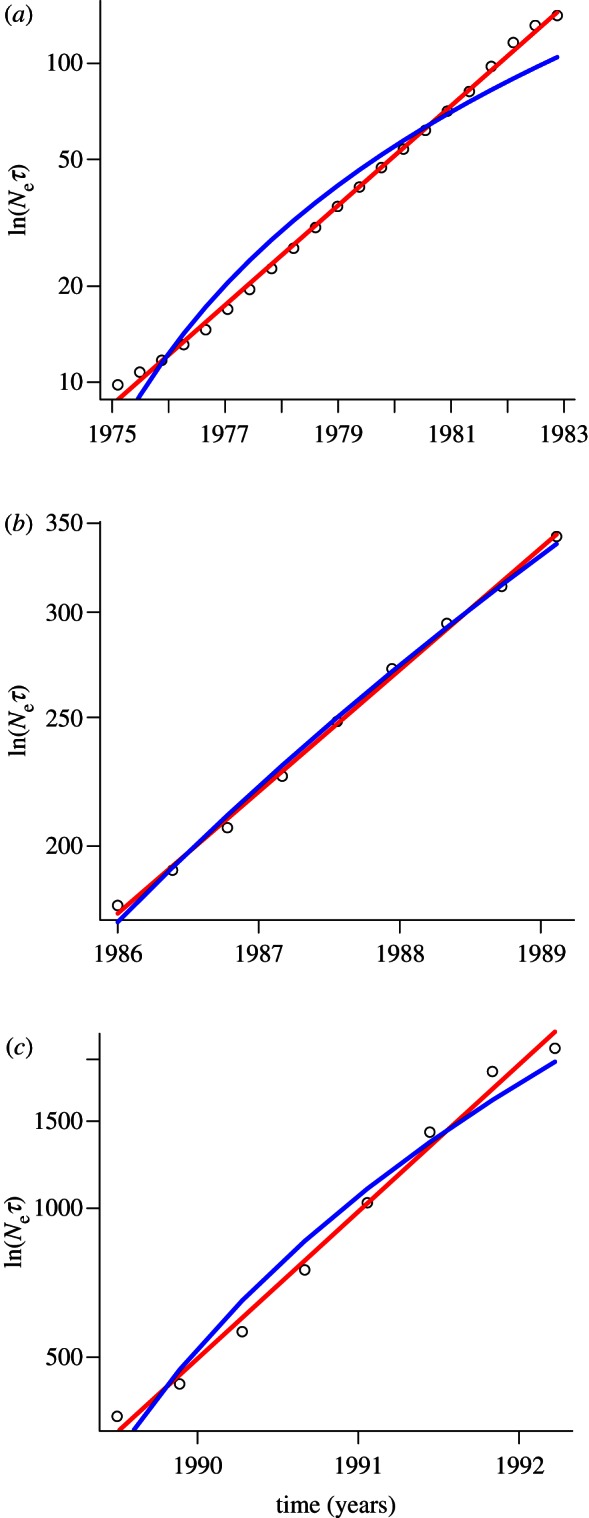
Growth in the effective number of infections (N_eτ) during the three phases of the mid-Atlantic raccoon rabies epidemic [34]. In each panel the circles show the growth in N_eτ obtained from a Bayesian skyline plot analysis of 44 rabies sequences [34], the red line shows the fit of an exponential growth model and the blue line shows a time-squared model of growth. For each phase of the epidemic the exponential model of growth is a better fit ((a) ΔAIC = −65.2; (b) ΔAIC = −6.6; (c) ΔAIC = −9.6), suggesting that long-distance translocation facilitated the spread of rabies in the mid-Atlantic epidemic.

We find that in each phase, the exponential model was a better fit to the Bayesian skyline data than the time-squared model (phase 1: ΔAIC = −65.2; phase 2: ΔAIC = −6.6; phase 3: ΔAIC = −9.6). Based on the classification derived from our model, these results suggest that LDT of infected hosts was not only occurring, but also had a pronounced effect during the mid-Atlantic spread of raccoon rabies. While we are not claiming this as definitive proof of a role of LDT, the exponential growth observed in the phylogenetic data is consistent with an analysis of the demographic data which found that LDT occurred frequently during the spread of raccoon rabies in Connecticut [35].

We are also able to use our model results to quantify the relationship between the spatial distribution of viral lineage and rate of LDT. We find that the degree of IBD and the rate of LDT follow a power law ( () (figure 4a). These results indicate that the strength of IBD will vanish as the rate of LDT increases. This is to be expected since faster rates of LDT will tend to homogenize the landscape, causing all viral genotypes to become evenly distributed in space. More specifically, the small value for the scaling factors linking ϕ_LDT and m_IBD suggest a persistent signature of IBD over a wide range of LDT rates. We find that the area encompassed by genetic groups and the area of overlap between groups increase as the rate of LDT increases (figure 4b). These changes reflect changes in the local spatial structure of the landscape under different rates of LDT. However, as the rate of LDT increases beyond a threshold, the area of groups and overlap reach an upper limit. The upper limit is a consequence of the finite landscape over which an infectious disease could spread.

Figure 4.

Indicators of spatial structure created by different rates of LDT. (a) Change in the strength of IBD at different rates of LDT. When there is long-distance dispersal between locations (ϕ_LDT ≠ 0) the slope (red) and correlation coefficient (blue) both decrease directly as the log of the LDT rate increases. Regression lines were fitted to the data from individual replicates (m_IBD =−0.298 ln(ϕ_LDT) + 0.57, p = 0.012; R_IBD² =−0.03 ln(ϕ_LDT) – 0.232, p = 2.55×10⁻¹⁰). (b) The area of genetic groups (red) and the area of overlap between groups (blue) at six rates of LDT. Points are means and the bars show the standard error of the mean for the replicates at each rate of LDT.

4. Discussion

Our results suggest that differences in fundamental ecological processes, represented in our analysis by differences in the magnitude of LTD, may result in detectable differences in the topology and geographical pattern of pathogen phylogenies. These differences in genetic effects leave a persisting ‘signature’ indicative of specific ecological processes. Even when samples collected from an epidemic reflect many local processes interacting over space, different rates of LDT leave a detectable signature within a viral phylogeny.

Our model includes the demographic stochasticity of the host's birth/death process as well as the disease cycle of rabies from transmission, to incubation, infectiousness and finally death. We have also considered the effects of spatial heterogeneity in the demography of the host species. Despite the considerable noise these processes are expected to add, we are able to reveal several differences in the phylogeny of the virus produced by LDT. Using skyline plots to examine the sequence of coalescent events in the viral phylogeny, we can compare the rate of growth of the epidemic for different movement scenarios. In accordance with our expectations, we find that epidemic growth without LDT follows a time-squared function, whereas growth with LDT is exponential. Further, we find an increasing linear relationship between the rate of exponential growth and the log-transformed rate of LDT.

Our comparison of the skyline plots to the epidemic dynamics indicates that the skyline analysis can provide a reliable estimate of the true demographic changes in the host population. We found that the rate of exponential growth estimate from N_eτ was in close agreement with the rate estimate taken directly from the demographic data (figure 2).

Our results also point to the value of combining phylogenetic analysis with analysis of demographic data collected from an epidemic. We found that the mode of epidemic growth may be easier to detect from the signatures embedded in the viral phylogeny than from the analysis of the demographic data. Time-squared and exponential growth were distinguishable from the pattern of the viral phylogeny (table 1), but this was not the case using only demographic data (see the electronic supplementary material, table S4). Demographic stochasticity in the dynamics of an epidemic introduce noise into the demographic data which may tend to obscure differences between ecological processes such as the model of dispersal. On the other hand, while the rate of rabies virus evolution is fast, it is still not capable of tracking day-to-day changes in the size of an epidemic, and so may be providing a smoother picture of epidemic growth.

In an earlier analysis, solely based on ecological data, we established the importance of LDT during the spread of raccoon rabies in Connecticut over a five-year period of expansion [35]. Mathematical models simulating the dynamics of spread that included LDT as a distinct process result in a better agreement with the observed pattern of spread relative to models that did not include LDT. This earlier analysis used models and data calibrated at the spatial scale of townships, with a mean area of 85 km². Our current analysis, however, suggests that the effects of LDT are preserved across spatial scales. The spatial resolution of our analysis of the entire eastern seaboard epidemic is at the level of counties, with a mean area of 1600 km². The combined analysis reveals a process of expansion characterized by foci of secondary infection acting in advance of the encroaching epidemic wave at both local and regional spatial scales.

Our model results are also consistent with results suggesting that there may have been considerable heterogeneity in the rate of rabies spread in the eastern USA. Using a model that allowed for overdispersed variation in the rate of spread along different branches in the phylogeny (a relaxed random walk), Lemey et al. [54] document a better fit to the genetic data than a time-homogeneous Brownian diffusion model. As an important distinction, the approach by Lemey et al. is focused on revealing and quantifying heterogeneity in the spatial diffusion process from geo-referenced samples without being tied to any particular ecological mechanism. Variation in branch-specific diffusion rates in their case may thus occur for a variety of reasons, including variation in the rate of local spread, the existence of dispersal barriers as well as some contribution of long-distance dispersal. Here, we suggest a complementary approach in which genetic data is analysed with a model that makes explicit the contribution of different modes of dispersal and can be used to make predictions about spatial patterns of growth.

Our analysis based on skyline plots does not include spatial location information from our spatially explicit model. However, our results suggest that phylogenetic patterns associated with spatial processes can be detected even when reliable spatial data are not available. Collection of spatial data that span the period of an epidemic has been an important asset in reconstructing the geographical spread of several infectious diseases including foot and mouth disease [55], and rabies [34,50,54]. However, the collection of accurate and complete public health data is a significant challenge in many parts of the world [56–59]. Our results suggest that analysis of viral sequence data may be useful in overcoming some of these data deficiencies.

Our results are based on viral sequences collected 20 years after the start of the epidemic, when the disease is well into its endemic phase. We chose this retrospective sampling regime because long delays between when an epidemic starts and when it is first sampled are common in infectious disease studies. Wildlife diseases are notoriously difficult to detect because of insufficient surveillance [60]. Even in human populations, epidemics can go unnoticed for prolonged periods of time as highlighted by the discovery of HIV in the early 1980s nearly 30 years after the virus’ suspected emergence in Africa [61,62]. The late sampling date allows for prolonged action of stochastic processes, such as genetic drift and small numbers of infected hosts, which tend to obscure the effect ecological processes have on the viral phylogeny. Despite this, we find that differences in the mode and tempo of dispersal can be recovered from the viral phylogeny (figures 1,3 and 4) decades later. We expect alternative sampling procedures that include collection of some or all samples at times closer to the start of an epidemic to provide better estimates of past ecological processes.

Our results also indicate that at the spatial scale of US counties used in our model, the ability to detect the effects of LDT are limited if sampling were to occur immediately after the start of an epidemic. The skyline plots for different rates of LDT in figure 1a overlap and are essentially indistinguishable in the period immediately following the epidemic. As a result, it would be impossible to detect differences associated with different rates of LDT. This outcome is expected because early in the epidemic there will have been few or no opportunities for LTD events larger than a single county to occur. In such fortunate circumstances where an epidemic is identified before it has a chance to spread, direct monitoring of the epidemic would be a more efficacious approach to studying the disease dynamics. In addition, highly accurate geo-referenced genotype data may allow an earlier assessment of the role of LDT than we observe in our model. However, the chance to observe an epidemic from its very beginning is likely to be the exception. For many epidemics, in both human and wildlife populations, techniques and theory can help reveal unobserved epidemic dynamics.

As long as mutational events occur on similar time-scales as the generation time and the time-scales of spatial movement of the pathogen, this should result in the emergence of phylogeographic structure that can yield insights into the ecological processes that shape the spread of disease, here specifically dispersal. Systems this may apply to are other viruses in terrestrial wildlife hosts, such as hanta- or arenaviruses (potentially long infectious periods offset by limited dispersal ability in the host) or canine distemper, as well as certain plant viruses.

References

- 1.Hutchinson GE. 1965. The ecological theater and the evolutionary play. New Haven, CT: Yale University Press [Google Scholar]
- 2.van Baalen M, Sabelis MW. 1995. The scope for virulence management: a comment on Ewalds view on the evolution of virulence. Trends Microbiol. 3, 414–416 (doi:10.1016/S0966-842X(00)88991-X) [DOI] [PubMed] [Google Scholar]
- 3.Lively CM. 2010. An epidemiological model of host-parasite coevolution and sex. J. Evol. Biol. 23, 1490–1497 (doi:10.1111/j.1420-9101.2010.02017.x) [DOI] [PubMed] [Google Scholar]
- 4.McPeek MA, Holt RD. 1992. The evolution of dispersal in spatially and temporally varying environments. Am. Nat. 140, 1010–1027 (doi:10.1086/285453) [Google Scholar]
- 5.Otto SP, Whitlock MC. 1997. The probability of fixation in populations of changing size. Genetics 146, 723–733 [DOI] [PMC free article] [PubMed] [Google Scholar]
- 6.Gienapp P, Teplitsky C, Alho JS, Mills JA, Merila J. 2008. Climate change and evolution: disentangling environmental and genetic responses. Mol. Ecol. 17, 167–178 (doi:10.1111/j.1365-294X.2007.03413.x) [DOI] [PubMed] [Google Scholar]
- 7.Franks SJ, Sim S, Weis AE. 2007. Rapid evolution of flowering time by an annual plant in response to a climate fluctuation. Proc. Natl Acad. Sci. USA 104, 1278–1282 (doi:10.1073/pnas.0608379104) [DOI] [PMC free article] [PubMed] [Google Scholar]
- 8.Solano P, et al. 2009. The population structure of Glossina palpalis gambiensis from island and continental locations in coastal Guinea. PLoS Negl. Trop. Dis. 3, 1–9 (doi:10.1371/journal.pntd.0000392) [DOI] [PMC free article] [PubMed] [Google Scholar]
- 9.Bradshaw WE, Holzapfel CM. 2001. Genetic shift in photoperiodic response correlated with global warming. Proc. Natl Acad. Sci. USA 98, 14 509–14 511 (doi:10.1073/pnas.241391498) [DOI] [PMC free article] [PubMed] [Google Scholar]
- 10.Rambaut A, Posada D, Crandall KA, Holmes EC. 2004. The causes and consequences of HIV evolution. Nat. Rev. Genet. 5, 52–61 (doi:10.1038/nrg1246) [DOI] [PubMed] [Google Scholar]
- 11.Worobey M, Bjork A, Wertheim JO. 2007. Point, Counterpoint: the evolution of pathogenic viruses and their human hosts. Annu. Rev. Ecol. Syst. 38, 515–540 (doi:10.1146/annurev.ecolsys.38.091206.095722) [Google Scholar]
- 12.Holmes EC, Duffy S, Shackelton LA. 2008. Rates of evolutionary change in viruses: patterns and determinants. Nat. Rev. Genet. 9, 267–276 (doi:10.1038/nrg2323) [DOI] [PubMed] [Google Scholar]
- 13.Gojobori T, Moriyama EN, Kimura M. 1990. Molecular clock of viral evolution, and the neutral theory. Proc. Natl Acad. Sci. USA 87, 10 015–10 018 (doi:10.1073/pnas.87.24.10015) [DOI] [PMC free article] [PubMed] [Google Scholar]
- 14.Li WH, Tanimura M, Sharp PM. 1988. Rates and dates of divergence between AIDS virus nucleotide-sequences. Mol. Biol. Evol. 5, 313–330 [DOI] [PubMed] [Google Scholar]
- 15.Tanaka Y, Hanada K, Mizokami M, Yeo AET, Shih JWK, Gojobori T, Alter HJ. 2002. A comparison of the molecular clock of hepatitis C virus in the United States and Japan predicts that hepatocellular carcinoma incidence in the United States will increase over the next two decades. Proc. Natl Acad. Sci. USA 99, 15 584–15 589 (doi:10.1073/pnas.242608099) [DOI] [PMC free article] [PubMed] [Google Scholar]
- 16.Fu YX. 1994. A phylogenetic estimator of effective population size or mutation rate. Genetics 136, 685–692 [DOI] [PMC free article] [PubMed] [Google Scholar]
- 17.Nee S, Holmes EC, Rambaut A, Harvey PH. 1995. Inferring population history from molecular phylogenies. Phil. Trans. R. Soc. Lond. B 349, 25–31 (doi:10.1098/rstb.1995.0087) [DOI] [PubMed] [Google Scholar]
- 18.Drummond AJ, Rambaut A, Shapiro B, Pybus OG. 2005. Bayesian coalescent inference of past population dynamics from molecular sequences. Mol. Biol. Evol. 22, 1185–1192 (doi:10.1093/molbev/msi103) [DOI] [PubMed] [Google Scholar]
- 19.Pybus OG, Rambaut A, Harvey PH. 2000. An integrated framework for the inference of viral population history from reconstructed genealogies. Genetics 155, 1429–1437 [DOI] [PMC free article] [PubMed] [Google Scholar]
- 20.Strimmer K, Pybus OG. 2001. Exploring the demographic history of DNA sequences using the generalized skyline plot. Mol. Biol. Evol. 18, 2298–2305 (doi:10.1093/oxfordjournals.molbev.a003776) [DOI] [PubMed] [Google Scholar]
- 21.Holmes EC, Grenfell BT. 2009. Discovering the phylodynamics of RNA viruses. PLoS Comput. Biol. 5 [DOI] [PMC free article] [PubMed] [Google Scholar]
- 22.de Quadros CA, Olive JM, Hersh BS, Strassburg MA, Henderson DA, Brandling-Bennett D, Alleyne GA. 1996. Measles elimination in the Americas. Evolving strategies. JAMA 275, 224–229 (doi:10.1001/jama.1996.03530270064033) [DOI] [PubMed] [Google Scholar]
- 23.Fevre EM, Bronsvoort BMDC, Hamilton KA, Cleaveland S. 2006. Animal movements and the spread of infectious diseases. Trends Microbiol. 14, 125–131 (doi:10.1016/j.tim.2006.01.004) [DOI] [PMC free article] [PubMed] [Google Scholar]
- 24.Centers for Disease Control 2003. Update: severe acute respiratory syndrome—Toronto, Canada, 2003. Morb. Mortal. Wkly. Rep. 52, 547–550 [PubMed] [Google Scholar]
- 25.Rappole JH, Derrickson SR, Hubalek Z. 2000. Migratory birds and spread of West Nile virus in the Western Hemisphere. Emerg. Infect. Dis. 6, 319–328 (doi:10.3201/eid0604.000401) [DOI] [PMC free article] [PubMed] [Google Scholar]
- 26.Snoeck CJ, Adeyanju AT, De Landtsheer S, Ottosson U, Manu S, Hagemeijer W, Mundkur T, Muller CP. 2011. Reassortant low-pathogenic avian influenza H5N2 viruses in African wild birds. J. Gen. Virol. 92, 1172–1183 (doi:10.1099/vir.0.029728-0) [DOI] [PubMed] [Google Scholar]
- 27.Takekawa JY, et al. 2010. Victims and vectors: highly pathogenic avian influenza H5N1 and the ecology of wild birds. Avian Biol. Res. 3, 51–73 (doi:10.3184/175815510X12737339356701) [Google Scholar]
- 28.Hanlon CA, Rupprecht CE. 1998. The reemergence of rabies. In Emerging infections (eds Scheld WM, Armstrong D, Hughes JM.), pp. 59–80 Washington, DC: ASM Press [Google Scholar]
- 29.Bacon PJ. (ed.) 1985. Population dynamics of rabies in wildlife. London, UK: Academic Press [Google Scholar]
- 30.Shigesada N, Kawasaki K. 1997. Biological invasions: theory and practice. Oxford, New York: Oxford University Press [Google Scholar]
- 31.Wright S. 1943. Isolation by distance. Genetics 28, 114–138 [DOI] [PMC free article] [PubMed] [Google Scholar]
- 32.Kermack WO, Mckendrick AG. 1927. Contributions to the mathematical theory of epidemics. Proc. R. Soc. Lond. A 115, 700–721 (doi:10.1098/rspa.1927.0118) [Google Scholar]
- 33.Jackson AC, Wunner W. (ed.) 2007. Rabies. New York: Academic Press [Google Scholar]
- 34.Biek R, Henderson JC, Waller L, Rupprecht CE, Real LA. 2007. A high-resolution genetic signature of demographic and spatial expansion in epizootic rabies virus. Proc. Natl Acad. Sci. USA 104, 7993–7998 (doi:10.1073/pnas.0700741104) [DOI] [PMC free article] [PubMed] [Google Scholar]
- 35.Smith DL, Lucey B, Waller LA, Childs JE, Real LA. 2002. Predicting the spatial dynamics of rabies epidemics on heterogeneous landscapes. Proc. Natl Acad. Sci. USA 99, 3668–3672 (doi:10.1073/pnas.042400799) [DOI] [PMC free article] [PubMed] [Google Scholar]
- 36.Gillespie DT. 1977. Exact stochastic simulation of coupled chemical-reactions. J. Phys. Chem. 81, 2340–2361 (doi:10.1021/j100540a008) [Google Scholar]
- 37.Bissonnette TH, Csech AG. 1938. Sexual photoperiodicity of raccoons on low protein diet and second litters in the same breeding season. J. Mammal. 19, 342–348 (doi:10.2307/1374574) [Google Scholar]
- 38.Johnson AS. 1970. Biology of the raccoon (Procyon lotor varius Nelson and Goldman) in Alabama, Bulletin 402 Auburn, AL: Agriculture Experiment Station, Auburn University [Google Scholar]
- 39.Sheeler L. 2002. Epidemiological model of raccoon rabies in Alabama. Dissertation, Texas Technical University, TX, USA
- 40.Stuewer FW. 1943. Raccoons: their habits and management in michigan. Ecol. Monogr. 13, 203–257 (doi:10.2307/1943528) [Google Scholar]
- 41.Urban D. 1970. Raccoon populations, movement patterns, and predation on a managed waterfowl marsh. J. Wildl. Manage. 34, 372 (doi:10.2307/3799024) [Google Scholar]
- 42.Childs JE, Curns AT, Dey ME, Real LA, Feinstein L, Bjornstad ON, Krebs JW. 2000. Predicting the local dynamics of epizootic rabies among raccoons in the United States. Proc. Natl Acad. Sci. USA 97, 13 666–13 671 (doi:10.1073/pnas.240326697) [DOI] [PMC free article] [PubMed] [Google Scholar]
- 43.Bigler WJ, McLean RG, Trevino HA. 1973. Epizootiologic aspects of raccoon rabies in Florida. Am. J. Epidemiol. 98, 326–335 [DOI] [PubMed] [Google Scholar]
- 44.McLean RG. 1975. Raccoon rabies. In The natural history of rabies (ed. Baer GM.), pp. 53–77 New York, NY: Academic Press [Google Scholar]
- 45.Carey AB, Mclean RG. 1983. The ecology of rabies: evidence of co-adaptation. J. Appl. Ecol. 20, 777–800 (doi:10.2307/2403126) [Google Scholar]
- 46.Niezgoda M, Hanlon CA, Rupprecht CE. 2002. Animal rabies. In Rabies (eds Jackson AC, Wunner W.) pp. 163–218 New York, NY: Academic Press [Google Scholar]
- 47.Smith DL, Waller LA, Russell CA, Childs JE, Real LA. 2005. Assessing the role of long-distance translocation and spatial heterogeneity in the raccoon rabies epidemic in Connecticut. Prev. Vet. Med 71, 225–240 (doi:10.1016/j.prevetmed.2005.07.009) [DOI] [PMC free article] [PubMed] [Google Scholar]
- 48.Real LA, Biek R. 2007. Infectious disease modeling and the dynamics of transmission. In Wildlife and emerging zoonotic diseases: the biology, circumstances and consequences of cross-species transmission (eds Childs JE, Mackenzie JS, Richt JA.). New York, NY: Springer [Google Scholar]
- 49.Gehrt SD. 2003. Raccoons and allies. In Wild mammals of North America (eds Feldhamer GA, Chapman JA, Thompson BC.), 2nd edn Baltimore, MD: Johns Hopkins University Press [Google Scholar]
- 50.Real LA, et al. 2005. Unifying the spatial population dynamics and molecular evolution of epidemic rabies virus. Proc. Natl Acad. Sci. USA 102, 12 107–12 111 (doi:10.1073/pnas.0500057102) [DOI] [PMC free article] [PubMed] [Google Scholar]
- 51.Paradis E, Claude J, Strimmer K. 2004. APE: analyses of phylogenetics and evolution in R language. Bioinformatics 20, 289–290 (doi:10.1093/bioinformatics/btg412) [DOI] [PubMed] [Google Scholar]
- 52.Joy DA, et al. 2003. Early origin and recent expansion of Plasmodium falciparum. Science 300, 318–321 (doi:10.1126/science.1081449) [DOI] [PubMed] [Google Scholar]
- 53.Muggeo VMR. 2003. Estimating regression models with unknown break-points. Stat. Med. 22, 3055–3071 (doi:10.1002/sim.1545) [DOI] [PubMed] [Google Scholar]
- 54.Lemey P, Rambaut A, Welch JJ, Suchard MA. 2010. Phylogeography takes a relaxed random walk in continuous space and time. Mol. Biol. Evol. 27, 1877–1885 (doi:10.1093/molbev/msq067) [DOI] [PMC free article] [PubMed] [Google Scholar]
- 55.Cottam EM, Haydon DT, Paton DJ, Gloster J, Wilesmith JW, Ferris NP, Hutchings GH, King DP. 2006. Molecular epidemiology of the foot-and-mouth disease virus outbreak in the United Kingdom in 2001. J. Virol. 80, 11 274–11 282 (doi:10.1128/JVI.01236-06) [DOI] [PMC free article] [PubMed] [Google Scholar]
- 56.Chan M, Kazatchkine M, Lob-Levyt J, Obaid T, Schweizer J, Sidibe M, Veneman A, Yamada T. 2010. Meeting the demand for results and accountability: a call for action on health data from eight global health agencies. PLoS Med. 7, e1000223 (doi:10.1371/journal.pmed.1000223) [DOI] [PMC free article] [PubMed] [Google Scholar]
- 57.Mate KS, Bennett B, Mphatswe W, Barker P, Rollins N. 2009. Challenges for routine health system data management in a large public programme to prevent mother-to-child HIV transmission in South Africa. PLoS ONE 4, e5483 (doi:10.1371/journal.pone.0005483) [DOI] [PMC free article] [PubMed] [Google Scholar]
- 58.Harpham T. 2009. Urban health in developing countries: what do we know and where do we go? Health Place 15, 107–116 (doi:10.1016/j.healthplace.2008.03.004) [DOI] [PubMed] [Google Scholar]
- 59.Wilkins K, Nsubuga P, Mendlein J, Mercer D, Pappaioanou M. 2008. The Data for Decision Making project: assessment of surveillance systems in developing countries to improve access to public health information. Public Health 122, 914–922 (doi:10.1016/j.puhe.2007.11.002) [DOI] [PubMed] [Google Scholar]
- 60.Hawkins CE, et al. 2006. Emerging disease and population decline of an island endemic, the Tasmanian devil Sarcophilus harrisii. Biol. Conserv. 131, 307–324 (doi:10.1016/j.biocon.2006.04.010) [Google Scholar]
- 61.Yusim K, Peeters M, Pybus OG, Bhattacharya T, Delaporte E, Mulanga C, Muldoon M, Theiler J, Korber B. 2001. Using human immunodeficiency virus type 1 sequences to infer historical features of the acquired immune deficiency syndrome epidemic and human immunodeficiency virus evolution. Phil. Trans. R. Soc. Lond. B 356, 855–866 (doi:10.1098/rstb.2001.0859) [DOI] [PMC free article] [PubMed] [Google Scholar]
- 62.Nzilambi N, et al. 1988. The prevalence of infection with human immunodeficiency virus over a 10-year period in Rural Zaire. N. Engl. J. Med. 318, 276–279 (doi:10.1056/NEJM198802043180503) [DOI] [PubMed] [Google Scholar]