A statistical framework for analyzing hypothesized interactions between cells imaged using multispectral microscopy and multiple immunohistochemical markers

Abstract

Background:

Multispectral microscopy and multiple staining can be used to identify cells with distinct immunohistochemical (IHC) characteristics. We present here a method called hypothesized interaction distribution (HID) analysis for characterizing the statistical distribution of pair-wise spatial relationships between cells with particular IHC characteristics and apply it to clinical data.

Materials and Methods:

We retrospectively analyzed data from a study of 26 follicular lymphoma patients in which sections were stained for CD20 and YY1. HID analysis, using leave-one-out validation, was used to assign patients to one of two groups. We tested the null hypothesis of no difference in Kaplan–Meier survival curves between the groups.

Results:

Shannon entropy of HIDs assigned patients to groups that had significantly different survival curves (median survival was 7.70 versus 110 months, P = 0.00750). Hypothesized interactions between pairs of cells positive for both CD20 and YY1 were associated with poor survival.

Conclusions:

HID analysis provides quantitative inferences about possible interactions between spatially proximal cells with particular IHC characteristics. In follicular lymphoma, HID analysis was able to distinguish between patients with poor versus good survival, and it may have diagnostic and prognostic utility in this and other diseases.

BACKGROUND

Pathologists use microscopic tissue analysis for diagnosis and prognostication of diseases. This is based on visual recognition of particular patterns of distinct cells indicative of specific or general cellular processes. However, it can be difficult or impossible to disambiguate cells in fixed sections using standard illumination methods. In the context of solid tumors, multiple molecular markers—particularly at the protein level using immunohistochemistry—can be imaged using multispectral microscopy.[1] This is an imaging technique in which a section is imaged multiple times, each time illuminated using a distinct and narrow range of wavelengths. The result is a “cube” of optical density data or, equivalently, a spectrum of optical densities at each pixel location. This data can be processed to identify regions or cells that are positive for particular markers (e.g., via thresholding of optical densities and other techniques). However, even with sophisticated analysis and visualization tools, it is difficult for expert clinicians to interpret images acquired using more than a few markers. Furthermore, while it is believed that cells with particular immunohistochemical (IHC) profiles may interact to varying degrees of patient detriment, there are few quantitative methods available for investigating these hypotheses. The present paper presents such a method and demonstrates the application of it to a study of follicular lymphoma (FL).

MATERIALS AND METHODS

Combinatorial Molecular Phenotypes

Given a cube of data from a multiple-stained section imaged using multispectral microscopy, we assumed that it is possible to determine whether each cell in a section is positive (1) or negative (0) for each marker and to obtain cells’ spatial (x, y) co-ordinates. This can be achieved, for example, using commercially available software (e.g., Nuance; PerkinElmer Inc., Waltham, MA, USA). Let 𝕊 denote a set of N markers and the positivity of a cell for stain s ∈ 𝕊 as π_s. We adopt the term “combinatorial molecular phenotype (CMP)” from a previous study[2] that describes the positivity of a cell for all stains in 𝕊 as the binary vector π = (π_s1, …, π_sN), where s_i denotes the i^th stain. For example, a possible CMP for an image stained with three markers may be π = (1, 0, 0). No (x,y) co-ordinates will be recorded for cells that are negative for all markers in 𝕊. Therefore, any of 2^N-1 CMPs may be observed. Each possible CMP can be assigned a unique number according to a suitable binary counting scheme. If the right-most element of a CMP represents the least significant binary digit and the next right-most element represents the next least significant digit and so on, then the vectors (0, 1, 0), (1, 0, 0), and (1, 1, 1) can be numbered 2, 4, and 7, respectively. Because this numbering system begins at 1, it is useful for indexing the matrices we introduce later in this paper.

Combinatorial Molecular Phenotype Approximation

Some software can automatically and accurately segment individual cells using full multispectral data. However, less sophisticated software is limited to segmenting regions from particular sub-bands, giving rise to separate sets of region centroid co-ordinates for each stain, some of which may encompass multiple cells (i.e., inaccurate segmentation). However, it is possible to use the region centroid co-ordinates—obtained for each marker independently—to identify regions that are so sufficiently close that they are likely to correspond to the same cell, and, therefore, to approximate CMPs.

First, regions likely to encompass multiple cells are rejected by discarding those that are larger than the maximum area expected for typical cells. Then, co-ordinates from different markers that are within a “pairing distance,” d_P, are combined into a single co-ordinate to which the appropriate cell CMP is associated. Later in the paper, we have shown how distance d_P may be chosen statistically.

Hypothesized Interaction Distributions

We hypothesized that two cells—sufficiently close together and with identical or different CMPs—may interact to varying degrees of patient benefit or detriment. We call this a “hypothesized interaction.” By extension, we hypothesize that if a particular hypothesized interaction does indeed act in this way, then many such interactions between pairs of cells will have a larger effect on patient outcome.

We formalize the notion of hypothesized interactions and quantify their occurrence by introducing a commutative arrow operator. A particular hypothesized interaction y can be denoted by . The notation can be understood as follows. Consider all possible pairings of cells within a given section, such that no two paired cells are located further than an “interaction distance,” d_I, from one another. The arrow notation specifies that a proportion, p, of all pairings, are between a cell with CMP number i and another with j. This notation is convenient because it can be used to form graphs, which may aid visualization. Later in this paper, we explain how an optimal value of d_I can be chosen statistically.

The proportion p can also be interpreted as a probability. By calculating p for each possible hypothesized interaction, we can define a statistical distribution over them. Let D be a (2^N – 1) × (2^N – 1) symmetric matrix, whose (i, j)^th element is the probability of observing a cell with CMP number i within a distance d_I of a cell with CMP number j. If Y is a random variable that represents a hypothesized interaction, then the statistical distribution of Y can be written as Y ~ D, and we call D a “hypothesized interaction distribution” (HID). Figure 1 shows an example of HIDs and their graphs.

Figure 1.

Example hypothesized interaction distributions and their corresponding graphs

Scalar Summaries of Hypothesized Interaction Distributions

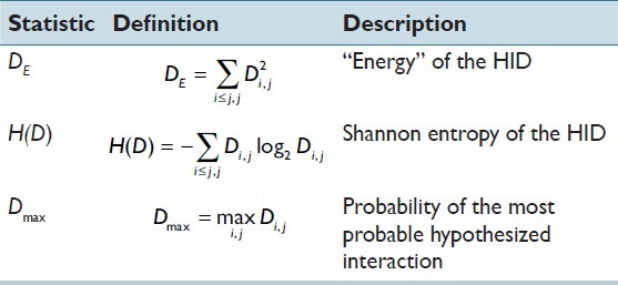
We are interested in testing the hypothesis that cells of particular “types” may interact to varying degrees of patient benefit or detriment. Specifically, we are interested in investigating whether HIDs facilitate the assignment of patients into groups with good versus poor survival. Taking inspiration from grey-level co-occurrence matrix analysis methodology in the texture analysis literature,[3] Table 1 defines three scalar summary statistics that can be used to characterize a HID. Note that the indexing used in the summations accounts for the fact that the upper and lower triangles are symmetric and that only one of these triangles is required to specify the HID (i.e., the elements in one of the triangles sum to unity).

Table 1.

Definitions and descriptions of scalar summary statistics

Distribution “peakiness” is characterized in different ways by D_E and H(D); D_max characterizes the degree to which the most common hypothesized interaction occurs. Shannon entropy, H(D), measures the expected information (in bits) required to transmit a randomly chosen hypothesized interaction, drawn from the distribution D, over an idealized channel. Hypothesized interactions associated with uniform distributions require more information than those from non-uniform distributions.

Assigning Patients to Groups for Survival Analysis

Given a vector of values of a particular summary statistic (e.g., D_max) for n patients, γ = (γ₁, …, γ_n), we can choose an optimal threshold, γ^*_T, on that statistic that best assigns patients to groups on the basis of survival via the optimization

Here, the i^th element of the vector s is the survival time for the i^th patient and the function g_γT returns a vector whose i^th element is the group assignment of the i^th patient resulting from the application of threshold γ_T to the i^th element of the vector γ. The objective function χ² computes the value of the χ² statistic associated with the null hypothesis that the survival curves arising from the group assignments are equal;[4] high values of χ² have corresponding low P values.

Selecting Optimal Pairing and Interaction Distances

The distances d_I and d_P may in principle be selected by the investigator, for example, by drawing upon expert clinical knowledge. However, this approach is subjective and we therefore proposed an objective method. Optimal values (d^*_I,d^*_P) can be chosen statistically via the optimization

This is a modification of equation 1, where γ(d_I, d_P) returns a vector of summary statistics for HIDs computed using distances d_I and d_P.

Application in Follicular Lymphoma

The aims of this experiment were to demonstrate the application of HID analysis to data from multispectral microscopy of multiple-stained tissue sections from a sample of FL patients and to evaluate the method's ability to identify patient groups that differ in survival.

Twenty six archived human lymph nodes from patients (16 male, 10 female, aged 36-77 years, mean 55 years) with a diagnosis of FL were collected at initial diagnosis, prior to the treatment. Written informed consent and local research ethics committee approval were obtained. The material was routinely processed by fixation in formalin and paraffin embedding. Clinical data and up to 14 years of follow-up and survival data were available for each sample (19 dead, 7 alive; median time to death 32 months; range 2-170 months; 171 months follow-up in all patients alive at the end of the study period). Paraffin-embedded sections from these cases were reviewed by two pathologists.

Duplex quantum dot-based immunofluorescence was used to co-localize YY1 with CD20 using a duplex QD-IF protocol.[5] Briefly, tissue sections were subjected to antigen retrieval by microwave heating in Tris-EDTA buffer and incubated with YY1 monoclonal primary antibody (Santa Cruz Biotechnology, Santa Cruz, CA, USA) diluted 1:50 (v/v) in 1:10 (v/v) goat serum overnight at 4°C. Secondary detection was performed using a goat anti-mouse secondary antibody diluted 1:250 (v/v) in 1:10 (v/v) goat serum, followed by 655 nm quantum dot solution (Invitrogen, Carlsbad, CA, USA) (1:50 (v/v) in 1:10 (v/v) goat serum). Sections were washed and incubated with Avidin solution followed by incubation with Biotin solution (Vector Laboratories, Burlingame, CA, USA). An anti-CD20 monoclonal primary antibody (Dako, Glostrup, Denmark) diluted 1:50 (v/v) in 1:10 (v/v) goat serum was then applied for 1 hour at room temperature. Secondary detection was performed using the same protocol as for YY1 with the exception of use of a 605 nm quantum dot solution (Invitrogen) diluted 1:50 (v/v) in 1:10 (v/v) goat serum. Finally, sections were rinsed and mounted in polyvinyl mounting medium with DABCO (Sigma-Aldrich, St. Louis, MO, USA) and sealed with clear nail varnish.

Areas positive for YY1 or CD20 expression were identified by spectral imaging using a LeitzDiaplan fluorescence microscope and a Nuance spectral analyzer. Image cubes were collected and subjected to spectral unmixing using Nuance software version 2.4.2 to generate 2D intensity distributions of YY1 and CD20 positivity; up to five images from different portions of each specimen were taken to help ensure that inferred characteristics were representative. Composite images taken of sections double stained for YY1 and CD20 were unmixed using spectra for 605 nm and 655 nm quantum dots and the resultant 2D intensity maps for each of YY1 and CD20 thresholded to generate biologically relevant positive regions of interest; regions of interest were at least 100 pixels in area. Region centroid co-ordinates, region area, maximum intensity, and average intensity were exported to Excel (Microsoft Corporation, Redmond, WA, USA). All images were captured at a total magnification of ×400 with standardized and uniform image illumination and magnification such that all images captured were directly comparable in terms of intensity and scale.

Very large regions—representing incorrect discrimination between distinct cells—were rejected by discarding regions with area greater than 200 pixels. The topology of the χ² function (equation 2) for each summary statistic was estimated via thin plate spline interpolation[6] of values of χ² function computed on a regular 14 × 24 grid of (d_I, d_P) values. The χ² function is computationally expensive to compute and tends to have multiple maxima. We therefore selected optimal values of d_I and d_P for each summary statistic by inspecting contour plots, favoring maxima near (d_I, d_P) = (0, 0). Approximate CMPs, HIDs, and their summary statistics were constructed for each image. Each patient was represented by the median of each summary statistic, taken over all images acquired for the patient. Finally, Kaplan–Meier survival curves were estimated using leave-one-out validation: at the i^th iteration, the i^th patient was left out of the analysis and an optimal threshold for each summary statistic calculated for the left-in patients (equation 1); this threshold was used to allocate the left-out patient to one of two groups. Software was implemented in R version 2.13.0.[7]

RESULTS

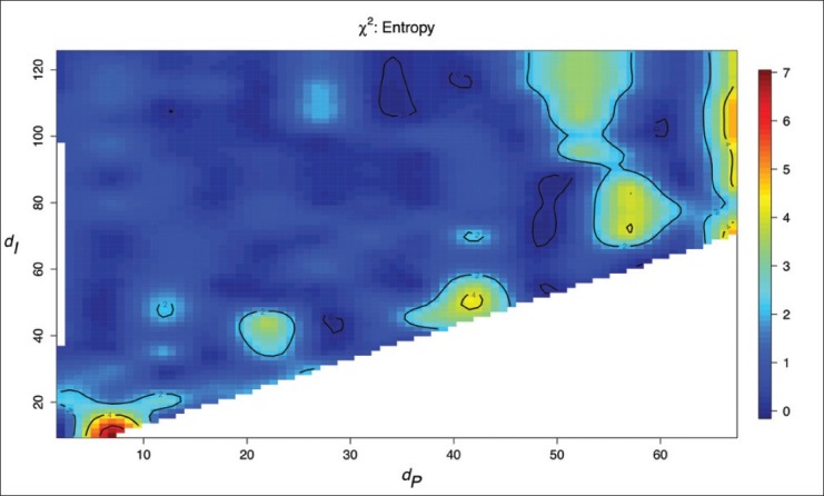
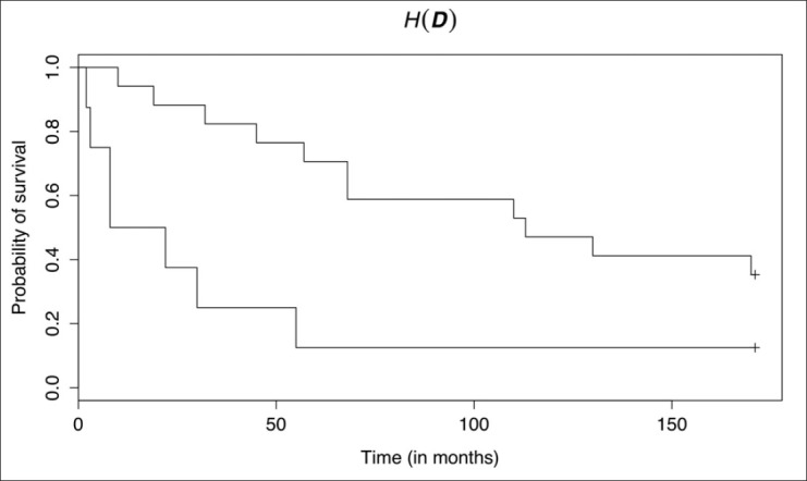
Figure 2 shows the topology of the objective function (equation 2) for H(D) under the constraint that d_P < d_I (as we must pair regions before considering that paired regions may interact). Table 2 shows the results of the leave-one-out survival analyses and the (d^*_I, d^*_P) used. There was a statistically significant difference between the survival curves defined by the summary statistic H(D), but not for D_max and D_E; the P value for H(D) would survive Bonferroni correction for multiple comparisons at the α = 0.05 significance level. Kaplan–Meier survival curves for H(D)—estimated via leave-one-out validation—are shown in Figure 3. Median survival for the two groups is approximately 7.70 and 110 months. Low H(D) (“peaky” distributions) were associated with poor survival and these peaks were often observed for hypothesized interactions between cells that were positive for both YY1 and CD20. Figure 1 shows example HIDs and their graphs for patients with poor (D₁) versus good (D₂) survival.

Figure 2.

Contour plot showing the value of the χ² test statistic as a function of pairing distance d_P and interaction distance d_I for the summary statistic D_max

Table 2.

Leave-one-out analysis results. Optimal values of d_I and d_P, and the resulting P values. The statistically significant (P < 0.05) result for H (D) would survive Bonferroni correction

Figure 3.

Survival curves—estimated using leave-one-out validation—for groups defined by thresholding H(D). The curves are statistically significantly different (P = 0.00750)

CONCLUSIONS

We have developed a statistical framework to represent potential interactions between proximal cells. The method defines a statistical distribution over “hypothesized interactions”—a pairing of cells with particular combinations of IHC characteristics, located within a given distance of one another. These distributions can be represented in matrix and graphical forms. Relatively simple scalar summaries of these distributions can be used to assign patients to groups that may differ in terms of survival, and the distributions themselves can be inspected to identify possible cellular interactions that are associated with short versus long survival.

HID analysis of retrospective data from a study of FL showed that Shannon entropy, H(D), was able to assign patients to groups with significantly different survival curves. Our results suggest that cells that are positive for both YY1 and CD20 may interact to patient detriment. This result is consistent with our understanding of the biology of these cells, but existing analysis tools do not allow testing of this hypothesis.

One limitation of this work is the visual (albeit quantitative and objective) selection of distances d_P and d_I prior to, and outside of, the leave-one-out analysis. Unfortunately, the high computational cost of evaluating the χ² function—and the fact that the function tends to have multiple maxima—made automated selection infeasible within the scope of this work. Future research should address this problem.

In conclusion, HID analysis provides a largely automated quantitative method for making inferences about possible interactions between proximal cells—in terms of their IHC characteristics as measured using multispectral microscopy and multiple IHC markers—with potential value for diagnosis and prognosis.

REFERENCES

- 1.Byers RJ, Hitchman ER. Quantum dots brighten biological imaging. Prog Histochem Cytochem. 2011;45:201–37. doi: 10.1016/j.proghi.2010.11.001. [DOI] [PubMed] [Google Scholar]
- 2.Schubert W. A three-symbol code for organized proteomes based on cyclical imaging of protein locations. Cytometry A. 2007;71:352–60. doi: 10.1002/cyto.a.20281. [DOI] [PubMed] [Google Scholar]
- 3.Haralick RM, Shanmugam K, Dinstein I. Textural features for image classification. IEEE Trans Syst Man Cybern. 1973;3:610–21. [Google Scholar]
- 4.Harrington DP, Fleming TR. A class of rank test procedures for censored survival data. Biometrika. 1982;69:553–66. [Google Scholar]
- 5.Naidoo K, Clay V, Hoyland JA, Swindell R, Linton K, Illidge T, et al. YY1 expression predicts favourable outcome in follicular lymphoma. J Clin Pathol. 2011;64:125–9. doi: 10.1136/jcp.2010.078188. [DOI] [PubMed] [Google Scholar]
- 6.Duchon J. Splines minimizing rotation-invariant semi-norms in Sobolev spaces. In: Schempp W, Zeller K, editors. Constructive Theory of Functions of Several Variables. Vol. 571. Heidelberg: Springer; 1977. pp. 85–100. [Google Scholar]
- 7.R: A Language and Environment for Statistical Computing. Vienna, Austria: R Foundation for Statistical Computing; 2012. [Last accessed on 2013 Jan 21]. R Development Core Team. Available from: http://www.R-project.org . [Google Scholar]