Histological stain evaluation for machine learning applications

Abstract

Aims:

A methodology for quantitative comparison of histological stains based on their classification and clustering performance, which may facilitate the choice of histological stains for automatic pattern and image analysis.

Background:

Machine learning and image analysis are becoming increasingly important in pathology applications for automatic analysis of histological tissue samples. Pathologists rely on multiple, contrasting stains to analyze tissue samples, but histological stains are developed for visual analysis and are not always ideal for automatic analysis.

Materials and Methods:

Thirteen different histological stains were used to stain adjacent prostate tissue sections from radical prostatectomies. We evaluate the stains for both supervised and unsupervised classification of stain/tissue combinations. For supervised classification we measure the error rate of nonlinear support vector machines, and for unsupervised classification we use the Rand index and the F-measure to assess the clustering results of a Gaussian mixture model based on expectation–maximization. Finally, we investigate class separability measures based on scatter criteria.

Results:

A methodology for quantitative evaluation of histological stains in terms of their classification and clustering efficacy that aims at improving segmentation and color decomposition. We demonstrate that for a specific tissue type, certain stains perform consistently better than others according to objective error criteria.

Conclusions:

The choice of histological stain for automatic analysis must be based on its classification and clustering performance, which are indicators of the performance of automatic segmentation of tissue into morphological components, which in turn may be the basis for diagnosis.

INTRODUCTION

Pathologists rely on histological stains to identify morphological changes in tissue that are linked to cancer and other diseases. Different stain combinations target different types of tissue. With the most common stain, hematoxylin/eosin, the hematoxylin stains the cell nuclei blue, and the counter-stain, eosin, stains the cytoplasm pink and stromal components in various grades of red/pink. This and most other stains are developed for visual examination of the tissue under a microscope, and thus they are often not optimal for automated pattern and image analysis. However automated and computer-assisted analysis of histopathology specimens is gaining importance since the introduction of high throughput imaging systems.

As a first step in the automated analysis of tissue samples, morphological components, such as nuclei, stroma, and cytoplasm, often need to be identified and segmented from the surrounding tissue for further analysis. This identification relies on the absorption of histological stains by the tissue components, and therefore the choice of stain has a significant effect on the outcome of the segmentation. Color image analysis for histologically stained tissue is further complicated by both inter- and intra-specimen intensity variations due to variations in the tissue preparation process and overlap in the stain absorption spectra.[1,2]

Quantitative evaluation of the efficacy of a particular stain for automatic color image analysis relies upon the evaluation of the stained tissue in a color space where the distance between two points represents the chromaticity difference between the corresponding colors, reducing the dependence on the intensity variations that may arise from tissue preparation and image acquisition. In such a color space, the tissue image data forms distinct clusters, one cluster for each stain/tissue combination in the image. With an ideal stain, these clusters are compact and distant from each other, enabling a machine learning algorithm to separate the clusters and yield an accurate color segmentation.

We explore a methodology for selecting optimal histological stains for automation in terms of both supervised and unsupervised classification performances. We use three types of quantitative efficacy measures: The classification error for supervised classification, the F-measure and the Rand index for clustering performance, and the Fisher criterion and Mahalanobis distance for cluster separability. We demonstrate these measures on 13 different stains applied to prostate tissue. Although these stains are not all typically used for prostate cancer malignancy grading, they are included for illustration purposes. We conclude that regardless of the classification method, the same stains perform the best for this type of tissue; for other types of tissues a different set of stains would undoubtedly perform better.

There are numerous methods in the literature dealing with color decomposition, or deconvolution.[1–5] However they do not attempt to compare the different stains from a classification perspective. Our aim is to demonstrate a methodology for selecting an optimal stain for color decomposition. To our knowledge, there has not been a similar attempt at comparing histological stains from a machine learning point of view.

MATERIALS AND METHODS

Our data comprises adjacent sections of prostate tissue from radical prostatectomies prepared by the Department of Pathology, University Hospital, Uppsala, Sweden. The sections were stained with 13 different histological stains and scanned using the Aperio ScanScope XT Slide Scanner (Aperio Technologies, Vista, CA) with a ×40 objective. The histological stains were hematoxylin/eosin (H&E), Mallory's trichrome (MALLORY), Miller's elastic (MILLERS-E), Van Gieson (VG), Van Gieson elastic (VG-E), Giemsa-eosin stain (GIEMSA), Grocott's methenamine silver stain (GROCOTT), hematoxylin-Herovici polychrome (HERO), Weigert's elastic (WEIGERT), Cytokeratin immunohistochemistry (CYTK), Periodic acid-Schiff (PAS), Ladewig (LADEWIG), and Sirius-hematoxylin (SIR+), an experimental stain combination we have tested. For information on histological stains, the reader is referred to Bancroft et al.[6] Images of tissue samples stained with hematoxylin-eosin, Mallory's trichrome, and Sirius-hematoxylin are shown in Figure 1.

Figure 1.

(a) Hematoxylin-eosin stain. (b) Mallory's trichrome stain. (c) Sirius-hematoxylin stain.

Our methodology for comparing different stains is based on assessing the performance of both supervised and unsupervised classifications on the given dataset. In our case, we are interested in three stain/tissue combinations, or classes, namely nuclei, stroma, and cytoplasm. For the supervised case, we require a training set constituting the ground truth as seen by a pathologist, and this was obtained by the manual selection of 30 different regions in each of the stained 640 × 816 pixel images and by the labeling of each region according to its class. The regions were selected completely within the target, with 1000 pixels selected per class. We train and optimize a support vector classifier over the data from each stained image and report the classification error using ten-fold cross-validation. We chose the support vector classifier with a radial basis function, as it provides a significant range of complexity that may be controlled by optimizing the kernel and regularization parameters based on the cross-validated classification error. This allows the classifier to generalize well and avoid overfitting. For the unsupervised case, we assess the clustering performance of the Gaussian mixture model by comparing the cluster labels with those of the ground truth by using precision and recall. We use the Gaussian mixture model, as it is not constrained by the assumption of spherical clusters as are the k-means and fuzzy c-means. For cluster separability we use two measures, the Fisher Criterion and the Mahalanobis distance.

RESULTS

Feature Space

To eliminate dependency on inter- and intra-stain variations, which is essential for robust classification, we adopt the Maxwellian plane as our feature space. We first transform the image RGB data to a linear model using the Beer-Lambert Law.[7] Next we transform the resulting color data to the Maxwellian plane[8] at a distance of from the origin, using the perspective transformation centered at the origin:[9,2]

.

This decouples the intensity from the color information, thereby eliminating the dependence on intensity. As a result, the distance between two points in the Maxwellian plane corresponds to the chromaticity difference between the corresponding colors. Figure 2a shows the scatter plots for the color data in a section stained with MILLERS-E in the RGB space, the Beer-Lambert space, and the Maxwellian chromaticity plane. It is evident that there is considerable overlap between the color regions corresponding to the cytoplasm and the nuclei in the Maxwellian plane. This intrinsic class overlap limits the performance of the classification. In Figure 2b, the corresponding scatter plots for CYTK show that the classes are well separated in the Maxwellian plane and consequently the classification should yield a much better result.

Figure 2.

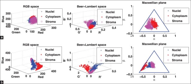
(a-b) Scatter plots in RGB space (left), Beer-Lambert space (center), and Maxwellian plane (right). (a) MILLERS -E. (b) CYTK

Supervised Classification

To assess classification performance, a support vector machine[10,11] was utilized for each stain. Given an image with a particular stain, let {x_i, i = 1, …, n} denote the set of vectors representing the pixel locations in the image (i.e., patterns) where n is the total number of pixels. In the Maxwellian plane, each such vector x_i is in ℝ². For every pair of classes, ω₁, ω₂, a general support vector classifier is defined as ƒ(x) = w^Tɸ(x)+ w₀, where x is a pattern to be classified, w, w₀ are the weights defining the classifier, and ɸ(.) is a mapping of the patterns into kernel space. We have used a radial basis function (RBF) defined by:

K(x_l, x) = exp(–γ||x_l – x||²)

for the support vector classifier, where γ is a parameter that controls the width of the Gaussian kernel. The classifier may be optimized with regard to γ using ten-fold cross-validation; however, the classifier parameters in this case consist not only of γ, but also of a regularization term C, which may be chosen freely (please refer to the Appendix for details). In order to optimize the classifier with regard to both these parameters simultaneously, an exhaustive grid search algorithm[12] ensures arriving at the optimal combination of the (C, γ) values. An example of such an optimization is shown in Figure 3 in the form of a contour plot in which the minimum corresponds to the optimal combination.

Figure 3.

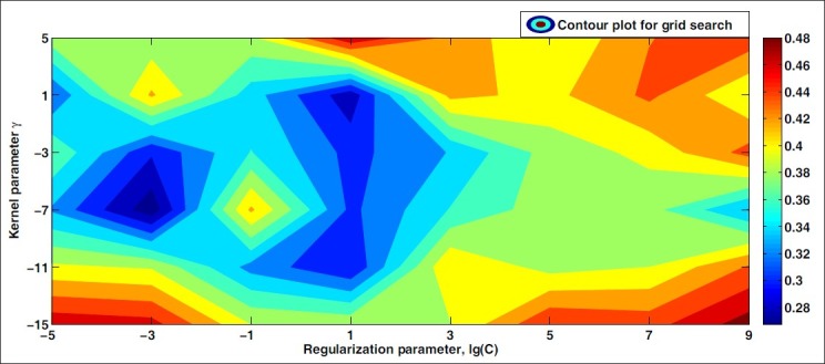
Optimization of SVM radial basis function kernel parameter and regularization parameter C by grid search. Note that lg(.) is the base 2 logarithm

For each stain, we construct a support vector classifier using an RBF kernel that is then optimized as described above, with γ ranging from 2^–15 to 2⁵ and the regularization parameter C ranging from 2^–5 till 2⁹, to ensure coverage of a wide range of simple-to-complex boundaries.[12] We then perform ten-fold cross-validation on each stain using a support vector classifier optimized for that stain. The final result is shown in Figure 4, where the abscissa is ordered according to increasing classification error. We conclude that with respect to supervised classification, the stains MALLORY, CYTK, HERO, GIEMSA, and SIR+ show a considerably better performance for prostate tissue than the other stains. This is attributed to a significant class overlap for the other stains. A stain combination that stains several different structures in the tissue with the same color component is at a disadvantage, as this may lead to a high class overlap and low classification rates.

Figure 4.

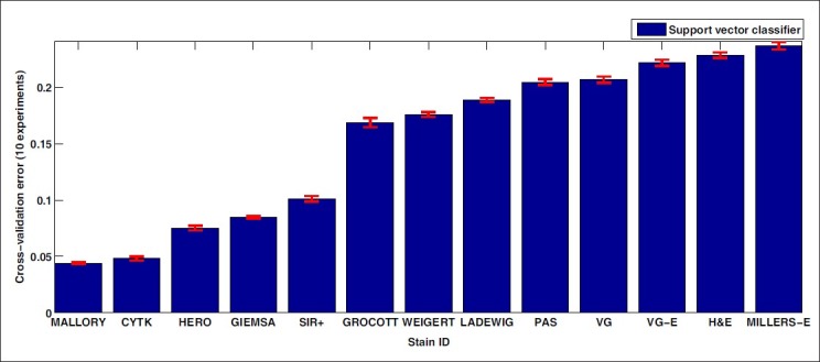
Ten-fold cross-validation error using an optimized SVM classifier for each stain

Unsupervised Classification

Blind classification is sometimes preferred over supervised classification because it avoids manual labeling. Assuming that the class labels are unknown, we assess the clustering performance by the Gaussian mixture model.[13,14] For each class, ω_j, the probability density function is modeled by a Gaussian component completely described by its mean μ_j and covariance matrix ∑_j:

where θ^j is the set of parameters for the distribution of class ω_j, θ_j {μ_j, ∑_j} that is, and d is the number of features, that is, the α and β coordinates in the Maxwellian plane. Thus, the complete dataset may be described as a mixture of these components given by: p(x;ψ) = ∑^K_j=1 α_j·p(x; θ_j) where K is the number of Gaussian components, or clusters, ψ is the total set of parameters for the mixture distribution, and α_j is the prior probability associated with the j^th Gaussian component, and ∑^K_j=1α_j = 1. The expectation-maximization algorithm is used to maximize the log-likelihood, Q, by observing the data given by the Gaussian model. During the expectation step (or E-step) of the algorithm, the cluster membership of each object, w_ji, is computed using the Bayes’ theorem. This is followed by an update of the mixture prior probabilities, α_j, and the cluster means and covariance matrices, ω_j, θ_j {μ_j ∑_j}_{j= 1,…,K} during the maximization step (or M-step). The E-M steps are repeated in succession until convergence, that is, until the change in the log-likelihood function Q is below a tolerance of 10^–10 (see Appendix for details). We initialize the expectation–maximization algorithm with repeated random initializations to obtain the first estimates for the mixture density parameters and select the result with the highest log-likelihood. The results of the Gaussian mixture model clustering for the MALLORY, GIEMSA, SIR+, and CYTK stains, on the prostate tissue samples in Figure 1, are shown in Figure 5. The highlighted contours in the figures correspond to a level 25% below the maximum value of the Gaussian.

Figure 5.

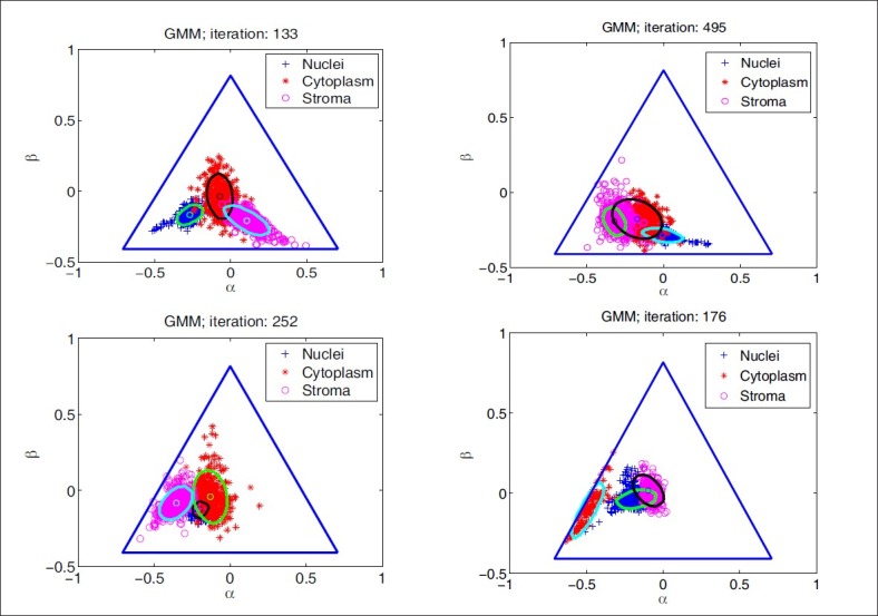
Gaussian mixture model clustering for different stains: Mallory (upper left), Giemsa (upper right), SIR+ (lower left), CYTK (lower right)

To assess clustering performance objectively, we use the class labels from the previous supervised classifications and compute two cluster validation measures, the Rand index[15] and the F-measure[16,17], which are computed pairwise over all the objects in the dataset:

where TP = True Positives, TP = True Negatives, FP = False Positives, and FN = False Negatives, and

where P and R are precision and recall, defined as:

We chose β = 1 to give comparable weights to precision and recall, and the measure is then denoted as an F₁-measure. The result of this analysis is shown in Figure 6. Both performance measures indicate that the five best stains in the supervised case are also more favorable here.

Figure 6.

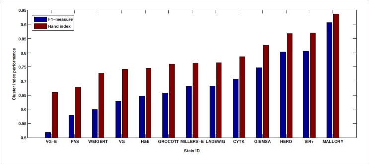
Clustering evaluation using the F₁-measure and Rand index

Class Separability Measures

In order to assess the separability of the classes in terms of how compact and distant they are from each other, we have utilized a Fisher-based criterion[18] and a sum of the squared Mahalanobis distance.[19] We define the Fisher criterion as trace(S^–1_WS_B) where S_W and S_B are the within- and between-scatter matrices:

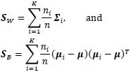
with μ the mean of the entire dataset, and ∑_i and μ_i, the covariance matrix and mean of class ω_i, respectively, n_i the number of patterns in class ω_i, and n the total number of patterns in the dataset. On the other hand, the Mahalanobis distance defined between two classes with means μ₁, μ₂ and covariance matrices ∑₁, ∑₂ is given by:

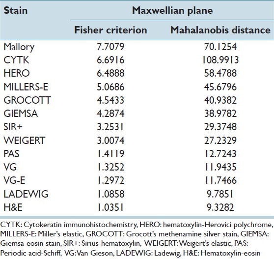
If the classes are compact and well-separated, then they should have a relatively high Mahalanobis distance. We compute the squared Mahalanobis distance for every pair of classes and sum up these values. The result is shown in Table 1, where we see that the optimal stains according to these measures are Mallory's trichrome and Cytokeratin. However, we also see that some of the stains, such as the Miller's elastic, rank well despite their poor classification rate, and this is attributed to the fact that the scatter-based criteria may not always predict the performance of a classifier correctly. A simple example that demonstrates this occurs when two classes are compact, but completely overlapping, and the third class is compact and extremely distant from the other two classes. This third class would influence the result positively, although two of the classes are completely overlapping, and will lead to a low classification rate. One can notice the effect a distant class may have on the Mahalanobis distance by observing the scatter plot of the Cytokeratin stain in the Maxwellian plane [Figure 5], which has led to the high value of the Mahalanobis distance for CYTK in Table 1.

Table 1.

Values for the fisher criterion and sum-of-squared mahalanobis distance for the different stains

DISCUSSION

We have presented a methodology for quantitative comparison of histological stains based on their classification and clustering performance. Among the stains we have investigated, using prostate tissue samples, the classification results suggest that MALLORY, CYTK, HERO, GIEMSA, and SIR+ have an advantage over the other stains, with supervised classification error rates below 11%, and below 5% for MALLORY and CYTK. Furthermore, blind classification was assessed using the Gaussian mixture model and the Rand and F₁-measures. Results show that MALLORY and SIR+ outperform other stains in terms of clustering accuracy, with Rand indices above 0.85. We also saw that simple criteria, such as the Fisher criterion and the Mahalanobis distance, give a good ranking of stains, but may in some cases be misleading. The ideal stain is one where the reference colors are compact and separate, with a good classification performance. Furthermore, with an ideal stain, all tissue types absorb a similar amount of stain, without oversaturation. For the purpose of high-throughput imaging, the choice of a histological stain for a given application must be motivated by the objective criteria that optimize the automation process by facilitating machine learning and image analysis techniques.

APPENDIX

Support Vector Machines

The correct classification of all objects is assumed if the following conditions hold for i = 1, …, n:

where y_i is the class label for object x_i, ξ_i and is the slack variable corresponding to object x_i. These conditions may be rewritten in compact form as

y_i(w^Tɸ(x) + w₀) – 1 + ξ_i ≥ 0, i = 1, …, n.

The support vector classifier aims at maximizing the margin between the classes, which is equivalent to minimizing the norm of the weights. In addition, the slack variables are added to the quantity to be minimized, while regulated by a cost (or regularization) parameter C to allow for class overlap. This minimization is subject to constraints, namely, the patterns are classified correctly, as described above. Thus the classifier minimizes the following criterion:

subject to y_i(w^Tɸ(x) + w₀) – 1 + ξ_i ≥ 0, i = 1, …, n.

This may be formulated using Lagrange multipliers, whereby the following Lagrangian form is obtained:

where α_i is the Lagrange multiplier associated with the constraint equation corresponding to pattern x_i, and r_i is the Lagrange multiplier associated with slack variable ξ_i and ensures that ξ_i remains positive. By differentiating L with respect to the weights and the slack variables, setting the result to zero, and then solving, we obtain the following:

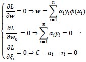
Note that the last result C – α_i – r_i = 0 may be combined with r_i ≥ 0 to give 0 ≤ α_i ≤ C. By substituting these results back into the Lagrangian, we obtain the dual form of the Lagrangian:

Quadratic programming is then employed to solve for the Lagrange multipliers, α_i, i = 1,…, n. Once these are obtained, w is computed from w = ∑_l∈SVα_ly_lɸ(x_l), where SV is the set of support vectors (objects associated with α_i ≠ 0). Thereafter, the offset w₀ is obtained from: α_i(y_i(w^Tɸ(x) * w₀) – 1 + ξ_i) by averaging over objects with 0 < α_i < C, that is, ξ_i = 0. The support vector classifier is then derived as:

ƒ(x) = ∑_l∈SVα_ly_lɸ^T(x_l)ɸ(x) + w₀.

The scalar product ɸ^T(x_l)ɸ(x) is substituted by a kernel function K(x_l, x) = (ɸ^T (x_l)ɸ(x), without the need to explicitly define the transformation function or mapping ɸ(.)

Gaussian Mixture Model

The likelihood of observing the data given by the model for a single component is given by:

If we assume that the class labels are known and are given by:

then the likelihood function may be rewritten as:

The Gaussian mixture model employs the expectation-maximization algorithm to maximize this likelihood or rather log-likelihood function

However, since z_ji is not known, the following function is maximized instead:

During the E-step, the cluster membership of each object, w_ji at any given iteration m becomes:

During the M-step of the algorithm the distribution parameters are updated:

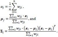
These two steps are repeated iteratively until convergence.

REFERENCES

- 1.Begelman G, Zibulevsky M, Rivlin E, Kolatt T. Blind decomposition of transmission light microscopic hyperspectral cube using sparse representation. IEEE Trans Med Imag. 2009;28:1317–24. doi: 10.1109/TMI.2009.2015145. [DOI] [PubMed] [Google Scholar]
- 2.Gavrilovic M. Doctoral thesis. Uppsala: Acta Universitatis Upsaliensis; 2011. Spectral image processing with applications in biotechnology and pathology. [Google Scholar]
- 3.Tadrous PJ. Digital stain separation for histological images. J Microsc. 2010;240:164–72. doi: 10.1111/j.1365-2818.2010.03390.x. [DOI] [PubMed] [Google Scholar]
- 4.Rabinovich A, Laris CA, Inc Qdm, Agarwal S, Price JH, Belongie S. Unsupervised color decomposition of histologically stained tissue samples. Advances in Neural Information Processing Systems. 2004 [Google Scholar]
- 5.Ruifrok AC, Johnston DA. Quantification of histochemical staining by color deconvolution. Anal Quant Cytol Histol. 2001;23:291–9. [PubMed] [Google Scholar]
- 6.Bancroft JD, Gamble M. Theory and practice of histological techniques. 6th ed. Elsevier: Churchill Livingstone; 2007. [Google Scholar]
- 7.Parson WW. Modern optical spectroscopy. New York: Springer; 2009. [Google Scholar]
- 8.Judd DE. A maxwell triangle yielding uniform chromaticity scales. J Opt Soc Am. 1935;25:24–35. [Google Scholar]
- 9.Foley J, van Dam A, Feiner S, Hughes J. Computer graphics: Principles and practice. Massachusetts: Addison Wesley; 1992. p. 213. [Google Scholar]
- 10.Vapnik V. The Nature of statistical learning theory. New York: Springer-Verlag; 1995. [Google Scholar]
- 11.Bishop C. Pattern recognition and machine learning. New York: Springer; 2006. p. 325. [Google Scholar]
- 12.Hsu CW, Chang CC, Lin CJ. A practical guide to support vector classification. Tech report. Dept of CS and IE, National Taiwan University, Taipei. 2003. [Last accessed on 2012 Sep 4]. Available from: http://www.csie.ntu.edu.tw/cjlin/libsvm/
- 13.Theodoridis S, Koutroumbas K. Pattern Recognition. 4th ed. Massachusetts: Academic Press; 2009. pp. 44–8. [Google Scholar]
- 14.Bishop C. Statistical pattern recognition. New York: Springer; 2006. p. 430. [Google Scholar]
- 15.Rand WM. Objective criteria for the evaluation of clustering methods. J Am Stat Assoc. 1971;66:846–50. [Google Scholar]
- 16.van Rijsbergen CJ. Information retrieval. 2nd ed. London: Butterworths; 1979. [Google Scholar]
- 17.Curic V, Heilio M, Krejic N, Nedeljkov M. Mathematical Model for efficient water flow management. Nonlinear Anal Real World Appl. 2010;11:1600–12. [Google Scholar]
- 18.Webb A. Statistical pattern recognition. 2nd ed. USA: Wiley; 2002. p. 311. [Google Scholar]
- 19.Webb A. Statistical pattern recognition. 2nd ed. USA: Wiley; 2002. p. 414. [Google Scholar]