A marginalized MAP approach and EM optimization for pair-wise registration

Abstract

We formalize the pair-wise registration problem in a maximum a posteriori (MAP) framework that employs a multinomial model of joint intensities with parameters for which we only have a prior distribution. To obtain an MAP estimate of the aligning transformation alone, we treat the multinomial parameters as nuisance parameters, and marginalize them out. If the prior on those is uninformative, the marginalization leads to registration by minimization of joint entropy. With an informative prior, the marginalization leads to minimization of the entropy of the data pooled with pseudo observations from the prior. In addition, we show that the marginalized objective function can be optimized by the Expectation-Maximization (EM) algorithm, which yields a simple and effective iteration for solving entropy-based registration problems. Experimentally, we demonstrate the effectiveness of the resulting EM iteration for rapidly solving a challenging intra-operative registration problem.

1 Introduction

The field of medical image registration has been very active in the past two decades. Although numerous alignment methods have been introduced, only limited attention has been devoted to study the relationship among the available methods and the justification for their preference, implicit and explicit hypothesis and their performance[19, 13]. Currently, a significant number of methods build upon the maximum likelihood framework because of its intuitive nature and ease of implementation. According to this approach, correct alignment is obtained if we find the transformation that makes the the current observations most probable. Recently, with the abundance of available data sets, using prior information to guide registration has received significant attention. Such techniques allow for more robustness and a larger capture range in the implementation, and with respect to the transformation domain, they facilitate the introduction of smoothness constraints on the deformation models.

When relying on prior models, however, it is challenging to find the appropriate balance between previous and current observations. For example, it is not obvious how the level of confidence in the model can be automatically encoded and/or changed over time. Preliminary efforts using both model- and data-related terms have introduced both sequential and unified algorithms with arbitrary weighing terms [4, 9]. In this work, we focus on the establishment of a maximum a posteriori (MAP) framework that allows for making use of prior information about both the transformation and the joint statistics of the observed intensity distributions. By treating the former as nuisance parameters, we can marginalize them out and define our registration goal as a posterior on the transformation components. Depending on how informative the prior is on the joint statistics, we demonstrate implicit relationships with currently used methods. We also introduce an attractive optimization framework over our marginalized formulation – the Expectation-Maximization (EM) algorithm allows us to compute the registration update in a simple and elegant way.

2 Problem Formulation

2.1 Marginalized MAP formulation of registration

Given multi-modal input data sets, u and v, our goal is to find transformation T that that brings those into correct alignment. In addition to the unknown transformation parameters, we introduce another set of parameters, Θ, that encode a discrete joint probability distribution. This model is used in such a way that, if the intensities in the two images are discretized to take values in {I₁, I₂,…, I_K} then the probability of corresponding voxels (at location j) having discrete intensity values of T(u)_j = I_a and v_j = I_b is p(u, v|T) = p(T(u)_j = I_a, v_j = I_b) = Θ(a, b). If we use a simplified, one-dimensional indexing for the parameters of the discrete joint probability model, Θ = {θ₁,…, θ_g} encodes information about intensity joint value occurrences as parameters of an unknown multinomial model, where ∀i θ_i ≥ 0 and ${\sum }_{i=1}^g{\theta }_i=1$. This model can also incorporate any additive noise.

The posterior parameter distribution of the transformation variable T and the joint statistics model Θ with respect to the image observations is p(T, Θ|u, v). In order to align the data sets, this quantity is to be maximized. For our registration purposes though, it is more attractive to compute the posterior on just the transformation parameters. This is manageable given a prior model on the joint statistics parameters that can be marginalized out. Assuming independence between the transformation and the joint distribution models, the posterior distribution of the transformation variable T with respect to solely the image observations is:

$$p(T\mid u,v)\propto \int P(u,v\mid T,\mathrm{\Theta })P(T)P(\mathrm{\Theta })d\theta .$$ (1)

In Eq.(1), the P(u, v|T, Θ) term indicates the likelihood function of the transformation and the model parameters given the input observations, and the rightmost two terms are prior distributions over the T and Θ parameters respectively. Optimizing over such a quantity provides a convenient formulation of the registration objective, if we assume that we have prior knowledge about both the transformation and the joint statistics. The most optimal set of transformation parameters T̂ are then the ones that optimize the following objective function:

$$\widehat{T}=arg\underset{T}{max}logp(T\mid u,v).$$ (2)

2.2 The likelihood term

Using the multinomial model for ordered data, the likelihood of the image observations given the offsetting transformation and an unknown joint probability model is

$$p(u,v\mid T,\mathrm{\Theta })\propto \prod _j{\theta }_j^{n_j(T)},$$ (3)

where n_j(T) is the number of voxel pairs that map to the intensity bin associated with θ_j (i.e. T (u)_j = I_a and v_j = I_b) and ${\sum }_{i=1}^{g}n{(T)}_i=N$ is the total number of observations. Note that the values of n_j depend on the transformation T, and this dependency is made explicit in this notation.

2.3 Prior on the joint statistics model

For the registration problem, the multinomial distribution is a convenient choice of representation as the θ_i parameters naturally correspond to the widely used histogram encoding of the joint statistics of images given g number of components. Additionally, prior information about such parameters can be expressed by using the Dirichlet distribution, the conjugate prior to a multinomial distribution. We choose the following encoding

$$\text{Dirichlet}(\mathrm{\Theta };w)=\frac{1}{Z(w)}\prod _{i=1}^g{\theta }_i^{(w_i-1)}=\mathrm{\Gamma }(w_0)\prod _j\frac{{\theta }_j^{(w_j-1)}}{\mathrm{\Gamma }(w_j)},$$ (4)

where ∀i w_i > 0 and ${\sum }_{i=1}^g{w}_i=w_0$. We may interpret w₀ as the total number of pseudo measurements observed to obtain information about the model and w_i as the individual frequency counts for the joint distribution parameters. The higher the former number is, the greater our confidence becomes in the values of the prior observations.

2.4 The proposed objective function

Using Eq.(3) and Eq.(4), we write the posterior probability on T from Eq.(1) as

$$p(T\mid u,v,w)\propto P(T)\int \left(\prod _i{\theta }_i^{n_i(T)}\right)\mathrm{\Gamma }(w_0)\left(\prod _j\frac{{\theta }_j^{(w_j-1)}}{\mathrm{\Gamma }(w_j)}\right)d\theta$$ (5)

$$\propto P(T)\frac{\mathrm{\Gamma }(w_0)}{\mathrm{\Gamma }(N+w_0)}\left(\prod _j\frac{\mathrm{\Gamma }(n_j(T)+w_j)}{\mathrm{\Gamma }(w_j)}\right),$$ (6)

where we derived Eq.(6) by identifying a Dirichlet distribution with parameters n_j(T)+w_j and using the fact that the integral of the distribution over its domain is equal to one. Therefore, the objective function of our proposed marginalized MAP registration method becomes

$$\widehat{T}=arg\underset{T}{max}log\left[P(T)\frac{\mathrm{\Gamma }(w_0)}{\mathrm{\Gamma }(N+w_0)}\left(\prod _{j=1}^g\frac{\mathrm{\Gamma }(n_j(T)+w_j)}{\mathrm{\Gamma }(w_j)}\right)\right]$$ (7)

$$=arg\underset{T}{max}\left[logP(T)+\sum _{j=1}^{g}log\mathrm{\Gamma }(n_j(T)+w_j)+C\right].$$ (8)

2.5 Special cases: strength of priors

In the following, we demonstrate how our objective function changes with respect to the nature of the prior, and we also examine the equivalence of our novel objective function of Eq.(8) with some widely used methods. These relationships help us better explain why these registration techniques are expected to converge to the correct alignment configuration.

Uninformative Prior

First we choose an uninformative prior. This means that the prior does not favor any solutions a priori and the current observations are going to be solely responsible for the solution to be computed. As an uninformative prior (whose use achieves an equivalence with the maximum likelihood (ML) solution of the problem), we choose to use Jeffreys’ prior [8].These are not affected by any transformations applied to the variables. Accordingly, we set, w₀ = 1 and ∀ i, $w_i=\frac{1}{g}$, or in words, we assume to have only one prior observation, and it is distributed over all the existing bins (where g represents the total number of bins used in the multinomial model). Consequently,

$$logp(T\mid u,v,w)\to logP(T)+\sum _{j}log\mathrm{\Gamma }\left(n_j(T)+\frac{1}{g}\right)+\text{C}.$$ (9)

The information theoretic joint entropy [6], measuring uncertainty related to the joint occurrence of the input random variables, is defined by:

$$\text{H}\left(\frac{\text{n}}{\text{N}}\right)\equiv -\sum _{\text{j}}\frac{{\text{n}}_{\text{j}}}{\text{N}}\text{log}\frac{{\text{n}}_{\text{j}}}{\text{N}}=-\frac{1}{\text{N}}\sum _{\text{j}}{\text{n}}_{\text{j}}log{\text{n}}_{\text{j}}+\text{log}\text{N},$$ (10)

where Σ_jn_j = N. For the most part, the differences between expressions (Σ_j n_j log(n_j)) and (Σ_j log Γ (n_j)) are small (“first order” version of the Stirling approximation). Therefore, we may re-write the registration objective function using an uninformative prior as

$$\widehat{T}=arg\underset{T}{max}logp(T\mid u,v,w)\approx arg\underset{T}{min}\left[c\text{H}\left(\frac{\text{n(T)}+\frac{1}{\text{g}}}{\text{N}+1}\right)-log\text{P}(\text{T})\right].$$ (11)

This approximation, ignoring the transformation prior, is equivalent to the widely used minimization of joint entropy method [15]. Although widely used, the justification of using that metric in registration has long been debated. Formally, joint entropy is maximum likelihood method. While others have discussed a similar equivalence between ML and joint entropy [18], the present marginalization approach provides a rigorous demonstration of its validity.

Informative Prior

When the priors are informative, or in words, when we have access to a sufficient number of pseudo observations (w_j) from, for example, training data sets, they allow for a more certain belief in their information content. In such a case, the objective function can be approximated by

$$\widehat{T}=arg\underset{T}{max}logp(T\mid u,v,w)\approx arg\underset{T}{min}\left[\text{H}\left(\frac{\text{n(T)}+\text{w}}{\text{N}+{\text{w}}_{\text{0}}}\right)-log\text{P}(\text{T})\right].$$ (12)

According to Eq.(12), prior information is introduced into the framework by pooling together corresponding samples from the previously aligned (prior distribution model) and from the current, to-be-aligned cases. Throughout the optimization, the model observations remain fixed and act as anchor points to bring the other samples into a more likely configuration. Interestingly, this formulation is closely related to another type of entropy-based registration algorithm. Sabuncu et al. introduced a registration technique based on minimizing Renyi entropy, where the entropy measure is computed via a non-plug-in entropy estimator on pooled data [14]. This estimator is based upon constructing the EMST (Euclidean Minimum Spanning Tree) and using the edge length in that tree to approximate the entropy. The reason that such an arrangement would provide a favorable solution has not been previously theoretically justified.

Strong Prior

Lastly, we briefly mention the scenario, where the prior information is very strong.

$$logp(T\mid u,v,w)\approx logP(T)+\sum _j\left(log\mathrm{\Gamma }(w_j)+n_j(T)\frac{{\mathrm{\Gamma }}^{\prime }(w_j)}{\mathrm{\Gamma }(w_j)}\right)+\text{C}$$ (13)

$$\approx logP(T)+\sum _j(w_{j}log(w_j)+n_j(T)log(w_j))+\text{C}.$$ (14)

In Eq.(13) a first order approximation of log Γ(n_j(T)+w_j) around w_j was written out, with Γ′ indicating the derivative of the Gamma function. In Eq.(14), the approximation for Σ_j log Γ (w_j) from Eq.(11) and $\frac{{\mathrm{\Gamma }}^{\prime }(n)}{\mathrm{\Gamma }(n)}\approx log(n)$ are used, where the latter is valid for a large range of n. The only term that depends on n_j(T) is Σ_j n_j(T) log(w_j), thus

$$\widehat{T}=arg\underset{T}{max}logp(T\mid u,v,w)\approx arg\underset{T}{min}\left[logP(T)+\sum _j(n_j(T)log(w_j))\right].$$ (15)

If we re-express the sum in Eq.(15) as a sum over data points, we can see that this formulation is equivalent to an approximate maximum likelihood approach, where the current samples are, indeed, evaluated under the previously constructed model distribution [10]. Chung et al. experimentally showed that the performance of this similarity measure is not always sufficiently accurate[5]. That finding is now explained by the fact that this objective function considers the model with such a high level of confidence that might not be justified by the number of previous observations.

3 EM optimization for the marginalized MAP registration problem

The above described objective functions could be optimized in several ways. In general, we can differentiate between gradient- and non-gradient-based techniques. Using gradient-based information in the optimization procedure often results in significant computational advantages, however, they might also require challenging approximation of some terms. For example, when using the multinomial model, update terms need to be estimated from a discrete distribution and also it is required to calculate the partial derivative of changing (non-fixed) joint statistics parameters with respect to the to-be-optimized transformation components. Although close approximations exist, one might worry about their accuracy. To escape such computational difficulties, we might optimize both of the above marginalized formulations by using the Expectation-Maximization (EM) algorithm [7]. This framework, from the statistical computing literature, is known to have good properties as an optimizer and the resulting iteration is attractive from a practical standpoint. If we consider the input images as observations and the Θ parameters as hidden information, the EM algorithm defines the solution to T̂ = arg max_T log p(T |u, v) as iteratively obtaining the best current solution (T̂_next) based upon:

$${\widehat{T}}_{\text{next}}=arg\underset{T}{max}{\text{E}}_{\mathrm{\Theta }\mid u,v,{\widehat{T}}_{\text{old}}}[logP(T,\mathrm{\Theta }\mid u,v)]$$ (16)

$$=arg\underset{T}{max}{\text{E}}_{\mathrm{\Theta }\mid u,v,{\widehat{T}}_{\text{old}}}[logP(T\mid u,v,\mathrm{\Theta })+logP(\mathrm{\Theta })]$$ (17)

$$=arg\underset{T}{max}{\text{E}}_{\mathrm{\Theta }\mid u,v,{\widehat{T}}_{\text{old}}}\left[log(P(u,v\mid T,\mathrm{\Theta })P(T))+\sum _{j=1}^g(w_j-1)log{\theta }_j\right],$$ (18)

where Bayes rule was applied in order to express the conditional probability term on the registering transformation. Continuing with the manipulation

$${\widehat{T}}_{\text{next}}=arg\underset{T}{max}{\text{E}}_{\mathrm{\Theta }\mid u,v,{\widehat{T}}_{\text{old}}}\left[log\prod _j{\theta }_j^{n_j(T)}+logP(T)+\sum _{j=1}^g(w_j-1)log{\theta }_j\right]$$ (19)

$$=arg\underset{T}{max}\left[logP\text{(}T\text{)}+{\text{E}}_{\mathrm{\Theta }\mid u,v,{\widehat{T}}_{\text{old}}}\left[\sum _{j=1}^g(n{(T)}_j+w_j-1)log{\theta }_j\right]\right]$$ (20)

$$=arg\underset{T}{max}\left[logP\text{(}T\text{)}+\sum _{j=1}^g(n{(T)}_j+w_j-1){\text{E}}_{\mathrm{\Theta }\mid u,v,{\widehat{T}}_{\text{old}}}[log{\theta }_j]\right]$$ (21)

If we define l_j = log θ_j, then we can define the two steps of the EM algorithm: maximization (M) and expectation (E) as follows:

$$\mathbf{M}-\mathbf{step}:{\widehat{T}}_{\text{next}}=arg\underset{T}{max}\left[logP(T)+\sum _{j=1}^g(n{(T)}_j+w_j-1)l_{j_{\text{old}}}\right]$$ (22)

$$\mathbf{E}-\mathbf{step}:l_{j_{\text{next}}}=E_{\mathrm{\Theta }\mid u,v,{\widehat{T}}_{\text{old}}}[l_j],$$ (23)

In words, the M-step searches for transformation T that optimizes the sum of expectation over the log model parameters and a transformation prior; and the E-step calculates the expectation of these log parameters given the current best estimate of the transformation parameters. Note that in this framework, we need to pay special attention to the scenario where the θ_j parameters tend to zero and we also have to enforce the property that the parameters add to one. More details on these special cases are discussed below.

3.1 Evaluating the E-step

In order to evaluate the expression in the E-step, we may use the following form for the posterior on Θ given the input images and the transform:

$$P(\mathrm{\Theta }\mid u,v,T)=\frac{P(u,v\mid \mathrm{\Theta },T)P(\mathrm{\Theta })}{{\int }_{\mathrm{\Theta }}P(u,v\mid \mathrm{\Theta },T)P(\mathrm{\Theta })d\theta }.$$ (24)

Computing the expectation term thus becomes:

$${\text{E}}_{\mathrm{\Theta }\mid u,v,\widehat{T}}[log{\theta }_l]={\int }_{\mathrm{\Theta }}log{\theta }_{l}P(\mathrm{\Theta }\mid u,v,\widehat{T})d\theta ={\int }_{\mathrm{\Theta }}log{\theta }_l\frac{P(u,v\mid \mathrm{\Theta },\widehat{T})P(\mathrm{\Theta })}{{\int }_{\mathrm{\Theta }}P(u,v\mid \mathrm{\Theta },\widehat{T})P(\mathrm{\Theta })d\theta }d\theta .$$ (25)

Using our multinomial model and the Dirichlet distribution as its prior, the numerator in Eq.(25) has the form of another unnormalized Dirichlet distribution. Therefore, if we define a new Dirichlet distribution with parameters β, where β_i = (n(T̂)_i + w_i), we may write

$${\text{E}}_{\mathrm{\Theta }\mid u,v,\widehat{T}}[log{\theta }_l]={\int }_{\mathrm{\Theta }}log{\theta }_l\frac{{\prod }_{j=1}^g{\theta }_j^{n{(\widehat{T})}_j}\frac{1}{Z(w_0)}{\prod }_{k=1}^g{\theta }_k^{(w_k-1)}}{{\int }_{\mathrm{\Theta }}{\prod }_{j=1}^g{\theta }_j^{n{(\widehat{T})}_j}\frac{1}{Z(w_0)}{\prod }_{k=1}^g{\theta }_k^{(w_k-1)}d\theta }d\theta$$ (26)

$$={\text{E}}_{\text{Dir}(\mathrm{\Theta };\beta )}[log{\theta }_l].$$ (27)

The expression in Eq.(27) is the expected value of the (log θ_l) parameters given a Dirichlet distribution parameterized by β. As the Dirichlet distribution belongs to the family of exponential functions, the expectation over its sufficient statistics can be computed as the derivative of the logarithm of the normalization factor with respect to its natural parameters[2]. Writing the Dirichlet distribution in its exponential form results in

$$\text{Dir}(\mathrm{\Theta };w)=exp\left(\sum _{i=1}^g(w_i-1)log{\theta }_i+log\mathrm{\Gamma }(w_0)-\sum _{i=1}^{g}log\mathrm{\Gamma }(w_i)\right).$$ (28)

Given this form, we see that the sufficient statistics are indeed the (log θ_l) parameters. Therefore, the expectation term we are concerned with can be expressed by using the Digamma (or Psi) function which is the first derivative of the log Gamma functions [11].

$${\text{E}}_{\text{Dir}(\mathrm{\Theta };\beta )}[log{\theta }_l]=\mathrm{\Psi }({\beta }_l)-\mathrm{\Psi }({\beta }_0)=\mathrm{\Psi }(n{(\widehat{T})}_l+w_l)-\mathrm{\Psi }(N+w_0).$$ (29)

In the following, we approximate the Digamma expressions in Eq.(29) by using Ψ(x) ≈ log(x − .5) [1]. This approximation is very accurate in the positive real domain, except for values in the range of [0, 1]. A value in that particular range would correspond to the extreme scenario of an “empty bucket”, where there are neither current nor prior observations associated with a particular model parameter. In order to make the approximation hold even in such a scenario, we differentiate between two cases: uninformative and informative priors. In the case of uninformative priors, we propose to use Laplace priors [8] instead of zero counts for the Dirichlet parameters. Consequently, when no prior/pseudo information is available for the model, we initialize all parameters uniformly as one. The case of informative priors requires more attention. Although the total sum of pseudo information in this case is significant, we cannot directly assume that it holds for all individual Dirichlet parameters. Thus in that case we explicitly require that each pseudo count should hold at least one count. With such specifications we can ensure that our approximation holds regardless of the nature of the prior information and that the argument of the log function, in the case of the parameter update, does not approach zero (which could be a concern as mentioned while defining the EM framework). Thus the E-step of the EM algorithm is expressed as

$${({\overline{l}}_l)}_{\text{next}}=\mathrm{\Psi }\left(n{({\widehat{T}}_{\text{old}})}_l+w_l\right)-\mathrm{\Psi }(N+w_0)$$ (30)

$$\approx log\left(n{({\widehat{T}}_{\text{old}})}_l+w_l-.5\right)-log(N+w_0-.5)$$ (31)

$$=log\left(\frac{n{({\widehat{T}}_{\text{old}})}_l+w_l-.5}{N+w_0-.5}\right).$$ (32)

This rule assigns the logarithm of normalized sum of the pseudo and observed counts minus a constant to the most current log(θ) parameters. This pooling of current and pseudo counts for describing joint intensity statistics has been already discussed in Sec. 2.5. We point out that, in order to enforce the relationship ${\sum }_{i=1}^g{\theta }_i=1$, we compute the E-step for all 1 ≤ j ≤ (g − 1) and we assign the last remaining parameter as ${({\overline{l}}_g)}_{\text{next}}=log\left[1-{\sum }_{i=1}^{g-1}exp({({\overline{l}}_i)}_{\text{next}}\right]$.

3.2 Evaluating the M-step

Using the results from the E-step, we may now express the M-step (the most current estimate of the registration parameter), which indeed results in a simple formulation of the problem:

$${\widehat{T}}_{\text{next}}=arg\underset{T}{max}{\text{E}}_{\mathrm{\Theta }\mid u,v,{\widehat{T}}_{\text{old}}}[logP(u,v,\mathrm{\Theta }\mid T)]$$ (33)

$$=arg\underset{T}{max}\left[\mathit{logP}(T)+\sum _{j=1}^g(n{(T)}_j+w_j-1){\text{E}}_{\mathrm{\Theta }\mid u,v,{\widehat{T}}_{\text{old}}}[l_j]\right]$$ (34)

$$=arg\underset{T}{max}\left[logP(T)+\sum _{j=1}^g(n{(T)}_j+w_j-1)log\left(\frac{n{({\widehat{T}}_{\text{old}})}_j+w_j-.5}{N+w_0-.5}\right)\right]$$ (35)

$$=arg\underset{T}{max}\left[logP(T)+\sum _{j=1}^{g}n{(T)}_{j}log\left(n{({\widehat{T}}_{\text{old}})}_j+w_j-.5\right)\right]$$ (36)

Therefore, ignoring the prior on transformation T, our objective function in the M-step is the maximization of a log likelihood term. When solving the optimization problem with a non-informative set of priors, the solution approaches an iterated ML framework. This result underlies the fact that an MAP framework with a non-informative prior produces results that are equivalent to the ML solution. The best transformation parameters therefore are calculated by using old, currently the best, model estimates. In the scenario where we have significant amount of prior information with respect to the model, again, the pseudo and the current observations are pooled together.

We note that the expression in Eq.(36) can be further simplified to result in an information theoretic framework that comprises of a data- and model-related term. The former measures the KL-divergence between two categorical distributions over the parameters describing the current joint statistics and that including pseudo observations from the prior model and the latter computes the entropy of the estimated joint statistics of the observations.

$${\widehat{T}}_{\text{next}}\approx arg\underset{T}{max}\left[logP(T)-{\text{D}}_{\text{KL}}\left(n(T)\left|\right|n({\widehat{T}}_{\text{old}})w_j-.5\right)-\text{H}(\text{n}(\text{T}))\right]$$ (37)

$$\approx arg\underset{T}{min}\left[{\text{D}}_{\text{KL}}\left(p_T\left|\right|p_{{\widehat{T}}_{\text{old},w}}\right)+\text{H}({\text{p}}_{\text{T}})-log\text{P}(\text{T})\right]$$ (38)

In summary, the utilization of the EM framework provides an iterative method for the transformation parameter estimation where the model parameter updates are computed in an efficient and principled manner.

4 Experimental results

In this section, we present our experimental results from an iterated registration algorithm that uses uninformative priors. The resulting EM solution to the ML (in θ) formulation is demonstrated on a complex intra-operative non-rigid brain registration problem. We introduced a prior on the deformation field that approximates a fluid flow model. The algorithm also facilitates (on the EM iterations) a quadratic approximation to the search problem that may be quickly solved. That would not be justified if the multinomial model were not constant within the iterations. Preliminary experimental results for the scenario where we do have access to informative prior information was presented in [20]. At each iteration, our non-rigid registration algorithm defines the prior probability on configurations phenomenologically, using linear elastic deformation energy and Boltzmann’s Equation, as P(T) ∝ exp(−E/τ). Configurations of the deforming anatomy are parameterized by the coordinates of the vertices of an adaptive tetrahedral mesh. Using standard methodology of the Finite Element Method (FEM) [17], the stress-strain integral is linearized about the current configuration, yielding a quadratic approximation for the energy in terms of displacements from the current configuration, $E\approx {\mathrm{\Delta }}_T^{T}K{\mathrm{\Delta }}_T$, where K is a banded elasticity matrix. At each iteration, the log likelihood, log P(n(T)_old|Δ_T), is approximated by a second order Taylor expansion. This is centered on a nearby local maximum of the likelihood function that we locate using a greedy method. The resulting quadratic expression is combined with the quadratic prior term, and the resulting approximation to the posterior probability is easily solved as a linear system. This iterative method resets the elastic energy to zero at each iteration. Papademetris et al. [12] call this “history free” approach the incremental approach, and point out that, in a limiting case, it is equivalent to the fluid model [3].

Figures 1(a) and (b) show two MRI images of the same brain taken during brain surgery. The images contain 256×256×124 voxels with 0.9375×0.9375×1.5 mm spacing. According to visual comparison, deformation between the two images mostly occurs near the incision. The result of the non-rigid registration algorithm is shown in Fig. 1(c). The warped image is very similar to the target image. In particular, the small displacement of the left and right ventricles was captured and the boundaries near the incision appear to be in appropriate places as well. The final match used 8500 mesh nodes, and the entire matching process was finished in less than 6 minutes on a 2 Ghz desktop computer. To validate our registration results, we compared manually located landmarks in the initial and the deformed images. The majority of the motion was captured by our non-rigid registration algorithm, with disagreements typically not more than the voxel size. More details on the experimental setup and the validation results is described in dissertation work [16].

Fig. 1.

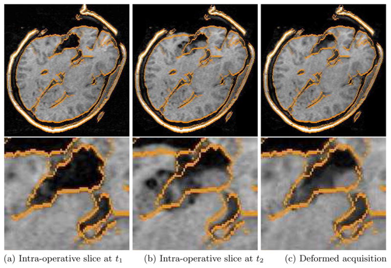
MRI acquisition of the brain: (a) taken during surgery with edges highlighted; (b) taken later in the surgery, with the edges from (a) overlaid; (c) deformed the former image onto the latter, with the edges of (a) overlaid.

5 Conclusion

We introduced an MAP framework for the pair-wise registration problem that allowed us to include prior information about not only the transformation parameter space but also the joint intensity statistics of the inputs. Treating the latter as nuisance parameters and marginalizing them out allowed us to establish a close relationship between our method and certain entropy-based objective functions. We also demonstrated that using an EM-based optimization framework the aligning transformations can be computed in a principled and computationally attractive manner.

References

- 1.Abramowitz M, Stegun IA. Handbook of Mathematical Functions. New York: Dover; 1964. [Google Scholar]
- 2.Blei DM, Ng AY, Jordan MI. Latent dirichlet allocation. Journal of Machine Learning Research. 2003;3:993–1022. [Google Scholar]
- 3.Christensen GE, Rabbit RD, Miller MI. Deformable templates using large deformation kinematics. IEEE Transactions on Image Processing. 1996;5(10):1435–1447. doi: 10.1109/83.536892. [DOI] [PubMed] [Google Scholar]
- 4.Chung ACS, Gan R, Wells W. Robust multi-modal image registration based on prior joint intensity distributions and minimization of kullback-leibler distance. Technical Report HKUST-CS07-01, HKUST. 2007 [Google Scholar]
- 5.Chung ACS, Wells WMW, III, Norbash A, Grimson WEL. MICCAI, volume 2 of LNCS. Springer; 2002. Multi-modal Image Registration by Minimizing Kullback-Leibler Distance; pp. 525–532. [Google Scholar]
- 6.Cover TM, Thomas JA. Elements of Information Theory. John Wiley & Sons, Inc; New York: 1991. [Google Scholar]
- 7.Dempster AP, Laird NM, Rubin D. Maximum likelihood from incomplete data via the em algorithm. Journal of the Royal Statistical Society. 1977;39(1):1–38. [Google Scholar]
- 8.Gelman A, Carlin JB, Stern HS, Rubin DB. Bayesian Data Analysis. CRC Press LLC; Boca Raton, FL: 2003. [Google Scholar]
- 9.Gütter C, Xu C, Sauer F, Hornegger J. Learning based non-rigid multimodal image registration using kullback-leibler divergence. In: Gerig G, Dun-can J, editors. MICCAI, volume 2 of LNCS. Springer; 2005. pp. 255–263. [DOI] [PubMed] [Google Scholar]
- 10.Leventon M, Grimson WEL. MICCAI, LNCS. Springer; 1998. Multi-modal Volume Registration Using Joint Intensity Distributions; pp. 1057–1066. [Google Scholar]
- 11.Minka T. Estimating a dirichlet distribution. Notes. 2003 [Google Scholar]
- 12.Papademetris X, Onat ET, Sinusas AJ, Dione DP, Constable RT, Duncan JS. Proceedings of IPMI, volume 0558 of LNCS. Springer; 2001. The active elastic model; pp. 36–49. [Google Scholar]
- 13.Roche A, Malandain G, Ayache N. Unifying maximum likelihood approaches in medical image registration. International Journal of Imaging Systems and Technology. 2000;11(7180):71–80. [Google Scholar]
- 14.Sabuncu MR, Ramadge PJ. Graph theoretic image registration using prior examples. Proceedings of European Signal Processing Conference; Sept 2005. [Google Scholar]
- 15.Studholme C, Hill DLG, Hawkes DJ. An overlap invariant entropy measure of 3d medical image alignment. Pattern Recognition. 1999;32(1):71–86. [Google Scholar]
- 16.Timoner S. PhD thesis. Massachusetts Institute of Technology; Jul, 2003. Compact Representations for Fast Nonrigid Registration of Medical Images. [Google Scholar]
- 17.Zenkiewicz OC, Taylor RL. The Finite Element Method, Fourth Edition. McGraw-Hill; Berkshire, England: 1989. [Google Scholar]
- 18.Zhu YM, Cochoff SM. Likelihood maximization approach to image registration. IEEE Transactions on Image Processing. 2002;11(12):1417–1426. doi: 10.1109/TIP.2002.806240. [DOI] [PubMed] [Google Scholar]
- 19.Zöllei L, Fisher J, Wells W. Proceedings of IPMI, volume 2732 of LNCS. Springer; 2003. A unified statistical and information theoretic framework for multi-modal image registration; pp. 366–377. [DOI] [PubMed] [Google Scholar]
- 20.Zöllei L, Wells W. Biomedical Image Registration, WBIR. Vol. 4057. Springer; Jun, 2006. Multi-modal image registration using dirichlet-encoded prior information; pp. 34–42. [Google Scholar]