On the Use of Adjusted Cross-Sectional Estimators of HIV Incidence

Abstract

Objective

To elucidate when and how cross-sectional estimators of HIV incidence rates based on a sensitive and less-sensitive diagnostic test should be adjusted.

Methods

Evaluate the statistical properties of unadjusted and adjusted cross-sectional estimators of HIV incidence, including the adjusted estimators considered by McDougal et al, for the 2 settings where (a) all infected subjects eventually become reactive to the less-sensitive test, and (b) a subset of infected subjects indefinitely remain non-reactive to the less-sensitive test. Derive the maximum likelihood estimator of incidence for the latter setting, and use analytical results and simulation studies to compare the performance of the various estimators.

Results

When every infected subject would eventually become reactive to the less-sensitive test, the McDougal adjusted estimator is uniformly less precise than the unadjusted estimator and more susceptible to bias. When a subset of the infected population would indefinitely remain non-reactive to the less-sensitive test, the McDougal adjusted estimator is less precise than the maximum likelihood estimator, which coincides with an estimator developed by McWalter and Welte using a mathematical modeling approach. When the assumed model is incorrect, the unadjusted estimator overestimates incidence whereas the maximum likelihood estimator can be biased in either direction.

Conclusion

The standard unadjusted cross-sectional estimator of HIV incidence should be used when all infected individuals would eventually become reactive to the less-sensitive test. When a subset of individuals would indefinitely remain non-reactive to the less-sensitive test, the maximum likelihood estimator for this setting should be used. Characterizing the proportion of individuals who would indefinitely remain non-reactive is crucial for accurate estimation of HIV incidence.

Introduction

Reliable estimates of HIV incidence rates are critical for tracking the epidemic and planning prevention studies. Several recent prevention studies have led to equivocal results because biased estimates of incidence were used in their planning¹. Cross-sectional methods for estimating HIV incidence rates, using a sensitive (e.g., ELISA) combined with a less-sensitive (e.g., Vironostika de-tuned ELISA or BED capture enzyme immunoassay) diagnostic test, offer important advantages to traditional longitudinal follow-up studies in terms of cost, time, and attrition.² However, as several reports have cautioned, the reliability of cross-sectional methods is in doubt, in part because of inconsistencies between estimates they have produced and those obtained by traditional longitudinal cohort studies.^3,4 These concerns have led some investigators to propose adjustments to the standard estimator.^5,6,7,8 Recently, Brookmeyer has questioned the need for adjusted estimators by arguing that ‘false negatives’ and ‘false positives’ cancel out, thus leading to no essential change.⁹ This raises fundamental questions of when adjustment of the standard estimator is needed and how such adjustments should be made.

One purpose of this paper is to shed light on the choice of incidence estimators by providing intuition behind the McDougal adjustments and demonstrating that, even in the idealized situation when the sensitivity and specificity of the less sensitive test are fully known, these estimators are less precise than the unadjusted estimator in settings where all infected subjects eventually become reactive to the less-sensitive test. A second purpose of the paper is to determine the statistical properties of adjusted estimators of HIV incidence rate when a subset of infected subject would never become reactive to the less-sensitive test. We derive the maximum likelihood estimator of HIV incidence based on a statistical model for this setting. The resulting estimator coincides with one developed by McWalter and Welte⁷ using a mathematical modeling approach. We demonstrate that the precision of the maximum likelihood estimator is always greater than that of the adjusted estimators considered by McDougal et al, and we develop a variance expression for this estimator. Finally, we determine and illustrate the biases of the unadjusted and adjusted incidence estimators when incorrect assumptions are made about a subpopulation of infected subjects who indefinitely remain non-reactive to the less-sensitive test.

Methods

We use longitudinal natural history statistical models of HIV seroconversion and subsequent reactivity to a less-sensitive diagnostic test to determine the statistical properties of unadjusted and adjusted incidence estimators based on a cross-sectional sample. The method of maximum likelihood estimation is used to derive the optimal cross-sectional estimator of HIV incidence for settings where a subset of the infected persons indefinitely remain non-reactive to the less-sensitive test. The bias and precision of the various incidence estimators are assessed and compared using analytic methods, and are illustrated using simulation studies.

Results

3-State Model for HIV Seroconversion and Reactivity to Less Sensitive Test

Suppose that N subjects are randomly selected from an asymptomatic population, and each is tested with an ELISA and, if positive, a less-sensitive antibody test. The most commonly-used less-sensitive tests to date have been the 3A11-LS and Vironostika detuned ELISA assays, and the BED capture enzyme immunoassay.^2,10,11 Let N₁, N₂, and N₃ denote the resulting numbers of subjects found to be non-reactive to ELISA, reactive to ELISA but non-reactive to the less-sensitive test, and reactive to the less-sensitive test, respectively, so that N = N₁ + N₂ + N₃.

Assume that the observations arise from the 3-state longitudinal model depicted in Figure 1. State 1 denotes the pre-seroconversion period when an individual is either uninfected or infected without yet having seroconverted. State 2 denotes the time interval following seroconversion while an individual is non-reactive to the less-sensitive diagnostic test (for example, with a normalized optical density (OD) value below a cutoff of 1.0 with the BED capture enzyme immunoassay), and is sometimes referred to as the “recent infection” state. State 3 denotes the period beginning when the individual would test positive (reactive) with the less-sensitive test, and has been referred to as the “non-recent infection” state.

Figure 1.

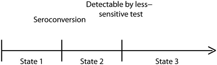
Three-State Model in which All Infected Persons Would Eventually Become Reactive to the Less-Sensitive Test.

Implicit in Figure 1 is the assumption that all infected individuals would eventually become reactive to the less-sensitive test. The actual time spent in State 2, say L, varies from person to person, and is assumed to be independent of time of seroconversion. Because of the inter-person variability in L, use of “recent infection state” to describe State 2 is not meant in any strict literal sense, such as “infected in the past 6 months”. We use μ = E(L), commonly called the “mean window period”, to denote the mean population time in State 2. The distribution of L, and thus the value of μ, will depend on the less-sensitive test being used. For example, Janssen et al, Parekh et al, and Constantine et al report estimated mean window periods of 129, 160, and 133 days for the 3A11-LS assay (using a OD cutoff of 0.75), the BED assay (using a 1.0 normalized OD cutoff), and Vironostika detuned ELISA (using a SOD cutoff of 0.75), respectively.^2,10,11

Unadjusted Incidence Estimators

Suppose that I denotes the population incidence rate at the time of the cross-sectional sample, and consider the unadjusted cross-sectional estimator

$$\widehat{I}=\frac{N_2}{N_1\mu }.$$ (1)

For the moment, we assume that μ is known. This estimator arises as a special case of the snapshot estimator considered Kaplan and Brookmeyer (equation 10)¹². It also arises as the maximum likelihood estimator of I for 4-stage model considered by Balasubramanian and Lagakos¹³ when the time between infection and serconversion is negligible and when the incidence density is constant for a period of time preceding the cross-sectional sample. Because (1) is the maximum likelihood estimator of I in this setting, it follows that as N becomes large, it will converge to the true incidence rate and be the most efficient cross-sectional estimator of incidence. The denominator of Î differs slightly from that in the unadjusted estimator used by Brookmeyer and Quinn¹⁴ and Janssen et al¹, who use N₁ + N₂ instead of N₁. However, N₁ is typically about 2 orders of magnitude larger than N₂, in which case the difference between these versions of the unadjusted estimator is negligible.

Adjusted Incidence Estimators

Adjusted versions of the estimator in (1) have been proposed by several investigators.^5,6,7,8 McDougal et al (equations 1 and 2) consider the estimators

$${\widehat{ℐ}}_1=\frac{{\widehat{\mathcal{N}}}_{2L}}{N_1\mu },$$ (2)

where

$${\widehat{\mathcal{N}}}_{2L}=\frac{N_2-(N-N_1)(1-\text{spec})}{\text{sens}+\text{spec}-1},$$ (3)

and

$${\widehat{ℐ}}_2=\frac{{\stackrel{\sim }{\mathcal{N}}}_{2L}}{N_1\mu },$$ (4)

where

$${\stackrel{\sim }{\mathcal{N}}}_{2L}=\frac{N_2-(N-N_1)(1-{\text{spec}}_{\text{2}})}{\text{sens}-{\text{spec}}_1+2{\text{spec}}_2-1}.$$ (5)

Here sens, spec, spec₁, and spec₂ denote the specificity and sensitivity of the less-sensitive test as regards identifying subjects as having seroconverted within the past μ days; that is, if Y denotes the time between seroconversion and testing,

$$\text{sens}=P(\text{non-reactive on the less-sensitive test}|\text{ELISA}+,Y\le \mu ),$$

$$\text{spec}=P(\text{reactive on the less-sensitive test}|\text{ELISA}+,Y>\mu ),$$

$${\text{spec}}_1=P(\text{reactive on the less-sensitive test}|\text{ELISA}+,\mu <Y\le 2\mu ),$$

and

$${\text{spec}}_2=P(\text{reactive on the less-sensitive test}|\text{ELISA}+,Y>2\mu )$$

Based on longitudinal studies which give similar estimates for sens and spec₁, Hargrove et al⁶ recommend a simplified version of (4) obtained by setting sens=spec₁. However, Brookmeyer⁹ notes that for the model in Figure 1, sens=spec₁ implies that spec₂ = 1, which contradicts Hargrove et al's use of a value of spec₂ less than 1. Welte et al⁸ recommend replacing the denominator in (4) by sens₂, based on analysis of a mathematical model which leads to sens − spec₁ + spec₂ = 1. We return to these estimators later in the paper.

Appendix 1 derives expressions for sens, spec, spec₁, and spec₂ in terms of HIV incidence and prevalence at the time of the cross-sectional sample and the distribution of time in State 2, based on the 3-state model in Figure 1.

To gain insight into the adjusted estimators, imagine a hypothetical less-sensitive test that becomes reactive exactly μ time units after every individual seroconverts. That is, the time, L, in State 2 equals μ for every individual, and every subject found to be in State 2 is a “recent infection” in the literal sense of having seroconverted within the past μ time units. Suppose that N_2L denotes the number of such subjects from the sample of N subjects. Then from the same theory justifying (1), another valid estimator of the HIV incidence rate I would be

$$\frac{{\mathcal{N}}_{2L}}{N_1\mu }.$$ (6)

Furthermore, since N_2L has the same binomial distribution as N₂, the estimator in (6), while giving different numerical results than the unadjusted estimator in (1) for a given data set, has the same distribution and thus is equally precise. Of course, this estimator cannot be used because no such hypothetical less-sensitive test exists. However, the adjusted estimators (2) and (4) can be viewed as approximations of (6) based on replacing the unobservable quantity N_2L by N̂_2L and Ñ_2L, respectively. It is shown in Appendix 2 that for the 3-state model in Figure 1, N̂_2L and Ñ_2L have the same expectation as N₂ and that ₁ and ₂ are valid estimators of I; that is, will converge to I as N grows large. This result is analogous to the finding by Brookmeyer, who shows that the “false positives” and “false negatives” cancel out in the adjustment formula considered by McDougal et al, and forms the basis for his conclusion that “The McDougal adjustment has no net effect”.⁹

One key point is that, because (2) and (4) are based on estimates of N_2L, the variances of ₁ and ₂ are always larger than that of Î (Appendix 3). Another is that the estimators in (2) and (4) cannot be computed in practice because sens, spec, spec₁, and spec₂ are not known exactly. That is, the adjusted McDougal estimators of HIV incidence used in practice are actually

$${\widehat{I}}_1=\frac{{\widehat{N}}_{2L}}{N_1\mu },$$ (7)

and

$${\widehat{I}}_2=\frac{{\stackrel{\sim }{N}}_{2L}}{N_1\mu },$$ (8)

where N̂_2L and Ñ_2L are analogous to (3) and (5), but with sens and spec replaced by estimates. If sens, spec, spec₁, and spec₂ are estimated unbiasedly, (7) and (8) are valid estimators of I. However, as a result of the need to estimate sens and spec, the estimators in (7) and (8) always will have greater variance than those in (2) and (4); that is,

$$\mathit{\text{Var}}({\widehat{I}}_1)>\mathit{\text{Var}}({\widehat{ℐ}}_1)>\mathit{\text{Var}}(\widehat{I})$$

and

$$\mathit{\text{Var}}({\widehat{I}}_2)>\mathit{\text{Var}}({\widehat{ℐ}}_2)>\mathit{\text{Var}}(\widehat{I}).$$

Thus, although these adjusted incidence estimators are valid when sens, spec₁, and spec₂ are estimated unbiasedly, they always will be less precise than the unadjusted estimator Î for the model in Figure 1. It follows that valid 95% confidence intervals for I based on these estimators will be wider than the corresponding 95% confidence interval based on the unadjusted estimator Î.

To illustrate the precision of the various incidence estimators, we conducted a simulation study based on several choices for the prevalence and incidence rates, a random sample of N = 3000, and when an individual's time in State 2 has a Weibull distribution with mean μ = .6, .5, .4 years, and standard deviation .6 years. For each of 2000 simulated samples, we generated counts (N₁, N₂, N₃) and computed Î using (1), ₁ using (2), and ₂ using (4). To compute Î₁, we estimated sens and spec by sampling from a truncated normal distributions centered about the true values and with standard deviations of 2%, and used these estimates in (7). Similarly, Î₂ was computed by generating estimates of sens, spec₁, and spec₂, and then using these in (8). Full results are available upon request. The result for a 10% prevalence rate and mean window period of 0.5 years are summarized in Table 1. For each of the 5 estimators, the average was close to the true underlying incidence rate of 2%, reflecting their validity. Also consistent with the theoretical results, the variances of the adjusted estimators were uniformly larger than that of the unadjusted estimator, and often substantially greater. The poorer precision of the adjusted estimators is also reflected in the expected widths of 95% symmetric confidence intervals of I shown in Table 1, computed as ±1.96SE, where SE denotes the standard error of the estimate. Different experimental settings (prevalence, incidence, mean window period, precision of estimates of sens, spec, spec₁, and spec₂) will lead to estimators with different standard errors, but in every case the precision of the adjusted estimators will be poorer than that of the unadjusted estimator. Moreover, unless the estimates of specificity and sensitivity are unbiased, as assumed in Table 1, the adjusted estimators of incidence will in general be biased. McDougal et al have cautioned on the challenges in obtaining good estimates of these quantities.⁵

Table 1. Comparison of HIV Incidence Estimators For 3-State Model in Figure 1 ¹.

Incidence Rate	sens	spec (spec1, spec2)	Estimator (eq. #)	Expected Value2	Standard Error2	Expected CI Width
Incidence Rate sens	(spec1, spec2)	spec Estimator (eq. #)	Value2	Expected Error2	Standard Width	Expected CI
2%	68.1%	96.9%	Unadjusted (1)	2.0%	0.39%	±0.77%
		(76.7%, 99.1%)	Adjusted:
			known sens/spec (2)	2.0%	0.58%	±1.14%
			estd.3 sens/spec (7)	2.0%	0.75%	±1.46%
			known sens/spec1/spec2 (4)	2.0%	0.43%	±0.85%
			estd.3 sens/spec1/spec2 (8)	2.0%	0.45%	±0.88%
4%	68.2%	93.1%	Unadjusted (1)	4.0%	0.56%	±1.10%
		(76.7%, 97.7%)	Adjusted:
			known sens/spec (2)	4.0%	0.86%	±1.69%
			estd.3 sens/spec (7)	4.0%	1.07%	±2.11%
			known sens/spec1/spec2 (4)	4.0%	0.63%	±1.24%
			estd.3 sens/spec1/spec2 (8)	4.0%	0.68%	±1.33%
8%	67.6%	81.9%	Unadjusted (1)	8.0%	0.79%	±1.55%
		(76.6%, 89.4%)	Adjusted,
			known sens/spec (2)	8.0%	1.35%	±2.64%
			estd.3 sens/spec (7)	8.0%	1.51%	±2.95%
			known sens/spec1/spec2 (4)	8.1%	1.02%	±2.00%
			estd.3 sens/spec1/spec2 (8)	8.1%	1.08%	±2.12%

¹Based on a cross-sectional sample of size N = 3000 from a population with 10% prevalence and window period with mean of 0.5 years and standard deviation of 0.6 years.

²Estimated by 2000 simulated studies. Estimated incidence taken to be 0 for simulations in which numerator of adjusted estimator is negative.

³Estimated sensitivity and specificity are drawn from a normal distribution with standard errors of 2%, symmetrically truncated with an upper limit of 1. For example, if specificity is drawn from a normal distribution with mean 97.5%, values that are greater than 1 or less than 95% are discarded.

4-State Model Allowing for a Subpopulation that Indefinitely Remains Non-Reactive

Several investigators have noted that some infected individuals can repeatedly test negative (non-reactive) on a less-sensitive diagnostic test long after they have seroconverted. For example, Hargrove et al report a subject who repeatedly tested non-reactive on the BED assay more than 800 days after seroconversion,⁶ and Novitsky et al note one subject who repeatedly tested non-reactive on the Vironostika assay more than 695 days following seroconversion.¹⁵ If such subjects would never become reactive to the less-sensitive test, then the model depicted in Figure 1 no longer applies and the statistical justification for the unadjusted estimator (1) no longer holds. That is, the unadjusted estimator in (1) may be biased by overestimating the number of subjects in the recent infection state. This was a motivation for the proposed adjusted incidence estimators; the need for adjustment here is also noted by Brookmeyer.⁹

To investigate the properties of the adjusted estimators of HIV incidence in this setting, and to provide a framework for developing an optimal estimator, we consider the expanded model in Figure 2. Here a proportion, 1 − p, of the population would, following seroconversion, never become reactive on the less-sensitive test. The remaining population, in proportion p, would become reactive at some point following seroconversion. With this expanded model, μ denotes the mean window period for the subpopulation of infected individuals that would eventually become reactive with the less-sensitive test; that is, μ is the conditional mean of L, given that an infected individual is in the subpopulation that will eventually become reactive to the less sensitive test. When p = 1, the model in Figure 2 reduces to the model in Figure 1.

Figure 2.

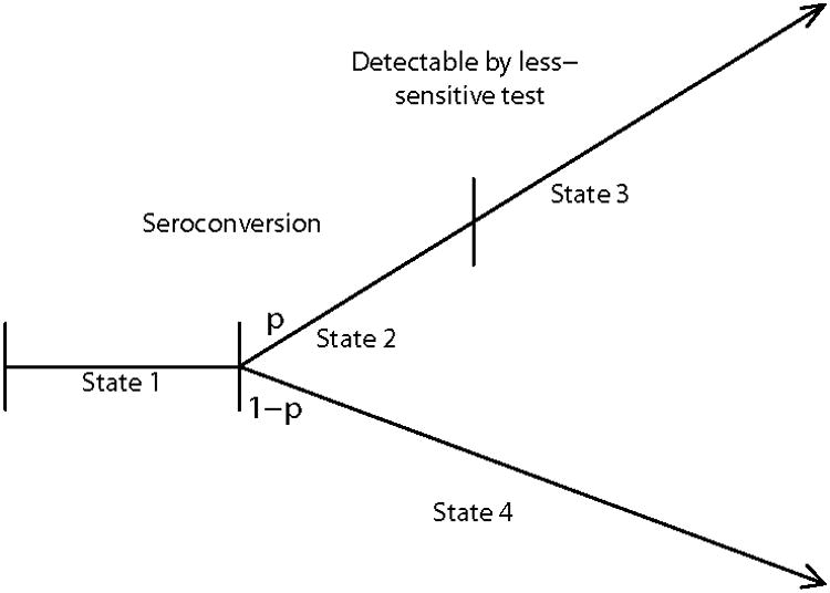
Four-State Model in which a Proportion, 1 − p, of Infected Persons Would Indefinitely Remain Non-Reactive to the Less-Sensitive Test

Suppose subpopulation membership is independent of the risk of infection and subsequent HIV progression, and that the incidence density is constant for a period of time preceding the cross-sectional sample. Then (Appendix 4) the maximum likelihood estimator of I for the model in Figure 2 is

$${\widehat{ℐ}}_p=\frac{p{N}_2-(1-p)N_3}{p{N}_1\mu },$$ (9)

provided the numerator is nonnegative, and zero otherwise. Note that this estimator reduces to the unadjusted estimator in (1) when p = 1. The estimator in (9) also arises using a mathematical modeling approach for estimating incidence developed by McWalter and Welte.⁷ Recognition that the McWalter-Welte estimator is also the maximum likelihood estimator of I for the model in Figure 2 ensures that, as the cross-sectional sample size becomes large, it will converge to the true incidence rate and be the most efficient (smallest variance) cross-sectional estimator for this setting.

In practice, p is not known exactly, and thus the estimator used in practice is (9) with p replaced by an estimator, say p̂; that is,

$${\widehat{I}}_p=\frac{\widehat{p}{N}_2-(1-\widehat{p})N_3}{\widehat{p}{N}_1\mu },$$ (10)

provided the numerator is nonnegative, and zero otherwise. Estimates of the variance of (9) and (10) are given in Appendix 4, and can be used to form confidence intervals for I. Methods for estimating p are considered in the DISCUSSION.

When p < 1, it is easily verified from Appendix 1 that

$$\text{sens}-{\text{spec}}_1\ge 1-p>0$$

for p < 1. Therefore, the assumption made by Hargrove et al that sens − spec₁ = 0 cannot hold for the model in Figure 2 with p < 1.

To illustrate the relative performance of the adjusted estimators of HIV incidence for the model in Figure 2, we conducted a simulation study using the same settings as in the previous simulation study, except that now a proportion 1 − p = 3%, 5%, or 7% of the population never become reactive on the less-sensitive test. Full results are available upon request. The results for a 10% prevalence and μ = 0.5 are summarized in Table 2. Consistent with the theoretical results, the McDougal adjusted and maximum likelihood estimators are essentially unbiased, with the McDougal adjusted estimators being less precise than maximum likelihood estimator.

Table 2.

Comparison of Adjusted Estimators of HIV Incidence Rate for Model in Figure 2 ¹.

		p = .93		p = .95		p = .97
Incidence Rate	Estimator (eq. #)	Expected Value2	Standard Error2	Expected Value2	Standard Error2	Expected Value2	Standard Error2
2%	Max. Likelihood
	known p (9)	2.0%	0.50%	2.0%	0.49%	2.0%	0.45%
	estd.3 p (10)	2.0%	0.66%	2.0%	0.64%	2.0%	0.56%
	Adjusted
	known sens/spec (2)	2.0%	0.75%	2.0%	0.73%	2.0%	0.68%
	estd.3 sens/spec (7)	2.0%	0.98%	2.0%	0.97%	2.0%	0.92%
	known sens/spec1/spec2 (4)	2.0%	0.56%	2.0%	0.54%	2.0%	0.50%
	estd.3 sens/spec1/spec2 (8)	2.0%	0.70%	2.0%	0.68%	2.0%	0.62%
4%	Max. Likelihood
	known p (9)	4.0%	0.64%	4.0%	0.61%	4.0%	0.59%
	estd.3 p (10)	4.0%	0.75%	4.0%	0.71%	4.0%	0.65%
	Adjusted
	known sens/spec (2)	4.0%	0.99%	4.0%	0.95%	4.0%	0.91%
	estd.3 sens/spec (7)	3.9%	1.23%	4.0%	1.16%	4.0%	1.12%
	known sens/spec1/spec2 (4)	4.0%	0.73%	4.0%	0.69%	4.0%	0.67%
	estd.3 sens/spec1/spec2 (8)	4.0%	0.81%	4.0%	0.78%	4.0%	0.75%
8%	Max. Likelihood
	known p (9)	8.0%	0.83%	8.0%	0.81%	8.0%	0.81%
	estd.3 p (10)	8.0%	0.89%	8.0%	0.85%	8.0%	0.83%
	Adjusted
	known sens/spec (2)	8.0%	1.42%	8.0%	1.39%	8.0%	1.37%
	estd.3 sens/spec (7)	7.9%	1.59%	8.0%	1.55%	8.0%	1.54%
	known sens/spec1/spec2 (4)	8.1%	1.06%	8.1%	1.04%	8.1%	1.03%
	estd.3 sens/spec1/spec2 (8)	8.1%	1.14%	8.1%	1.10%	8.1%	1.10%

¹Based on a cross-sectional sample of size N = 3000 from a population with 10% prevalence and window period with mean of 0.5 years and standard deviation of 0.6 years.

²Estimated by 2000 simulated studies. Estimated incidence taken to be 0 for simulations in which numerator of adjusted estimator is negative.

³Estimated sensitivity, specificity and p are drawn from a normal distribution with standard errors of 2%, symmetrically truncated with an upper limit of 1, as in Table 1.

Robustness of Estimators to the Assumed Model

The previous sections indicate that the optimal incidence estimator depends on whether or not all infected subjects become reactive to the less-sensitive test. Below we indicate how both the adjusted and unadjusted estimators of incidence can be biased when the wrong underlying model is assumed.

Suppose first that the unadjusted estimator is used, but that the correct model is that shown in Figure 2, for some p < 1. This might occur when the longitudinal study used to approximate μ and p had relatively few serconverters, all of whom subsequently became reactive to the less-sensitive test, thus resulting in an accurate estimate of μ but an estimated p of 1. For example, with p = .97 and 20 seroconverters, there is a 54% chance that none of the recent infections are from the subpopulation that will indefinitely remain non-reactive to the less-sensitive test.

It is shown in Appendix 6 that the unadjusted estimator (1) in this setting converges to

$$\mathit{\text{pI}}+\frac{(1-p)(1-\varphi )}{\varphi \mu },$$ (11)

as N gets large, where 1 − φ is the HIV prevalence rate at the time of the cross-sectional sample. The constraint that the prevalence in state 2 is less than the overall infection prevalence implies that I < (1 − φ)/(φμ), which in turn ensures that this limit must always exceeds the true incidence I. For example, when p = 95%, μ = 0.5 years, the prevalence is 10%, and the true incidence rate is 2%, 4%, and 10%, the unadjusted estimator will actually converge to 3.01%, 4.91%, and 10.6%, respectively.

Next suppose that the estimator (9) is used with some values, say p₀ and μ₀, for p and μ, but that in fact the model in Figure 1 holds. This might arise because the longitudinal study used to approximate μ and p did not follow infected subjects for sufficient time, resulting in some not yet becoming reactive to the less-sensitive test, and hence leading to underestimating μ by μ₀ and p (= 1) by p₀ < 1. It is shown in Appendix 6 that the adjusted estimator in (9) converges to

$$\frac{\mu }{{\mu }_0{p}_0}I-\frac{(1-p_0)(1-\varphi )}{\varphi {\mu }_0{p}_0}.$$ (12)

The adjusted estimator will thus be biased in this setting, and could either underestimate or overestimate the true incidence I. To illustrate using an example suggested by a referee, suppose that p = 1 and L has an exponential distribution with mean μ = 1, and that the cohort study used to approximate p and μ only followed subjects for 3 years. This would, on average, lead to p₀ = .95 and μ₀ = 0.95. With a prevalence of 10% (φ = 0.9) and true incidence rates of 2%, 4%, and 8%, the adjusted incidence estimator (9) will converge to 1.60%, 3.82%, and 8.25%, respectively.

Discussion

When every infected individual would eventually become reactive to the less-sensitive test (Figure 1), the unadjusted cross-sectional incidence estimator (equation 1) will always be more precise than the adjusted incidence estimators, and does not require external estimates of sensitivity and specificity parameters. On the other hand, when the less-sensitive test would never become reactive in a subset of the population (Figure 2), the most efficient estimation of incidence is given by the maximum likelihood estimator (9), which coincides with the estimator developed by McWalter and Welte⁷ using mathematical models. This estimator requires an external estimate of the size of this subpopulation, and the precision of this external estimate needs to be accounted for to obtain valid confidence intervals for the underlying incidence rate I.

When the assumptions about the underlying model (Figure 1 versus Figure 2) is wrong, both the unadjusted and adjusted incidence estimators can be biased. Thus, a key issue is how to determine which model reflects the practical setting under consideration. Since the model in Figure 1 is the special case of the model in Figure 2 corresponding to p = 1, determining the correct model can be viewed as accurately estimating p. Estimation of sens, spec, spec₁, and spec₂ typically relies on external information from longitudinal studies that identify time of seroconversion with reasonable accuracy; such studies are relatively hard to conduct. In contrast, estimation of p can be achieved by an appropriate external cross-sectional sample of subjects known to have been infected for longer than L_max, the maximum possible time from seroconversion until reactivity with the less-sensitive test among infected subjects that eventually become reactive (McWalter and Welte, unpublished manuscript). Although stored samples from individuals who have been infected for long periods are abundant, obtaining an appropriate external sample is challenging because the sample must representative of the population from which the cross-sectional sample (N₁, N₂, N₃) is obtained and, as a referee pointed out, this requires knowledge of L_max, which is not well characterized for a variety of experimental settings. For the BED capture enzyme immunoassay, Barnighausen et al¹⁶ examine the stability of estimates of 1 − p for possible values of L_max varying from 250 to 400 days, using nested samples of subjects obtained from a surveillance study in South Africa. Their results show no evidence of a decreasing rate of non-reactive subjects, suggesting that L_max may be smaller than these candidate values. An alternative approach is to initially estimate the proportion of non-reactive subjects from a random sample known to be infected for more than a candidate value of L_max, say 1 year, and to then test samples from the non-reactive subjects at later times (say, .5, 1, and 1.5 years later) to see if they remain non-reactive. Decreasing numbers of non-reactive samples would be evidence that a larger assumed value of L_max is needed. Another approach is to test independent samples of subjects known to have been infected for differing time periods (say, 1, 1.5, 2, and 2.5 years), and assess the stability of the proportions who are non-reactive.

We have assumed that the cross-sectional sample was drawn from an apparently healthy (asymptomatic) population. Biased incidence estimates can result from a sample drawn from a more general population that includes persons with late-stage HIV infection because of their increased risk of death¹³ and because some of these individuals may previously have been reactive to the less-sensitive assay but became non-reactive with advancing HIV infection. For such samples, valid estimates of incidence can be obtained when based only on asymptomatic individuals¹³.

Use of antiretroviral treatments (ARTs) by individuals in the cross-sectional sample also can bias incidence estimates because ARTs suppress assay SOD levels, and thus can make a previously reactive individual non-reactive to the less-sensitive assay. Currently, ART initiation occurs several years following seroconversion, typically more than L_max time units. In such settings, the unadjusted estimator based on the model in Figure 1 will remain valid if all sampled individuals taking ARTs are regarded as being in State 3, regardless of their reactivity to the less-sensitive test. However, appropriate modification of the adjusted estimates of incidence based on the model in Figure 2 is more complicated because the impact of ARTs on SOD levels might be different in the 2 subpopulations. ART use that occurs relative soon following seroconversion and unrecognized ART use among the N sampled subjects further complicates the estimation of incidence. More research in this area is needed.

Throughout this paper we have assumed that the cross-sectional sample was a random sample from the population of interest. The importance of a random sample cannot be overemphasized, as use of a “convenience” or other non-random sample can distort results in ways that are usually impossible to quantify. We also have assumed that the mean window period μ is known. However, when using cross-sectional methods to estimate incidence an estimate of μ must be used. When a biased estimate of μ is used, all estimators of HIV incidence discussed in this paper would, in general, be biased. This underscores the need for carefully conducted and analyzed longitudinal cohort studies to estimate μ for different less-sensitive tests, as well as the identification of virologic, demographic, and other factors that might affect μ.^1,3,4,5,6 An alternative to the standard approach of using an external estimator of μ is to employ an augmented cross-sectional design in which the subset of subjects found to be in the recent-infection state are followed forward in time for reactivity to the less-sensitive test; Wang and Lagakos (unpublished manuscript) demonstrate how this can be used to obtain internal estimators of the mean window period and proportion, 1 − p, of the population that woulud never become reactive to the less-sensitive test.

Appendices.

In what follows, we make the assumptions used in Balasubramanian and Lagakos¹³ for the model in Figure 1; namely, that time in State 2 is independent of time in State 1, and that the density function, f(u), for HIV infection is constant, say f(u) = f, for a period L_max prior to the time, t, at which the cross-sectional sample is drawn. In this interval, f = φI, where 1 − φ is the prevalence at time t. We let E + (E−) denote that the ELISA is reactive (non-reactive), and let LS + (LS−) denote that the less-sensitive tests is reactive (non-reactive), and let G(x) denote the cumulative distribution function of time in State 2.

Appendix 1.

Expressions for sens, spec, spec₁, and spec₂ for Model in Figure 1

For a individual found to be infected, let Y denote the elapsed time from seroconversion until the time of the test. Let L_max denote the upper limit of support for L. For any constants a, b satisfying 0 ≤ a < b < L_max,

$$P[\mathit{\text{LS}}-|E+,Y\in (a,b)]=\frac{P[E+,\mathit{\text{LS}}-,Y\in (a,b)]}{P[E+,Y\in (a,b)]}=(A)/(B).$$

Note that

$$(A)={\int }_{t-b}^{t-a}f(\nu )[1-G(t-\nu )]\mathit{\text{d}}\nu =f[(b-a)-{\int }_{t-b}^{t-a}G(t-\nu )\mathit{\text{d}}\nu ]=\varphi I[(b-a)-{\int }_a^{b}G(x)\mathit{\text{dx}}],$$

and

$$(B)=P[E+,Y\in (a,b)]={\int }_{t-n}^{t-a}f(\nu )\mathit{\text{d}}\nu =f(b-a)=\varphi I\mu .$$

Combining these,

$$P[\mathit{\text{LS}}-|E+,Y\in (a,b)]=1-\frac{1}{b-a}{\int }_a^{b}G(x)\mathit{\text{dx}}\text{for}b\le L_{max}$$ (A.1)

Using similar arguments when b > L_max, we get

$$P[\mathit{\text{LS}}-|E+,Y\in (a,b)]=\frac{f(L_{max}-a)-f{\int }_a^{L_{max}}G(x)\mathit{\text{dx}}}{1-\varphi -a\varphi I-F(t-b)}\text{for}b\ge L_{max}$$ (A.2)

An expression for sens is obtained by setting a = 0 and B = μ in (A.1), yielding

$$\text{sens}=1-\frac{1}{\mu }{\int }_0^{\mu }G(x)\mathit{\text{dx}},$$ (A.3)

and 1-spec is obtained by setting a = μ and b = ∞ in (A2), yielding

$$\text{spec}=1-\frac{\varphi I{\int }_0^{\mu }G(x)\mathit{\text{dx}}}{1-\varphi -\varphi I\mu }.$$ (A.4)

Using (A.1) with a = μ and b = 2μ gives 1-spec₁, and using (A.2) with a = 2μ and b = ∞ gives 1-spec₂. This yields

$${\text{spec}}_1=\frac{{\int }_{\mu }^{2\mu }G(x)\mathit{\text{dx}}}{\mu },$$ (A.5)

and

$${\text{spec}}_2=\frac{1-\varphi -\varphi I\mu -\varphi I{\int }_0^{2\mu }G(x)\mathit{\text{dx}}}{1-\varphi -2\varphi I\mu }.$$ (A.6)

It is easily verified that the overall specificity is related to spec₁ and spec₂ by

$$\text{spec}=\pi {\text{spec}}_1+(1-\pi ){\text{spec}}_2,$$

where

$$\pi =\frac{\varphi I\mu }{1-\varphi -\varphi I\mu }=P(\mu <Y<2\mu |E+,Y>\mu ).$$

Appendix 2.

Expectation and Convergence of Ñ_2L and N̂_2L; Convergence of ₁ and ₂ for Model in Figure 1

Substituting the expressions for sens and spec into (3), we have

$$E({\widehat{\mathcal{N}}}_{2L})=N\frac{I\varphi \mu -(1-\varphi )\frac{\varphi I{\int }_0^{\mu }G(x)\mathit{\text{dx}}}{1-\varphi -\varphi I\mu }}{1-\frac{1}{\mu }{\int }_0^{\mu }G(x)\mathit{\text{dx}}-\frac{\varphi I{\int }_0^{\mu }G(x)\mathit{\text{dx}}}{1-\varphi -\varphi I\mu }}=N\varphi I\mu \frac{1-(1-\varphi )\frac{1}{\mu }\frac{{\int }_0^{\mu }G(x)\mathit{\text{dx}}}{1-\varphi -\varphi I\mu }}{1-\frac{1}{\mu }{\int }_0^{\mu }G(x)\mathit{\text{dx}}-\frac{\varphi I{\int }_0^{\mu }G(x)\mathit{\text{dx}}}{1-\varphi -\varphi I\mu }}=N\varphi I\mu =E(N_2)$$

Rewrite (3) as

$${\widehat{\mathcal{N}}}_{2L}=\frac{N_2\text{spec}-N_3(1-\text{spec})}{\text{sens}+\text{spec}-1}.$$ (A.7)

Dividing the numerator and denominator of (2) by N and letting N → ∞, the probability limit of (2) is

$$\frac{\varphi I\mu -(1-\varphi )(1-\text{spec})}{(\text{sens}+\text{spec}-1)\varphi \mu }=\frac{I}{(\text{sens}+\text{spec}-1)}-\frac{(1-\varphi )(1-\text{spec})}{(\text{sens}+\text{spec}-1)\varphi \mu }.$$ (A.8)

Substituting the expressions for sens and spec into this limit to equal to I whenever spec< 1. When spec= 1, the limit also equals I when sens= 1.

Similarly,

$$E({\stackrel{\sim }{\mathcal{N}}}_{2L})=N\frac{\varphi I\mu -(1-\varphi )(1-{\text{spec}}_2)}{\text{sens}-{\text{spec}}_1+2{\text{spec}}_2-1}=N\frac{\varphi I\mu +(1-\varphi )({\text{spec}}_2-1)}{(\text{sens}-{\text{spec}}_1+2({\text{spec}}_2-1)+1)}=N\frac{\varphi I\mu (1+(1-\varphi )\frac{(1-\frac{1}{\mu }{\int }_0^{2\mu }G(x)\mathit{\text{dx}})}{1-\varphi -2\varphi I\mu }}{2-\frac{1}{\mu }{\int }_0^{2\mu }G(x)\mathit{\text{dx}}+2\varphi I\mu \frac{(1-\frac{1}{\mu }{\int }_0^{2\mu }G(x)\mathit{\text{dx}})}{1-\varphi -2\varphi I\mu }}=N\frac{\varphi I\mu (1+(1-\varphi )\frac{(1-\frac{1}{\mu }{\int }_0^{2\mu }G(x)\mathit{\text{dx}})}{1-\varphi -2\varphi I\mu })}{(1+(1-\varphi )\frac{(1-\frac{1}{\mu }{\int }_0^{2\mu }G(x)\mathit{\text{dx}})}{1-\varphi -2\varphi I\mu })}=N\varphi I\mu =E(N_2)$$

Dividing the numerator and denominator of (4) by N and letting N → ∞, it follows that the probability limit of ₂ is I.

Appendix 3.

Proof that Var( ₁) > Var(Î) and Var( ₂) > Var(Î) for Model in Figure 1

From (A.7),

$$\begin{array}{l}\mathit{\text{Var}}({\widehat{ℐ}}_1)=\mathit{\text{Var}}(\frac{N_2}{N_1\mu })\frac{{\text{spec}}^2}{{(\text{sens}+\text{spec}-1)}^2}+\mathit{\text{Var}}(\frac{N_3}{N_1\mu })\frac{{(1-\text{spec})}^2}{{(\text{sens}+\text{spec}-1)}^2}-2\mathit{\text{Cov}}(\frac{N_2}{N_1\mu },\frac{N_3}{N_1\mu })\frac{\text{spec}(1-\text{spec})}{{(\text{sens}+\text{spec}-1)}^2}\\ =\mathit{\text{Var}}(\widehat{I})\frac{{\text{spec}}^2}{{(\text{sens}+\text{spec}-1)}^2}+\mathit{\text{Var}}(\frac{N_3}{N_1\mu })\frac{{(1-\text{spec})}^2}{{(\text{sens}+\text{spec}-1)}^2}-2\mathit{\text{Cov}}(\frac{N_2}{N_1\mu },\frac{N_3}{N_1\mu })\frac{\text{spec}(1-\text{spec})}{{(\text{sens}+\text{spec}-1)}^2}>\mathit{\text{Var}}(\widehat{I}),\end{array}$$

where the last inequality holds because

$${\text{spec}}^2>{(\text{sens}+\text{spec}-1)}^2,\mathit{\text{Var}}(\frac{N_3}{N_1\mu })\frac{{(1-\text{spec})}^2}{{(\text{sens}+\text{spec}-1)}^2}>0,\text{and}\mathit{\text{Cov}}(\frac{N_2}{N_1\mu },\frac{N_3}{N_1\mu })<0.$$

The same approach yield Var( ₂) > Var(Î) by showing that ${\text{spec}}_2^2>{(\text{sens}-{\text{spec}}_1+2{\text{spec}}_2-1)}^2$. This can be verified by substituting (A.3), (A.5), and (A.6) into this expression and simplifying.

Appendix 4.

Maximum Likelihood Estimator of HIV Incidence Rate for Model in Figure 2

The likelihood function for (I, φ) based on (N₁, N₂, N₃) can be written as:

$$L(\varphi ,I,n_1)={\varphi }^{N_1}{[\varphi Ip\mu +(1-p)(1-\varphi )]}^{N_2}{\{p[1-\varphi -\varphi I\mu ]\}}^{N_3}.$$ (A.9)

From (A.9), the log of the likelihood is

$$\ell (\varphi ,I)\propto N_1\text{log}(\varphi )+N_2\text{log}[\varphi \mathit{\text{Ip}}\mu +(1-p)(1-\varphi )]+N_3\text{log}(1-\varphi -\varphi I\mu ),$$

from which one obtains the partial derivatives

$$\frac{\partial \ell }{\partial I}=\frac{N_2\varphi p\mu }{\varphi \mathit{\text{Ip}}\mu +(1-p)(1-\varphi )}-\frac{N_3\mu \varphi }{1-\varphi -\varphi I\mu },\text{and}\frac{\partial \ell }{\partial \varphi }=\frac{N_1}{\varphi }+\frac{N_2(\mathit{\text{Ip}}\mu -(1-p))}{\varphi \mathit{\text{Ip}}\mu +(1-p)(1-\varphi )}-\frac{N_3(1+I\mu )}{1-\varphi -\varphi I\mu }.$$

Setting these to zero and solving gives maximum likelihood estimators:

$$\widehat{\varphi }=\frac{N_1}{N},\text{and}\widehat{I}=\frac{p{N}_2-(1-p)N_3}{p{N}_1\mu }.$$

The matrix of negative second derivatives of ℓ(φ, I) with φ and I replaced by their maximum likelihood estimates, can be shown to have (1,1), (1,2), and (2,2) elements $N_1^2{p}^2{\mu }^2(\frac{1}{N_2}+\frac{1}{N_3}),N_1\mathit{\text{Np}}\mu (\frac{1}{N_2}(\frac{\mathit{\text{pN}}-N_3}{N_1}-1)+\frac{1}{N_3}\frac{\mathit{\text{pN}}-N_3}{N_1})$, and $N^2(\frac{1}{N_1}+\frac{{(\frac{\mathit{\text{pN}}-N_3}{N_1}-1)}^2}{N_2}+\frac{{(\frac{\mathit{\text{pN}}-N_3}{N_1})}^2}{N_3})$. Estimated variances for Î and φ̂ are obtained as the diagonals of the inverse of this matrix. This gives

$$\widehat{\text{Var}}(\widehat{I_p})=\frac{N_2}{N_1^{2}p{\mu }^2},\text{and}\widehat{\text{Var}}(\widehat{\varphi })=\frac{N_1(N-N_1)}{N^3}.$$

Regularity conditions for the asymptotic properties of the maximum likelihood estimator hold.¹⁷

When p is estimated externally, note that (N₁, N₂, N₃) ∼ Multinomial(N; φ, p₂, p₃) where

$$p_2=p\varphi I\mu +(1-p)(1-\varphi )\text{and}{p}_3=p(1-\varphi -\varphi I\mu ).$$

We use the fact that

$$\mathit{\text{Var}}({\widehat{I}}_p)={\mathit{\text{Var}}}_{\widehat{p}}[E({\widehat{I}}_p|\widehat{p})]+E_{\widehat{p}}[\mathit{\text{Var}}({\widehat{I}}_p|\widehat{p})]=(A)+(B).$$

$$\begin{array}{l}\text{where}(A)={\mathit{\text{Var}}}_{\widehat{p}}[E(\frac{\widehat{p}{N}_2-(1-\widehat{p})N_3}{\widehat{p}{N}_1\mu }|\widehat{p})]\approx {\mathit{\text{Var}}}_{\widehat{p}}[\frac{\widehat{p}N{p}_2-(1-\widehat{p})N{p}_3}{\widehat{p}N\varphi \mu }]\\ ={\mathit{\text{Var}}}_{\widehat{p}}[\frac{p_3}{\widehat{p}\varphi \mu }]\approx \frac{p_3}{{\varphi }^2{\mu }^2{p}^4}\mathit{\text{Var}}(\widehat{p})\end{array}$$

$$\text{and}(B)\approx E_{\widehat{p}}[\frac{N_2}{N_1^2\widehat{p}{\mu }^2}]\approx \frac{N_2}{N_1^{2}p{\mu }^2}$$

Therefore,

$$\widehat{\mathit{\text{Var}}}({\widehat{I}}_p)=\frac{N_2}{N_1^2{\mu }^2\widehat{p}}+\frac{N_3^2}{N_1^2{\mu }^2{\widehat{p}}^4}\mathit{\text{Var}}(\widehat{p}).$$

Appendix 5.

Limit of Adjusted Estimators for Model in Figure 2

Under the 4-state model in Figure 2, the probability limits of N₂/N and N₁/N are φIpμ + (1 − p)(1 − φ) and φ respectively. Let sens*, spec*, ${\text{spec}}_1^{\ast }$ and ${\text{spec}}_2^{\ast }$ denote the algebraic expressions for sens, spec, spec₁, and spec₂ under the model in Figure 1, given in (A.3), (A.4), (A.5), and (A.6), respectively. It is easily verified that

$$\begin{array}{l}\text{sens}={\text{sens}}^{\ast }\cdot p+(1-p)\\ \text{spec}={\text{spec}}^{\ast }\cdot p\\ {\text{spec}}_1={\text{spec}}_1^{\ast }\cdot p\\ {\text{spec}}_2={\text{spec}}_2^{\ast }\cdot p\end{array}$$

Therefore,

$$\begin{array}{l}E({\widehat{\mathcal{N}}}_{2L})=N\frac{\varphi I\mu p+(1-p)(1-\varphi )-(1-\varphi )(1-{\text{spec}}^{\ast }\cdot p)}{{\text{sens}}^{\ast }\cdot p+(1-p)+{\text{spec}}^{\ast }\cdot p-1}\\ =N\frac{\varphi I\mu +(1-\varphi )({\text{spec}}^{\ast }-1)}{{\text{sens}}^{\ast }+{\text{spec}}^{\ast }-1}=N\varphi I\mu ,\end{array}$$

where the last step follows from Appendix 2.

Also,

$$\begin{array}{l}E({\stackrel{\sim }{N}}_{2L})=N\frac{\varphi I\mu p+(1-p)(1-\varphi )-(1-\varphi )(1-{\text{spec}}_2^{\ast }\cdot p)}{{\text{sens}}^{\ast }\cdot p+(1-p)-{\text{spec}}_1^{\ast }\cdot p+2({\text{spec}}_2^{\ast }\cdot p)-1}\\ =N\frac{\varphi I\mu p+(1-p)(1-\varphi )-(1-\varphi )(1-p+p-{\text{spec}}_2^{\ast }\cdot p)}{({\text{sens}}^{\ast }-{\text{spec}}_1^{\ast }+2{\text{spec}}_2^{\ast }-1)p}\\ =N\frac{(\varphi I\mu +(1-\varphi )({\text{spec}}_2^{\ast }-1))\cdot p}{({\text{sens}}^{\ast }-{\text{spec}}_1^{\ast }+2{\text{spec}}_2^{\ast }-1)p}\\ =N\frac{(\varphi I\mu +(1-\varphi )({\text{spec}}_2^{\ast }-1))}{({\text{sens}}^{\ast }-{\text{spec}}_1^{\ast }+2{\text{spec}}_2^{\ast }-1)}\\ =N\varphi I\mu ,\end{array}$$

where the last step follows from Appendix 2. Using similar arguments, the probability limit of ₂equals I.

Note that although McDougal et al⁵ allude to the assumption that L_max is less than 2μ, the McDougal adjusted formula ₂ remains valid regardless of whether this assumption holds or not. Also, under the setting where L_max < 2μ, it can be verified that sens − spec₁ = 1 − p and spec₂ = p. Using these relations, it is easily verified that ₂ reduces to the unadjusted estimator Î for the model in Figure 1, and to the maximum likelihood estimator _p for the model in Figure 2.

Appendix 6.

Limits of Unadjusted and Maximum Likelihood Estimators when Assumed Model does not Hold

Under the 4-state model in Figure 2, the probability limits of N₂/N and N₁/N are φIpμ + (1 − p)(1 − φ) and φ respectively. The probability limit of the unadjusted estimator is therefore

$$\frac{\varphi Ip\mu +(1-p)(1-\varphi )}{\varphi \mu }=pI+\frac{(1-p)(1-\varphi )}{\varphi \mu }.$$

Now suppose the model in Figure 1 holds, and that the cohort study used to estimate p and μ only follows subjects until time τ < L_max, and incorrectly assumes that any infected person that has not yet become reactive on the less-sensitive test will never become reactive. Let μ₀ and p₀ denote the expectations of the resulting (under) estimates of μ and p, respectively; that is, μ₀ = E(L|L <= τ), and p₀ = G(τ). Then as the size of the cross-sectional sample grows large, the adjusted estimator (9) converges in probability to

$$\begin{array}{l}{\widehat{I}}_p=\frac{{\widehat{p}}_0{N}_2-(1-{\widehat{p}}_0)N_3}{{\widehat{p}}_0{N}_1{\widehat{\mu }}_0}\\ \to \frac{p_0\varphi I\mu N-(1-p_0)((1-\varphi -\varphi I\mu )N)}{p_0(\varphi N){\mu }_0}\\ =\frac{\mu }{{\mu }_0{p}_0}I-\frac{(1-\varphi )(1-p_0)}{\varphi {\mu }_0{p}_0}.\end{array}$$

References

- 1.Lagakos SW, Gable A, editors. Methodological Challenges in HIV Biomedical Prevention Trials. Washington: Institute of Medicine, National Academy Press; 2008. [Google Scholar]
- 2.Janssen RS, Satten GA, Stramer SL, Rawal BD, O'Brien TR, Weiblen BJ, et al. New Testing Strategy to Detect Early HIV-1 Infection for Use in Incidence Estimates and for Clinical and Prevention Purposes. JAMA. 1998;280:42–48. doi: 10.1001/jama.280.1.42. [DOI] [PubMed] [Google Scholar]
- 3.Karita E, Price M, Hunter E, Chomba E, Allen S, Fei L, et al. Investigating the Utility of the HIV-1 BED Capture Enzyme Immunoassay Using Cross-Sectional and Longitudinal Seroconverter Specimens from Africa. AIDS. 2007;21:403–408. doi: 10.1097/QAD.0b013e32801481b7. [DOI] [PubMed] [Google Scholar]
- 4.Sakarovitch C, Rouet F, Murphy G, Minga AK, Alioum A, Dabis F, et al. Do Tests Devised to Detect Recent HIV-1 Infection Provide Reliable Estimates of Incidence in Africa? J Acquir Immune Defic Syndr. 2007;45:115–122. doi: 10.1097/QAI.0b013e318050d277. [DOI] [PubMed] [Google Scholar]
- 5.McDougal JS, Parekh BS, Peterson ML, Branson BM, Dobbs T, Ackers M, et al. Comparison of HIV Type I Incidence Observed During Longitudinal Follow-Up with Incidence Estimated by Cross-Sectional Analysis Using the BED Capture Enzyme Immunoassay. AIDS Res Hum Retroviruses. 2006;22:945–952. doi: 10.1089/aid.2006.22.945. [DOI] [PubMed] [Google Scholar]
- 6.Hargrove JW, Humphrey JH, Mutasa K, Parekh BS, McDougal JS, Ntozinie R, et al. Improved HIV-1 Incidence Estimates Using the BED Capture Enzyme Immunoassay. AIDS. 2007;22:511–518. doi: 10.1097/QAD.0b013e3282f2a960. [DOI] [PubMed] [Google Scholar]
- 7.McWalter TA, Welte A. Relating Recent Infection Prevalence to Incidence with a Sub-Population of Non-Progressors. J Math Biol. 2009 doi: 10.1007/s00285-009-0282-7. in press. [DOI] [PubMed] [Google Scholar]
- 8.Welte A, McWalter TA, Bärnighausen T. A Simplified Formula for Inferring HIV Incidence from Cross-Sectional Surveys Using a Test for Recent Infection. AIDS Res Hum Retroviruses. 2009;25:125–126. doi: 10.1089/aid.2008.0150. [DOI] [PMC free article] [PubMed] [Google Scholar]
- 9.Brookmeyer R. Should Biomarker Estimates of HIV Incidence Be Adjusted? AIDS. 2009;23:485–491. doi: 10.1097/QAD.0b013e3283269e28. [DOI] [PubMed] [Google Scholar]
- 10.Constantine NT, Sill AM, Jack N, Kreisel K, Edwards J, Cafarella T, et al. Improved Classification of Recent HIV-1 Infection by Employing a Two-Stage Sensitive/Less-sensitive Test Strategy. J Acquir Immune Defic Syndr. 2004;32:94–103. doi: 10.1097/00126334-200301010-00014. [DOI] [PubMed] [Google Scholar]
- 11.Parekh BS, Kennedy MS, Dobbs T, Pau C, Byers R, Green T, et al. Quantitative Detection of Increasing HIV Type 1 Antibodies After Seroconversion: A Simple Assay for Detecting Recent HIV Infection and Estimating Incidence. AIDS Res Hum Retroviruses. 2002;18:295–307. doi: 10.1089/088922202753472874. [DOI] [PubMed] [Google Scholar]
- 12.Kaplan EH, Brookmeyer R. Snapshot Estimators of Recent HIV Incidence Rates. Operations Research. 1995;47:29–37. [Google Scholar]
- 13.Brookmeyer R, Quinn TC. Estimation of Current Human Immunodeficiency Virus Incidence Rates from a Cross-Sectional Survey Using Early Diagnostic Tests. Am J Epidemiology. 1995;141:166–172. doi: 10.1093/oxfordjournals.aje.a117404. [DOI] [PubMed] [Google Scholar]
- 14.Balasubramanian R, Lagakos SW. Estimating HIV Incidence Based on Combined Prevalence Testing. Biometrics. 2009 Apr 13; doi: 10.1111/j.1541-0420.2009.01242.x. Epub ahead of print. [DOI] [PMC free article] [PubMed] [Google Scholar]
- 15.Novitsky V, Wang R, Kebaabetswe L, Greenwald J, Rossenkhan R, Moyo S, Musonda R, Woldegabriel E, Lagakos SW, Essex M. Better Control of Early Viral Replication Is Associated with Slower Rate of Elicited Antiviral Antibodies in the Detuned EIA during Primary HIV-1 C Infection. J Acquir Immune Defic Syndr. 2009 Jun 11; doi: 10.1097/QAI.0b013e3181ab6ef0. Epub ahead of print. [DOI] [PMC free article] [PubMed] [Google Scholar]
- 16.Barninghausen T, Wallrauch C, Welte A, McWalter TA, Mbizana N, Viljoen J, Graham N, Tanser F, Puren A, Newell M-L. HIV Incidence in Rural South Africa: Comparison of Estimates from Longitudinal Surveillance and Cross-Sectional cBED Assay Testing. PLoS One. 2008;3:1–8. doi: 10.1371/journal.pone.0003640. [DOI] [PMC free article] [PubMed] [Google Scholar]
- 17.Cox D, Hinkley D. Theoretical Statistics. London: Chapman and Hall; 1974. [Google Scholar]