Automatic Image Analysis of Histopathology Specimens Using Concave Vertex Graph

Abstract

Automatic image analysis of histopathology specimens would help the early detection of blood cancer. The first step for automatic image analysis is segmentation. However, touching cells bring the difficulty for traditional segmentation algorithms. In this paper, we propose a novel algorithm which can reliably handle touching cells segmentation. Robust estimation and color active contour models are used to delineate the outer boundary. Concave points on the boundary and inner edges are automatically detected. A concave vertex graph is constructed from these points and edges. By minimizing a cost function based on morphological characteristics, we recursively calculate the optimal path in the graph to separate the touching cells. The algorithm is computationally efficient and has been tested on two large clinical dataset which contain 207 images and 3898 images respectively. Our algorithm provides better results than other studies reported in the recent literature.

1 Introduction

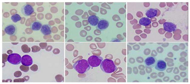
As new therapies emerge for blood cancer screening, it becomes increasingly important to distinguish among subclasses of lymphocytes in advance. Processing the specimen using a reliable, image-based analysis system could reduce the cost and patient morbidity. In image-based analysis the first step is segmentation. However, the traditional methods usually fail to accurately segment touching cells in the digitized hematologic specimens. Touching cells are especially prominent in malignant cases. In Figure 1, we show representative morphologies for benign and five hematologic malignancies (hematoxylin-eosin staining): Chronic Lymphocytic Leukemia (CLL) [1], Mantle Cell Lymphoma, (MCL) [2], Follicular Center Cell Lymphoma (FCC) [3], Acute Myelocytic Leukemia (AML) and Acute Lymphocytic Leukemia (ALL) [2].

Fig. 1.

Some representative morphologies of touching lymphocytes. In the first row, from left to right: CLL, MCL and FCC. In the second row, from left to right: ALL, AML and benign. The specimens were prepared at different hospitals and institutions therefore there exists large variations in staining.

The watershed algorithm is the most commonly used method for performing touching object segmentation. However, it suffers from several major drawbacks.

• Oversegmentation. The algorithm is sensitive to noise and often produces many oversegmented small regions. Marker-based watershed [4] can partially remedy this issue, but it requires manual selection or accurate estimation of the markers.

• Lack of shape prior. It is generally difficult to include shape priors in the watershed transform. Although there are some efforts [5,6] proposed for specific cases, the general problem still exists.

In this paper, we propose a novel algorithm to separate touching cells. The algorithm starts from a deformable model which extracts the boundary contour of the touching cells. The concave vertex graph is constructed using the concave vertices on the contour and the edges detected in the region of touching cells. The segmentation is then treated as an optimal grouping of pixels, which can be solved by recursively searching optimal shortest path in the concave vertex graph.

2 Boundary Contour Extraction

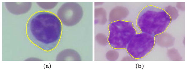
The initial step of the algorithm is to extract the boundary contour of the touching cells. We first apply a L₂E robust estimation [7] to provide a rough estimation of the outer boundaries of the cells inside the region of interest (ROI). A robust gradient vector flow (GVF) snake [8] using Luv [9, Sec. 8.4] color gradients is further applied to extract the objects from the background. Since the deformable models are initialized using the results of robust estimation, the convergence speed is increased and the method can handle topological changes. In this paper, we focus our attention on the touching cases shown in Figure 2b, where the output contour represents the outer boundary of the touching cells.

Fig. 2.

The segmentation result of robust color GVF snake. (a) The ROI contains only one cell. (b) The ROI contains the touching cells.

3 Concave Points and Inner Edges Detection

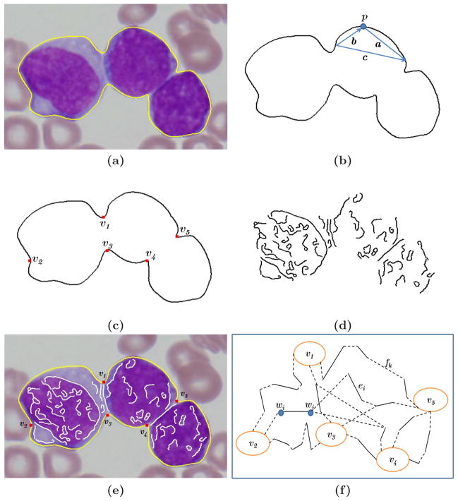
In Figure 3, we show the construction of the concave vertex graph. The contour found by boundary contour extraction algorithm is shown in Figure 3a. We detect the high curvature points on the contour via [10](Figure 3b). At each point p on the contour a set of triangles are constructed. The points which satisfy

Fig. 3.

Construction of the concave vertex graph. (a) The original image with the yellow boundary contour. (b) High curvature points detection. (c) Concave points detection. (d) Inner edges detection. (e) The outer boundary C, concave vertices V and inner edges E, superimposed on the original image. (f) The constructed concave vertex graph G. The filling edges are shown with dotted lines.

$$d_{min}\le \mid \mathit{a}\mid \le d_{max}{d}_{min}\le \mid \mathit{b}\mid \le d_{max}\alpha \le {\alpha }_{max}$$ (1)

where $\alpha =arccos\frac{{\mid \mathit{a}\mid }^2+{\mid \mathit{b}\mid }^2-{\mid \mathit{c}\mid }^2}{2\mid \mathit{a}\mid \mid \mathit{b}\mid }$ d_min, d_max = 7, 9 pixels and α_max = 150° are kept. The candidates are further processed to suppress the local nonmaxima points. The final high curvature points correspond to both concave and convex points. We keep only the concave points, shown as red rectangles in Figure 3c. This can be calculated from the sign of the cross product a ⊗ b, which has to be negative for concave points.

Canny edge detector is applied inside the cell region and straight line fitting is used to model the edges (Figure 3d). The separating curve combines a pair of convex vertices on the boundary and is enforced to pass through the inner edges.

4 Touching Cells Segmentation

The outer boundary of the touching cells is defined as C, and the region enclosed by C is R(C). The concave points are the set V, e.g. v1– v5 which are shown in Figure 3e. The inner edges are the set E, e.g. shown as white solid lines in Figure 3e and also illustrated by e_i in Figure 3f.

4.1 Concave Vertex Graph

In Figure 3f we construct the concave vertex graph G. Let W be the vertex set consisting of the end points of inner edges E, e.g. w_i and w_j in Figure 3f. The vertices of graph G are then equal to V ∪ W.

The graph has two sets of edges E and F. The set E contains the inner edges found by the edge detection algorithm. The set F is constructed with filling edges by connecting the vertices in G which are not connected by inner edges, e.g. f_k in Figure 3f. The lengths of the inner edges are set to ε (10⁻¹⁶), while the lengths of the filling edges in set F are given by the Euclidean distance between the two vertices of the edges.

The Dijkstra algorithm is used to find the shortest path p_ij between v_i and v_j. The length of the p_ij, ||p_ij ||, is given by the total length of the filling edges f_k in p_ij because the length of real inner edges is set to be ε

$$\Vert p_{ij}\Vert =\sum _{f_k\in p_{ij}}\mathit{length}(f_k).$$ (2)

In Figure 3f, as an example, we can see ||p₁₂|| > ||p₁₃|| because p₁₂ traverse longer filling edges than p₁₃. The defined path lengths enforce the segmentation to follow inner edges since the trivial solution to directly connect two concave vertices using only filling edges in graph G would provide a longer path.

Alg. 1.

The algorithm to separate touching cells using concave vertex graph

Input: Given the region of interest (ROI) containing touching cells. Extract the boundary contour C, detect the concave points V, the inner edges E in R(C), construct the concave vertex graph G. for each vertex v(i) ∈ V Find the path pij and calculate the length ||pij || using (2). Initialize mincost = +∞ and Q = Ø. while (V is not empty) for each vertex v(i) ∈ V * for each vertex v(j ≠ i) ∈ V Apply the path pij to separate the graph G in to L and R. Calculate the cost c using (6) and save in Q. Sort Q and pick up the path pij with the lowest cost c. if (c < 1.5 * mincost) Record path pij and the region R(C, pij) with cost c in the result. The edges and zero degree vertices in the R(C, pij) are removed from G. Set mincost = c and Q = Ø else return result.

After the Dijkstra algorithm is applied, we find all the shortest pathes among concave vertices, p_ij, which are valid candidates to separate touching cells. The key idea of our algorithm is to treat the touching cells segmentation as recursively searching for the best path p_ij in G, which minimizes a cost function specifically designed to prefer cell-like object-cut.

4.2 Cost Function

We are looking for perceptually “good” segmentation of touching cells. For this purpose, we design the cost function to represent the clues that surgical pathologists use for judgement.

• The cells should be objects which are perceptually salient, since humans intend to separate such objects in an image. A good definition of saliency is proposed in [11] based on the Gestalt laws [12]. We apply the minimum of two saliency costs

  $$c_s=min\left(\frac{\Vert p_{ij}\Vert }{\sqrt{{\mathit{area}}_L(C,p_{ij})}},\frac{\Vert p_{ij}\Vert }{\sqrt{{\mathit{area}}_R(C,p_{ij})}}\right)$$ (3)

  where ||p_ij|| is the length defined in (2), each path p_ij in G divides R(C) into two regions L and R, and the min function in (3) selects the region with the smallest cost. The area(C, p_ij) denotes the area enclosed by C and path p_ij.

• The cells are objects which are close to elliptical shape and can be modeled by ellipse fitting using points on C and p_ij. The ratio between the long and short axes is recorded as tg. The segmented objects are expected to provide a ratio tg in the range [tg₁, tg₂], in which case the dist (tg, [tg₁, tg₂]) = 0. Otherwise, we define dist (tg, [tg₁, tg₂]) = min (|tg − tg2|, |tg − tg1|).

  $$c_g=min\left(\frac{1}{1+exp(-\mathit{dist}({tg}_L,[{tg}_1,{tg}_2]))},\frac{1}{1+exp(-\mathit{dist}({tg}_R,[{tg}_1,{tg}_2]))}\right)$$ (4)

  where the L and R have the same definition as (3). The tg₁ and tg₂ represent the lower bound and upper bound of the long axes to short axes ratio.

• The cells are objects which have biologically reasonable areas. Following the definition above, we use ta₁ and ta₂ to represent the lower bound and upper bound of the cell area.

  $$c_a=min\left(\frac{1}{1+exp(-\mathit{dist}({ta}_L,[{ta}_1,{ta}_2]))},\frac{1}{1+exp(-\mathit{dist}({ta}_R,[{ta}_1,{ta}_2]))}\right).$$ (5)
• The final cost c is the weighted sum

  $$c={\lambda }_1{c}_s+{\lambda }_2{c}_g+{\lambda }_3{c}_a\sum _{i=1}^3{\lambda }_i=1.$$ (6)

  The optimal values of coefficients are selected as λ₁ = 0.5, λ₂ = 0.3 and λ₃ = 0.2, which are learned in an offline process using a training set and held constant throughout the experiments.

4.3 Algorithm

Using the concave vertex graph G and the cost function c, the method is described in Algorithm 1. It is recursively applied to separate touching cells until all the region R(C) are allocated to the segmented cells. The algorithm only separates the cytoplasm of the touching cells. Since the colors of nuclei and cytoplasm are distinct, they can be easily separated. In order to provide smooth boundaries, we apply the quadratic splines to postprocess the boundaries of each segmented cell.

5 Experiments

The cell database consists of a mixed set of 86 hematopathology cases: 18 Mantle Cell Lymphoma (MCL), 20 Chronic Lymphocytic Leukemia (CLL), 9 Follicular Center Cell Lymphoma (FCC), 18 Acute Lymphocytic Leukemia (ALL), 19 Acute Myelocytic Leukemia (AML), and 19 benign cases. For each case, there are varying number of cell images from 10 to 90. In total there exists 3898 cell images in our complete database. All the cases were generated from the archives of City of Hope Hospital in California, University of Pennsylvania of School of Medicine, Spectrum Health System, Grand Rapids, MI and Robert Wood Johnson Medical School, University of Medicine & Density of New Jersey.

The imaging platform for the experiments consisted of an Intel-based workstation interfaced with a high-resolution Olympus DP70 camera equipped with 12-bit color depth on each color channel and 1.45 million pixel effective resolution. The system also includes a single 2/3 inch CCD digital camera, an Olympus AX70 microscope equipped with a Prior 6-way robotic stage, motorized objective turret and a magnification changer.

We compare the segmentation results with manually segmentation. Two sets of experiments are performed.

• The 207 touching cases of the histopathology cell image dataset.

• The complete database which contains 3898 histopathology cell images.

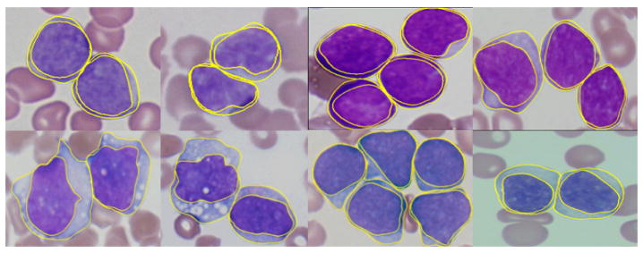
Figure 4 shows some segmentation results. In Table 1 we present the segmentation accuracies for the six different classes of lymphocytes in two set of experiments. We obtained an average accuracy 88.9% on the touching cells dataset and 90.1% on the complete database.

Fig. 4.

The segmentation results using the concave vertex graph

Table 1.

Segmentation accuracy(%) using the concave vertex graph. The accuracy_c and accuracy_n represent the segmentation accuracy for cytoplasm and nuclei respectively.

	Benign	CLL	MCL	FCC	AML	ALL
accuracyc (%) of touching cells	90.1	90.8	86.4	86.9	86.3	85.2
accuracyn (%) of touching cells	92.3	91.2	88.1	88.7	87.5	87.9
accuracyc (%) of all cells	92.5	91.7	87.2	89.1	88.5	87.6
accuracyn (%) of all cells	95.8	92.8	90.1	91.0	88.9	89.2

Only a limited number of recent literature addresses the issue of touching cells segmentation in histopathology images using hematoxylin staining in high resolution (60× in our case). The watershed algorithm [4] is widely accepted for touching object segmentation and successfully used in segmenting histopathology images [13]. We compared our method with watershed using the 207 touching cell image dataset and listed the results in Table 2. The 80% column in Table 2 represents the sorted 80% highest accuracy of all the results, and is commonly used by doctors to evaluate the usability of the system. The experiments demonstrate the superior performance of the presented approach.

Table 2.

The segmentation accuracy(%) using the watershed algorithm and the concave vertex graph

	Mean	Variance	Median	Min	Max	80%
Watershed	74.3	9.8	75.1	65.4	82.7	72.9
Concave Vertex Graph	88.9	5.1	90.2	75.2	95.5	87.1

6 Conclusion

In this paper, a novel segmentation algorithm has been proposed to address the challenges of touching cell segmentation in hematologic specimens. The results are validated using real clinical data containing six classes of hematologic blood cell images. We compare our algorithm with watershed and experimentally show the superior performance of the proposed algorithm.

For general pixel grouping problem using a normal graph, the optimization problem is N P -hard. Only certain cost function can be approximately solved using algorithm like normalized cut [14] in polynomial time. In our algorithm, the cost function is designed to meet the domain specific requirements. The concave vertex graph, which utilize the concave points of the outer contour, reduce the search space to the shortest pathes in the constructed graph G. Based on a MATLAB implementation, the algorithm can finish in less than 2 seconds for an 128×128 image.

References

- 1.Rozman C, Montserrat E. Chronic lymphocytic leukemia. The New England Journal of Medicine. 1995;333(16):1052–1057. doi: 10.1056/NEJM199510193331606. [DOI] [PubMed] [Google Scholar]
- 2.Cotran R, Kumar V, Collins T, Robbins S. Pathologic basis of disease. 5. W.B. Saunders Company; Philadelphia: 1994. [Google Scholar]
- 3.Aisenberg A. Coherent view of non-Hodgkin’s lymphoma. J Clin Oncol. 1995;13:2656–2675. doi: 10.1200/JCO.1995.13.10.2656. [DOI] [PubMed] [Google Scholar]
- 4.Moga AN, Gabbouj M. Parallel marker-based image segmentation with watershed transformation. Journal of Parallel and Distributed Computing. 1998;51(1):27–45. [Google Scholar]
- 5.Grau V, Mewes AUJ, Alcaniz M, Kikinis R, Warfield SK. Improved watershed transform for medical image segmentation using prior information. ITMI. 2004;23(4):447–458. doi: 10.1109/TMI.2004.824224. [DOI] [PubMed] [Google Scholar]
- 6.Nguyen HT, Ji Q. Improved watershed segmentation using water diffusion and local shape priors. CVPR. 2006;1:985–992. [Google Scholar]
- 7.Scott DW. Parametric statistical modeling by minimum integrated square error. Technometrics. 2001;43:274–285. [Google Scholar]
- 8.Yang L, Meer P, Foran D. Unsupervised segmentation based on robust estimation and color active contour models. IEEE Trans on Information Technology in Biomedicine. 2005;9:475–486. doi: 10.1109/titb.2005.847515. [DOI] [PubMed] [Google Scholar]
- 9.Wyszecki G, Stiles WS. Color Science: Concepts and Methods, Quantitative Data and Formulae. 2. Wiley; Chichester: 1982. [Google Scholar]
- 10.Chetverikov D, Szabó Z. A simple and efficient algorithm for detection of high curvature points in planar curves. The 23rd Workshop of the Austrian Pattern Recognition Group; 1999. pp. 175–184. [Google Scholar]
- 11.Stahl JS, Wang S. Convex grouping combining boundary and region information. ICCV. 2005;2:946–953. doi: 10.1109/tip.2007.904463. [DOI] [PubMed] [Google Scholar]
- 12.Elder JH, Goldberg RM. Ecological statistics of Gestalt laws for the perceptual organization of contours. Journal of Vision. 2002;2(4):324–353. doi: 10.1167/2.4.5. [DOI] [PubMed] [Google Scholar]
- 13.Adiga PSU, Chaudhuri BB. An efficient method based on watershed and rule-based merging for segmentation of 3D histo-pathological images. J Pattern Recognition. 2001;34(7):1449–1458. [Google Scholar]
- 14.Cai W, Chung AC. Multi-resolution vessel segmentation using normalized cuts in retinal images. In: Larsen R, Nielsen M, Sporring J, editors. MICCAI 2006. LNCS. Vol. 4191. Springer; Heidelberg: 2006. pp. 928–936. [DOI] [PubMed] [Google Scholar]