SNP Set Association Analysis for Familial Data

Abstract

Genome-wide association studies (GWAS) are a popular approach for identifying common genetic variants and epistatic effects associated with a disease phenotype. The traditional statistical analysis of such GWAS attempts to assess the association between each individual Single Nucleotide Polymorphism (SNP) and the observed phenotype. Recently, kernel machine-based tests for association between a SNP set (e.g., SNPs in a gene) and the disease phenotype have been proposed as a useful alternative to the traditional individual SNP approach, and allow for flexible modeling of the potentially complicated joint SNP effects in a SNP set while adjusting for covariates. We extend the kernel machine framework to accommodate related subjects from multiple independent families, and provide a score-based variance component test for assessing the association of a given SNP set with a continuous phenotype, while adjusting for additional covariates and accounting for within-family correlation. We illustrate the proposed method using simulation studies and an application to genetic data from the Genetic Epidemiology Network of Arteriopathy (GENOA) study.

1 Introduction

Genome-wide association studies (GWAS) have become a popular approach for identifying genetic variants that are related to disease risk or quantitative traits. Such studies are often performed in an initial discovery phase and involve genotyping hundreds of thousands of single nucleotide polymorphisms (SNPs) across a large number of subjects, and then searching for the specific variants that are associated with the outcome of interest. The standard approach for identifying association in unrelated subjects is to perform individual-SNP based analyses, typically involving a regression model of phenotype on individual genotype (possibly controlling for additional covariates) and resulting in a p-value for association for each SNP. Analyses of related subjects from family studies are often similarly analyzed on an individual SNP basis by incorporating a random effect in the regression model encapsulating the correlation of related subjects [e.g., Abecasis et al., 2000; Atkinson and Therneau, 2009]. Due to the large number of typed SNPs, the overall analysis is plagued with a substantial multiple testing burden, making it difficult for SNPs to reach genome-wide significance levels (e.g., p-values < 5 ×10⁻⁸). Consequently, individual-SNP based tests will tend to have limited power in identifying SNPs with small effects, which have been observed in many GWAS studies of complex traits [Manolio et al., 2009]. Many of the top SNPs are hence often false positives and cannot be replicated due to weak signals. Moreover, epistatic effects of SNPs (i.e., SNP-SNP interactions and joint effects) will fail to be detected in individual-SNP analysis.

Numerous multi-SNP or multi-marker tests have thus emerged as promising alternatives to individual-SNP analysis. Having selected a set of SNPs to be analyzed, e.g., based on genes, haplotype blocks, pathways, etc., one common approach for evaluating significance of the set of markers is to use methods based on individual SNP analysis and then adjust for multiple testing across multiple markers within the SNP set to control the false-positive rate [e.g., Moskvina and Schmidt, 2008; Gao et al., 2008; Conneely and Boehnke, 2007; Liu et al., 2010]. Omnibus or global tests in regression-type analysis for multiple markers avoid the problem of multiple testing within the set by testing all markers simultaneously [e.g., Schaid et al., 2002], but can be plagued by a large number of degrees of freedom [Wu et al., 2010, 2011]. A third class of methods attempts to address both of these issues by using notions of pairwise similarity [e.g., Wessel and Schork, 2006; Tzeng et al., 2009, 2011; Mukhopadhyay et al., 2010; Han and Pan, 2010]. The so-called ‘kernel-based’ methods of Kwee et al. [2008] and Wu et al. [2010] also fall into this class, as they rely on kernel functions that measure the pairwise similarity between subjects based on the genotypes of the SNPs within the set, and result in a single variance component test for each set. In a genome-wide setting, this type of analysis can improve power not only by reducing the number of hypotheses being tested, but also borrowing strength and information from correlated SNPs (i.e., SNPs in linkage disequilibrium (LD)) in the set by combining weak effects of individual SNPs for larger joint effects. The latter power gains will be realized when there are multiple SNPs in moderate to high LD with the causal variant(s). Thus, this approach is particularly appealing in situations where the true causal SNPs are not genotyped on a chip, but multiple typed SNPs in at least moderate LD with the true causal SNPs are available; hence the typed SNPs together can serve as a good surrogate for the untyped causal SNPs. The kernel machine models [Kwee et al., 2008; Wu et al., 2010] easily allow for adjustment of covariate effects, such as principal components to account for population stratification [Price et al., 2006], and flexible modeling of the functional relationship between SNPs in the set and outcome. Pan [2009] considered a similar SNP set test assuming linear SNP effects.

The aforementioned kernel-based methods are applicable to studies of independent subjects. For family-based subjects, such as those in the Genetic Epidemiology Network of Arteriopathy (GENOA) study [FBPP Investigators, 2002; Daniels et al., 2004], appropriate SNP set association analysis needs to account for within-family correlation. One objective of the GENOA study is to investigate the genetic effects on C-Reactive Protein [Ridker et al., 2008; Dehghan et al., 2011]. Measures of several risk factors and a large number of polymorphisms are available for the sibships involved in the GENOA study. While the analyses as implemented in the popular family-based software FBAT may be viewed as multi-marker tests [e.g., Rakovski et al., 2007], these tests also may also suffer from a large number of degrees of freedom and consequently lose power by not efficiently accounting for LD structure. Furthermore, the FBAT approach assesses both linkage and association.

To accommodate association analysis of related subjects in multiple independent families such as those in the GENOA study, we propose extending the SNP set kernel machine (KM) framework of Kwee et al. [2008] by including a random family-specific polygenic effect to account for within-family correlation. Similar polygenic effects have been considered in the individual-SNP based framework [Abecasis et al., 2000; Atkinson and Therneau, 2009], as well as in kernel-based regression for estimation and prediction [Gianola and van Kaam, 2008]. As we will show, the proposed family-based kernel machine testing approach allows for flexible modeling of SNP set effect, such as joint effects of multiple SNPs and linear and nonlinear SNP-SNP interactions (epistatic effects); the capability for covariate adjustment; and the improved power over individual-SNP based testing. The test itself is a score-based variance component test that results from exploiting the connection between kernel machine and mixed modeling theory. While the original model explicitly posits a functional relationship between SNPs in a set with the outcome, the model can be re-expressed as a linear mixed model. In contrast to previous kernel machine SNP set analyses for independent subjects [e.g., Liu et al., 2007, 2008; Wu et al., 2010, 2011], the null model used to derive the score test is a mixed model in order to incorporate the family-specific polygenic random effects.

The remainder of the manuscript is organized as follows. In the next section, we describe the proposed model and SNP set analysis framework. Then we present simulation results comparing our testing approach to individual-SNP based analysis. Finally, we apply our method using data from the GENOA study, and conclude with a brief discussion.

2 Model and Method

Let the data consist of a response variable y_ij for the j^th family member (j = 1,…,n_i) of the i^th family (i = 1,…,m), a p × 1 covariate vector x_ij associated with fixed effects, and an r × 1 vector s_ij of SNP genotypic values comprising a SNP set. Strategies for constructing SNP sets are discussed further in Section 2.1. Typically, we assume an additive genetic model with s_ijt ∈ {0,1,2},t = 1,…,r, representing the number of copies of the minor allele at SNP t; dominant and recessive models can also be considered. The response y_ij is assumed to be a normally distributed continuous outcome, which depends on x_ij and s_ij through the following model:

$$y_{ij}={\mathbf{x}}_{ij}^T\mathit{\alpha }+h({\mathbf{s}}_{ij})+b_{ij}+{\epsilon }_{ij},$$ (1)

where α is a p × 1 vector of regression coefficients, b_ij is a random effect that is normally distributed with mean 0 and variance ${\sigma }_b^2$ to model within-family correlation, ε_ij is the random error that is normally distributed with mean 0 and variance ${\sigma }_e^2$, and the SNPs, s_ij1,…, s_ijr, influence y_ij through a general function h(·). As in Liu et al. [2007] and Kwee et al. [2008], we assume h(·) is an arbitrary function that has a form defined only by a positive definite kernel function K(·,·), i.e., h(·) ∈ , the function space generated by a K(·,·). Further details on the choice of K(·,·) can be found in Section 2.2.

To account for correlation between family members, we assume

$${\mathbf{b}}_i={(b_{i1},b_{i2},\dots ,b_{{in}_i})}^T~N(\mathbf{0},2{\mathbf{\Phi }}_i{\sigma }_b^2),$$

where 2Φ_i is the n_i × n_i matrix with (j, j′) element 2φ_i(j,j′), which is defined as the expected proportion of genes shared identical by descent (IBD) by relatives j and j′ within family i [Jacquard, 1974]. Note that φ_i(j,j′) is known as the kinship coefficient for subjects j and j′, and that 2φ_i(j,j) = 1. We emphasize that the covariance matrix 2Φ_i depends on the family index i, as the covariance will not necessarily be the same (in dimension or matrix entries) for all families. We further assume that b_ij and ε_ij are mutually independent for all i and j.

While testing is the main focus of this work, it is helpful to briefly consider the estimation problem to motivate the connection between kernel machine and mixed modeling theory. A more thorough development for estimation may be found in Gianola and van Kaam [2008]. Let n denote the total number of subjects, $n={\sum }_{i=1}^m{n}_i$ and let k index the (i, j)^th subject so that k = 1,…,n. Write h = (h₁,…,h_n)^T and let K be the n × n matrix with (k,k′) element equal to K(s_k,s_k′). Following Liu et al. [2007] and using the Representer Theorem [Kimeldorf and Wahba, 1970; Schölkopf et al., 2001], we can show that estimation of α and h can proceed by maximizing the penalized loglikelihood

$$J(\mathit{\alpha },\mathbf{h})=-\frac{1}{2}{(\mathbf{y}-\mathbf{X}\mathit{\alpha }-\mathbf{h})}^T{\mathbf{V}}^{-1}(\mathbf{y}-\mathbf{X}\mathit{\alpha }-\mathbf{h})-\frac{1}{2}\lambda {\mathbf{h}}^T{\mathbf{K}}^{-1}\mathbf{h},$$ (2)

where y = (y₁₁,y₁₂,…,y_1n1, …, y_m1,…,y_mnm)^T is the n × 1 vector of outcomes, X is the n × p covariate matrix, V = blockdiag(V_i, i = 1,…,m) with ${\mathbf{V}}_i=2{\mathbf{\Phi }}_i{\sigma }_b^2+{\mathbf{I}}_{n_i}{\sigma }_e^2$, and λ is the penalty parameter. Simple calculations show that the solution (α̂, ĥ) corresponds to the linear mixed model equations for the model

$$\mathbf{y}=\mathbf{X}\mathit{\alpha }+\mathbf{h}+\mathbf{b}+\mathit{\epsilon },$$ (3)

where h is an n ×1 vector of random effects from a general distribution with mean 0 and covariance λ⁻¹K (e.g., N(0, λ⁻¹K)), $\mathbf{b}={({\mathbf{b}}_1^T,\dots ,{\mathbf{b}}_m^T)}^T~N(\mathbf{0},{\sigma }_b^2\mathbf{D})$ where n × n matrix D = blockdiag(2Φ_i i = 1,…,m), and $\mathit{\epsilon }~N(0,{\sigma }_e^2{\mathbf{I}}_n)$ where I_n denotes the n × n identity matrix. Comparison of model (3) with model (1) indicates that the two models have the same form, except now h is treated as a vector of random effects with variance component τ = λ⁻¹. Thus, testing for a SNP set effect H₀ : h(·) = 0 is equivalent to testing the null hypothesis H₀ : τ = 0, as described in Section 2.3.

2.1 Constructing SNP sets

Wu et al. [2010] suggested several ways for constructing SNP sets. While any grouping of SNPs will yield a valid test in the sense that the type I error rate will be protected, certain SNP groupings based on prior biological knowledge can lead to additional power gains. The use of SNP sets can be advantageous in that it allows us to (i.) capture joint effects of multiple SNPs, (ii.) capitalize on LD between SNPs to improve power, and (iii.) incorporate other biological information or prior knowledge about how SNPs may collectively affect phenotype. Natural grouping strategies could include taking all SNPs located in or near a gene, or SNPs within LD blocks (e.g., using Haploview). For example, one could group all SNPs between the start and end of transcription, as well as regulatory regions up- and down-stream of the gene, into a single SNP set. One could also consider pathway-based SNP set analysis, where SNPs located within a gene pathway could comprise a SNP set. While grouping neighboring SNPs together is generally desirable in order to harness correlation (i.e., LD), grouping neighboring SNPs from multiple genes based on pathways may additionally help capture epistatic effects. Other grouping strategies that allow complete coverage of the genome, such as by moving window or by recombination hot-spots, may also be beneficial. For illustration purposes, we will form SNP sets based on genes or LD blocks.

2.2 Choice of kernel function, K(·,·)

The choice of kernel function K(·,·) defines the underlying basis for the nonparametric function h relating the SNPs in the SNP set to the phenotype; thus, by selecting different kernel functions, we can specify different models. It is conceptually useful to think of K(s_k,s_k′) as a function that measures the similarity between the two subjects k and k′, based on their genotypes of SNPs within the SNP set. A few popular choices considered for SNP data are linear: $K({\mathbf{s}}_k,{\mathbf{s}}_{k^{\prime }})={\sum }_{t=1}^r{s}_{kt}{s}_{k^{\prime }t}$, weighted linear: $K({\mathbf{s}}_k,{\mathbf{s}}_{k^{\prime }},\mathbf{w})={\sum }_{t=1}^r{w}_t{s}_{kt}{s}_{k^{\prime }t}$; Identical By State (IBS): $K({\mathbf{s}}_k,{\mathbf{s}}_{k^{\prime }})=\{{\sum }_{t=1}^{r}2I(s_{kt}=s_{k^{\prime }t})+I(\mid s_{kt}-s_{k^{\prime }t}\mid =1)\}/2r$; and weighted IBS: $K({\mathbf{s}}_k,{\mathbf{s}}_{k^{\prime }},\mathbf{w})={\sum }_{t=1}^r{w}_t\{2I(s_{kt}=s_{k^{\prime }t})+I(\mid s_{kt}-s_{k^{\prime }t}\mid =1)\}/2r$. The linear kernel corresponds to assuming linear SNP effects as in the linear mixed model (4). As indicated in Wu et al. [2011], for additively coded autosomal genotype data, the (weighted) IBS kernels can be equivalently expressed by replacing {2I(s_kt = s_k′t) + I(|s_kt − s_k′t| = 1)} with (2 − |s_kt − s_k′t|). In situations where imputed SNPs involving dosages are considered, the latter form of the (weighted) IBS kernel would be more appropriate. Notably, both the IBS and weighted IBS kernels allow for epistatic effects, as the implied function h allows for nonlinear SNP effects. Other examples of kernel functions can be found in Wessel and Schork [2006]; Lin and Schaid [2009]; Mukhopadhyay et al. [2010]; Han and Pan [2010]; Wu et al. [2011].

The weights w = (w₁,…,w_r), if desired, can be specified in a number of ways. Each weight w_t reflects the relative contribution of the t^th SNP, with weights closer to zero providing smaller contributions. Advantageous choices could thus include defining weights as a function of predicted functionality [e.g., Ramensky et al., 2002; Kumar et al., 2009] or allele frequency [Wu et al., 2011]. A common and flexible class of weights based on allele frequency can be specified by setting $\sqrt{w_t}=\mathit{Beta}({\mathit{MAF}}_t,{\alpha }_1,{\alpha }_2)$, the Beta density function with shape parameters α₁ and α₂ evaluated at the minor allele frequency (MAF) of SNP t. Note that α₁ = α₂ = 1 corresponds to equally weighted variants w_t = 1, while α₁ = α₂ = 0.5 corresponds to weight w_t proportional to the inverse-variance of the t^th SNP genotype: $\sqrt{w_t}=1/\sqrt{{\mathit{MAF}}_t(1-{\mathit{MAF}}_t)}$. For analysis with only common variants (e.g., MAF> 5%), unweighted analysis can be performed. Wu et al. [2010] also suggested considering $w_t=1/\sqrt{{\mathit{MAF}}_t}$ for common variants. As all simulations and analysis considered in this work involve common variants, we considered both the unweighted and weighted versions of the linear and IBS kernels with this choice of weight.

We remark here on model (1) with choice of linear kernel to provide further insight. Consider the linear mixed model

$$y_{ij}={\mathbf{x}}_{ij}^T\mathit{\alpha }+{\mathbf{s}}_{ij}^T\mathit{\beta }+b_{ij}+{\epsilon }_{ij},$$ (4)

where β = (β₁,…,β_r)^T is the vector of regression coefficients for the r SNPs in the set, and the rest of the terms are defined as in (1). Under (4), we may assess the effect of the SNPs in the set on outcome, adjusting for covariates, by testing the null hypothesis H₀ : β = 0 which typically requires an r degree of freedom test. A more powerful alternative would assume each β_t follows an arbitrary distribution with mean 0 and variance τ. Letting S be the n × r matrix with (k,t) element being the genotype of SNP t of subject k, then $\mathit{var}(\mathbf{y})=\tau {\mathbf{SS}}^T+{\sigma }_b^2\mathbf{D}+{\sigma }_e^2{\mathbf{I}}_n$ and the relevant null hypothesis H₀ : τ = 0 can be tested using a variance component score test. This conveniently only requires fitting the null linear mixed model $y_{ij}={\mathbf{x}}_{ij}^T\mathit{\alpha }+b_{ij}+{\epsilon }_{ij}$. Note that SS^T corresponds to the kernel matrix K using a linear kernel function. Thus, by selecting alternative choices of kernel function K(·,·) we may model more complex, nonlinear functional relationships between the SNPs in the set and the outcome. The most advantageous kernel function would be the kernel that best captures the functional form of the joint effects of SNPs on the outcome, i.e., the association between genetic similarity and phenotypic similarity between subjects. In particular, if the relationships are linear, then the test using the (weighted) linear kernel will have the highest power. If interactions are present, a test using the (weighted) IBS kernel could improve power.

2.3 KM Score Test

Using form (3), the test of the SNP set effect can be formulated as H₀ : τ =0. Denote $\mathit{\varphi }={({\mathit{\alpha }}^T,{\sigma }_b^2,{\sigma }_e^2)}^T$ and $\mathbf{V}={\sigma }_b^2\mathbf{D}+{\sigma }_e^2{\mathbf{I}}_n$. Following Lin [1997] and Zhang and Lin [2003], one can show that the individual variance score statistic of τ for testing H₀ : τ = 0 is

$$Q={\frac{1}{2}\left\{{(\mathbf{y}-\mathbf{X}\mathit{\alpha })}^T{\mathbf{V}}^{-1}\mathbf{K}{\mathbf{V}}^{-1}(\mathbf{y}-\mathbf{X}\mathit{\alpha })\right\}|}_{\notin }$$ (5)

where ϕ̂ is the maximum likelihood estimator (MLE) of ϕ under null parametric model

$$\mathbf{y}=\mathbf{X}\mathit{\alpha }+\mathbf{b}+\mathit{\epsilon }.$$ (6)

Note that statistic (5) can be simply computed, as ϕ̂ can easily be estimated under null linear mixed model (6). In particular, the efficient function lmekin within R packages kinship or coxme can be used to find the MLE; modifications of this function allow for computation of the restricted maximum-likelihood (REML) estimator. Note that unlike the independent data setting [Liu et al., 2007; Kwee et al., 2008], the null model (6) is a linear mixed model with covariates alone, instead of a simple linear regression.

To study the asymptotic distribution of the score statistic Q under τ = 0, write

$$\frac{1}{2}{(\mathbf{y}-\mathbf{X}\widehat{\mathit{\alpha }})}^T{\mathbf{V}}^{-1}\mathbf{K}{\mathbf{V}}^{-1}(\mathbf{y}-\mathbf{X}\widehat{\mathit{\alpha }})=\frac{1}{2}{\mathbf{y}}^T\mathbf{PKPy},$$ (7)

where α̂ = (X^TV⁻¹X)⁻¹X^T V⁻¹y and PVP = P for projection matrix P = V⁻¹ − V⁻¹X(X^TV⁻¹X)⁻¹X^T V⁻¹ for V evaluated under the null model. Using the results in the Appendix, it can be shown that

$$\frac{1}{2}{\mathbf{y}}^T\mathbf{PKPy}=\sum _{i=1}^q{\lambda }_i{z}_i^2$$ (8)

where z = (z₁,…,z_q)^T, q ≤ n, and z_i ~ iidN(0,1); eigenvalues λ_i are defined in the Appendix. Thus, $\frac{1}{2}{\mathbf{y}}^T\mathbf{PKPy}$ is a mixture of chi-squared distributions, each with one degree of freedom.

The distribution of Q can be approximated using Satterthwaite’s method by a scaled chi-squared distribution $\kappa {\chi }_{\nu }^2$ where the scale parameter κ and degrees of freedom ν are calculated by moment matching. Expression (7) has mean and variance μ̃ = tr(PK)/2, and = tr((PK)²)/2, respectively, for known V. In contrast to previous KM-based tests for independent subjects [e.g., Liu et al., 2007, 2008; Wu et al., 2010, 2011], the inclusion of the random effect for family structure requires modifying to account for estimation of variance component ${\sigma }_b^2$. Further details are provided in the Appendix.

For test sizes of α near 0.05, Satterthwaite’s approximation is quite good, and is known to be accurate except in the extreme right tail. However, for much smaller α appropriate for GWAS, we use the Davies method [Davies, 1980] to compute the p-value of a mixture of chi-square variates, as in (8), by inverting the characteristic function of the mixture. Davies exact method is performed within R package CompQuadForm and our implementation using estimates from lmekin of ${\sigma }_e^2$ and ${\sigma }_b^2$ under the null model works very well in simulation (see Section 3). Further details on implementation are included in the Appendix, and an R package allowing for both Satterthwaite and Davies p-value computation is available upon request.

We remark that the score test, which operates under the null hypothesis, results in valid tests (in terms of protecting type I error) irrespective of the kernel (and weights) used, and that the choice of kernel (and weights) affects power. These results are verified in simulations, summarized in Section 3 below.

3 Simulations

To validate the proposed method in terms of appropriate type I error and power, we carried out simulations based on realistic patterns of LD among SNPs observed in genotyped samples from the International HapMap Project [HapMap; Altschuler et al., 2005]. We first investigated the size and power of the score test in which the SNP set is generated based on the LD structure of a single gene. We considered a similar set-up to that in Wu et al. [2010], based on ASAH1 and FGFR2 representing genes with high and low LD structure, respectively. In particular, we based our gene-specific simulations on the LD structure using HAPGEN [Spencer et al., 2009] and the CEU sample from HapMap. For ASAH1, we also investigated the performance of our test when families were non-randomly ascertained based on a disease outcome that was weakly associated with the trait of interest. Finally, we evaluated the size and power of our approach over a range of LD settings across randomly selected gene-defined SNP sets for genes along chromosome 10.

3.1 Candidate Gene Simulations

To verify that the score test properly controls the type I error rate, we conducted simulations under the null linear mixed model for m families with

$$y_{ij}={\mathbf{x}}_{ij}^T\mathit{\alpha }+b_{ij}+{\epsilon }_{ij},$$ (9)

which is just (1) with h(s_ij) = 0. Here, x_ij is the vector of simulated covariates that are independent of the simulated genotype data. Specifically, we simulated two covariates corresponding to standardized age and gender, generated with a standard normal distribution and Bernoulli(0.5) distribution, respectively. We considered two different family structures and the use of the linear (LIN), IBS, weighted linear (wLIN), and weighted IBS (wIBS) kernels. We generated 5000 replicate datasets using HAPGEN. Specifically, we used HAPGEN to generate the parents of the m families, and randomly created the desired number of offspring from the generated parental haplotypes; only the offspring were used in subsequent analysis presented below. Since the genomic regions are relatively small, recombination would be extremely rare and hence was not considered in the creation of the offspring genotypes. For the different family structures, we considered (i.) m = 300 families consisting of all sib trios (n_i = 3 for all i = 1,…,m) and (ii.) m = 410 families consisting of different sized sibships. For the latter, we mimicked the ‘mixed sibship’ structure in the GENOA dataset [FBPP Investigators, 2002; Daniels et al., 2004], which copntained a total of 881 subjects with each subject having anywhere from 0 to 8 siblings in the dataset. Note that HAPGEN generates genotype information for all HapMap SNPs in the specified region, but we only applied the testing approach to those SNPs which were typed by the array. For example, using the Affymetrix 6.0 platform with the ASAH1 gene, there are 39 HapMap common (MAF> 5%) SNPs total in the interval specified, but only 18 of these exist on the array; thus, the 18 typed SNPs form the SNP set. In other words, we grouped the typed SNPs for the given gene (ASAH1 or FGFR2) as a SNP set, and computed a p-value evaluating the effect of the SNPs in the set while adjusting for covariates in x_ij. We considered variance due to polygenic effects of ${\sigma }_b^2\in \{1/3,1,3\}$ and ${\sigma }_e^2=1$, which corresponds to polygenic heritability values $v_{0b}={\sigma }_b^2{[{\sigma }_b^2+{\sigma }_e^2]}^{-1}\in \{0.25,0.50,0.75\}$. The empirical size of the test was calculated as the proportion of p-values less than or equal to α.

To compute the empirical power of the SNP set test, we generated datasets with m = 300 sib trios under the alternative model:

$$y_{ij}={\mathbf{x}}_{ij}^T\mathit{\alpha }+{\beta }_c{s}_{ij}^c+b_{ij}+{\epsilon }_{ij},$$ (10)

where $s_{ij}^c$ is the genotype for the “causal SNP”, β_c is the effect for the causal SNP, and x_ij is again the vector of simulated covariates that are independent of the simulated genotype data and $s_{ij}^c$ (e.g., age, gender). Note that under each simulation configuration we allowed only one causal SNP. We restricted attention to common SNPs with MAF greater than 0.05. Each of the common HapMap SNPs was set to be the “causal” SNP in turn, and we fixed β_c = 0.2 in an additive genetic model so that heritability due to the ”causal” SNP, $h^2={\beta }_c^2\mathit{var}(s_{ij}^c)/[{\beta }_c^2\mathit{var}(s_{ij}^c)+{\sigma }_b^2+{\sigma }_e^2]$, remained less than 2% for chosen ${\sigma }_e^2$ and ${\sigma }_b^2$. The combinations thus led to three SNP heritability levels, referred to henceforth as LOW, MED, and HIGH.

For each of the causal SNPs (HapMap common SNPs), we generated 1000 datasets with the testing approach applied only to the group of typed SNPs. Thus, in most configurations the causal SNP was actually unobserved. For each configuration, we computed the power of the proposed variance component test for the SNP set (i.e., the gene) as the proportion of p-values less than or equal to α = 0.05.

For comparison, we also performed a SNP set approach based on individual-SNP analysis. More specifically, we calculated the minimum p-valued based SNP set test, which involves testing the significance of each of the typed SNPs separately and then calculating the minimum p-value of the individual p-values in the SNP set, while adjusting for the same covariates using lmekin. To control for the type I error rate in the minimum p-value based test, we use one of three multiple-testing corrections that account for the between-SNP correlation: PCA [Gao et al., 2008], K_eff [Moskvina and Schmidt, 2008], and P_act [Conneely and Boehnke, 2007]. The first two procedures involve finding the effective number of tests and making a modified Bonferroni adjustment. The third method of correction involves adjusting the raw p-values based on estimation of the overall type I error rate using multivariate normal theory. Taking the minimum adjusted p-value as the comparable SNP set p-value, we similarly defined power as the proportion of minimum adjusted p-values less than or equal to 0.05. The power of all three individual-SNP methods were very much concordant, and thus we only report the Conneely and Boehnke [2007] results in Section 4. Note that this individual-SNP based test gave the correct size when simulating under the null model (results not shown). Analogous size and power simulations were also conducted including the parents, in addition to the sib trios (i.e., n_i = 5 for all i = 1,…,m = 300). The results from these simulations were similar to those based on just siblings, and are thus presented in the Supporting Information.

3.2 Influence of Ascertainment

Often families observed in association studies are not randomly selected from the population, but instead ascertained according to certain traits (e.g., disease status) for some family members. When interested in studying genetic association with so-called ‘secondary traits’ (i.e., traits other than disease status), one must be mindful that the ascertained sample does not constitute a random sample from the population. For example, in the GENOA data analysis discussed in Section 5, the goal is to assess genetic association with a continuous measure of chronic inflammation in a collection of sibships ascertained according to hypertension status. This non-random sampling from the population can in principle lead to inflated type I error rate for tests of association between genetic markers and a secondary trait that ignore or improperly account for ascertainment. It has been shown in case-control studies that ascertainment bias tends to be quite small in most situations, particularly when the disease is common and if both the secondary phenotype and genetic marker are not associated with disease [Monsees et al., 2009]. We chose to examine the performance of the KM test under this scenario in simulation for family data, as our data analysis in Section 5 fits into this framework with a disease prevalence of ~ 1/3 [Fields et al., 2004] and a weak association of secondary phenotype (chronic inflammation) with disease (hypertension) after adjusting for known risk factors (p = 0.161). We thus performed a simulation similar to that for ASAH1 described above, but implemented a sampling scheme based on disease status. Specifying ${\sigma }_e^2={\sigma }_b^2=1$, we generated y_ij under a null model using model (9) and under an alternative model (10) with β_c = 0.2 for the size and power simulations, respectively. The trios were created as before using parental haplotypes generated from HAPGEN. We then generated disease status with disease prevalence π = 1/3 to be weakly associated with y_ij in a logistic regression framework using the same effect size as observed in the GENOA data, appropriately scaled for the medium (MED) SNP heritability level (β_D = 0.065). For each simulation, we simulated 5000 sib trios and selected m = 300 families with at least one sibling having the disease. For evaluating size, we performed 5000 runs and computed empirical size as described in Section 3.1. For evaluating power, we performed 1000 runs and computed the power as a function of the causal SNPs as described in Section 3.1. To assess the influence of ascertainment, we compare the results under non-random ascertainment to those in which families were randomly sampled from the population.

3.3 SNP Sets along Chromosome 10

We also evaluated size and power under a variety of LD settings across randomly selected gene-defined SNP sets. Specifically, we generated 10000 SNP sets using HAPGEN where each SNP set is based on a gene on chromosome 10. This allowed for 660 possible SNP sets (sampled with replacement for simulation) with the Affymetrix 6.0 SNPs. Within each sampled SNP set, we randomly selected one HapMap SNP to be the causal SNP, and again generated datasets with m = 300 sib trios under the null model (9) (i.e., β_c = 0) for size or the alternative model (10) with β_c = 0.2 for power, both under an additive genetic model. Treating the SNPs on the Affymetrix array as typed as before, we tested the significance of the SNP set using the family-based kernel machine approach, this time using only the linear kernel. For comparison, we also applied the individual-SNP analysis testing procedure described in Section 3.1.

4 Simulation Results

4.1 Candidate Gene Simulations

Table 1 shows the empirical size results at α = 0.05 using both the Satterthwaite and Davies methods and confirms that the kernel machine based tests maintain the correct type I error rate, regardless of kernel and strength of polygenic effects. Results for the Satterthwaite and Davies method are quantitatively similar and qualitatively identical at this size. Using the same candidate gene simulation set-up, but with 10⁷ replicate datasets, Davies method can maintain the correct type I error rate for much lower sizes; size estimates start to deteriorate for the Satterthwaite method at α = 0.001 (see Figure 1).

Table 1.

Empirical size for different kernels, polygenic effects and family structures using Satterthwaite (top) and Davies (bottom) methods to approximate the null distribution.

Results using Satterthwaite Method
Kernel	LIN			wLIN			IBS			wIBS
v0b	0.25	0.50	0.75	0.25	0.50	0.75	0.25	0.50	0.75	0.25	0.50	0.75
FGFR2
sib trio	0.046	0.049	0.050	0.054	0.052	0.051	0.051	0.050	0.054	0.052	0.050	0.055
mixed	0.053	0.057	0.054	0.054	0.055	0.059	0.055	0.055	0.056	0.056	0.056	0.057
ASAH1
sib trio	0.052	0.052	0.048	0.048	0.051	0.047	0.050	0.051	0.052	0.049	0.051	0.053
mixed	0.052	0.052	0.048	0.052	0.053	0.049	0.053	0.053	0.051	0.054	0.052	0.050

Results using Davies Method
Kernel	LIN			wLIN			IBS			wIBS
v0b	0.25	0.50	0.75	0.25	0.50	0.75	0.25	0.50	0.75	0.25	0.50	0.75
FGFR2
sib trio	0.050	0.052	0.051	0.052	0.050	0.050	0.049	0.049	0.053	0.049	0.047	0.051
mixed	0.053	0.056	0.054	0.051	0.053	0.056	0.053	0.053	0.055	0.052	0.053	0.054
ASAH1
sib trio	0.051	0.052	0.048	0.048	0.051	0.048	0.049	0.050	0.052	0.049	0.050	0.052
mixed	0.053	0.053	0.048	0.052	0.053	0.049	0.053	0.053	0.050	0.053	0.052	0.050

^* $v_{0b}={\sigma }_b^2{[{\sigma }_b^2+{\sigma }_e^2]}^{-1}$ is the heritability due to polygenic effects for within-family correlation.

Figure 1.

Empirical size for KM test (linear kernel) using Davies and Satterthwaite’s Method and N = 10⁷ simulated datasets.

In the top, left portion of Figure 2, we see the power results for gene FGFR2 where the data were generated under an additive genetic model. Results from simulated data generation under a dominant genetic model are illustrated on the right for comparison (β_c fixed at 0.3). Power is plotted as a function of causal SNP, where the causal SNPs are ordered by genomic location. Note that we display power results using p-values computed only from Davies method henceforth, as the power results at the 0.05 threshold using Davies method and Satterthwaite’s approximation are nearly identical. The MAF of the SNPs is plotted immediately below each power plot; the causal SNPs with low MAF are largely responsible for the sudden power drops in Figure 2 across all methods. These SNPs often have low LD with neighboring SNPs. The LD plots on the bottom indicate that power for the KM methods is related to the amount of correlation among the SNPs. To see this, recall that only the genotypic information from the typed SNPs (i.e., SNPs on the Affymetrix 6.0 chip, indicated by an ‘x’ on the bottom of the plots) is used to compute the KM test statistics, but each HapMap SNP (regardless of being typed) is treated as causal in turn. Thus, in situations where the causal SNP is not typed, we rely on the correlation of the causal SNP with the observed typed SNPs in the set to help gain statistical power. For example, focus attention to, say, SNP 32 in Figure 2; SNP 32 is most correlated with the SNPs around it (R² > 0.5 with SNPs 27, 30, and 33). However, SNP 32’s neighbors (i.e., SNPs 24–39) are not typed and cannot be used to compute the KM test, so they cannot help to boost power for the KM test when SNP 32 is simulated as causal. The displayed results are also consistent with other studies that have observed when there is only a single true causal SNP that is typed and tested (or one SNP in high LD with the causal SNP that is typed and tested) but is not in strong LD with other typed SNPs, the individual-SNP based approach may lead to higher power than the KM method [e.g., Lin et al., 2011]. In contrast, in regions where the SNPs are more correlated with observed typed SNPs in the set (particularly toward the right of the plots at SNPs 46–61), the KM-based methods have higher power.

Figure 2.

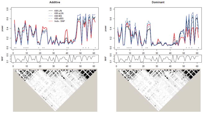
Top: Power to detect causal SNP for FGFR2 using additive (left) and dominant (right) genetic models under MED heritability due to SNP (max(h²)=1%). SNPs are ordered according to genomic location. Lines in gray and blue correspond to KM-based methods, whereas different line types and widths differentiate between types of kernels; the red solid line corresponds to the multiple testing adjusted individual-SNP based approach. The typed SNPs, indicated by an ‘x’ along the bottom of the plot, compose the SNP set. Middle: Corresponding MAF for SNPs plotted above. Bottom: Corresponding LD plot for SNPs plotted above (grayscale for squared correlation R²: white - R² = 0, black - R² = 1).

Figure 3 shows the analogous results for gene ASAH1. Note again that power is influenced by the MAF of the causal SNP. In particular, SNPs 1 and 28 in the top panel of Figure 3 have the lowest MAFs (0.083 and 0.058, respectively) causing them to have low power across all methods. The LD plots at the bottom indicate that the SNPs have much higher correlation as compared to FGFR2. To help see how power is affected by this correlation, the plots in Figure 4 show the same information as the top row of Figure 3, but with SNPs on the x-axis sorted by increasing median R² value. Here, median R² is defined as median squared correlation of the causal SNP with the SNPs in the SNP set. As this measure of correlation increases, so does the power of the kernel-based methods.

Figure 3.

Power to detect causal SNP for ASAH1 using additive (left) and dominant (right) genetic models under MED heritability due to SNP (max(h²)=1%). Legend is the same as Figure 2.

Figure 4.

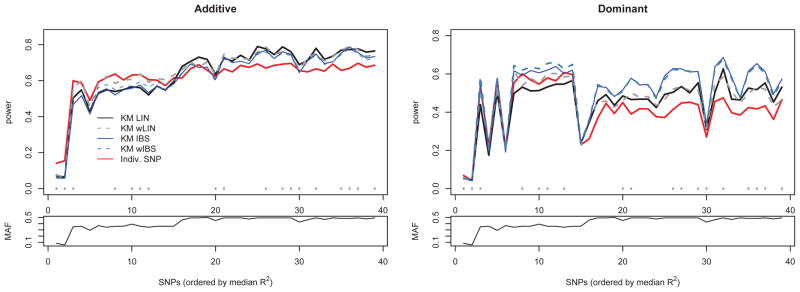
Top: Power to detect causal SNP for ASAH1 using additive (left) and dominant (right) genetic models under MED heritability due to SNP (max(h²)=1%). SNPs are ordered according to median R². Legend is the same as Figure 2. Bottom: Corresponding MAF for SNPs plotted above.

While the results in Figures 2, 3, and 4 depict the simulation involving the MED SNP heritability level (max(h²)=1%), the results are similar for both the LOW (max(h²)=0.5%) and HIGH (max(h²)=2%) SNP heritability scenarios, with the power curves shifting down and up, respectively. Focusing on only the kernel based methods in Figures 2–4, the linear and weighted linear kernels achieve the highest power when the data are generated under the linear additive genetic model, while the IBS and weighted IBS kernels achieve highest power when the SNP effects are generated under the dominant (nonlinear) model. Additionally, power for the weighted and unweighted versions of the same kernel type are similar, but there tends to be a slight gain in power for the weighted version when the causal SNP has low MAF.

Finally, we remark on the impact of including all HapMap SNPs (as opposed to just typed SNPs) in the SNP set to better understand the effect of the size (r) of the SNP set. Using all HapMap SNPs in the region, power can remain the same, increase, or decrease from that found using only ‘typed’ SNPs in the set (see Figure 4 in the Supporting Information). Indeed, the change in power depends on several factors, including whether the causal SNPs are genotyped, the level of LD between the causal SNPs and the typed SNPs, and the number of untyped SNPs that are null SNPs. For example, power for detecting untyped causal SNPs tends increase when all HapMap SNPs are used to define the SNP set, but the amount of improvement is much more drastic for FGFR2 than ASAH1. This is because the typed SNPs in ASAH1 already well-captured the nearby untyped SNPs, whereas the typed SNPs in FGFR2 did not. This observation in ASAH1 is consistent with the results found in Lin et al. [2011] based on including imputed SNPs, in addition to typed SNPs, in the SNP set. However, if the additional SNPs in the set are null SNPs with little to no correlation with the causal SNP, power of the kernel-based tests could decrease when using all HapMap SNPs in the set. Furthermore, the change in power for individual-SNP based analysis is also influenced by the (effective) number of additional SNPs, due to the adjusted p-value computation accounting for more multiple tests; i.e., gains in power by including causal SNPs could be offset by including too many additional SNPs in the set.

4.2 Influence of Ascertainment

Regarding the influence of ascertainment, the empirical size estimates for the kernel-based tests are reported in Table 2. As expected, with weak association of disease and secondary trait, the size estimates have negligible bias in type I error rate. While the distributions for the regression coefficients α under the null model were essentially the same, regardless of sampling mechanism, there were small differences in the null estimates of the variance components. Figure 5 displays the distribution of the variance component estimates under the null model for both non-random (solid histogram) and random selection (dashed histogram) of families. Under non-random ascertainment, ${\sigma }_b^2$ tends to be slightly underestimated while ${\sigma }_e^2$ tends to be slightly overestimated. In terms of power, the relative ordering of the curves under non-random ascertainment remained the same as under random family selection. In addition, the differences in power resulting from non-random ascertainment and random selection of families is generally small, as observed in the top portion of Figure 6. Interestingly, the largest differences (~0.15 in magnitude) occur at SNPs 3, 18 and 21, where there are few typed SNPs available in the set.

Table 2.

Empirical size based on candidate gene ASAH1 when sibship trios are ascertained according to disease status (at least one sibling must have disease); $v_{0b}={\sigma }_b^2{[{\sigma }_b^2+{\sigma }_e^2]}^{-1}=0.50$.

	Kernel
	LIN	wLIN	IBS	wIBS
Satterthwaite	0.049	0.050	0.053	0.054
Davies	0.049	0.051	0.053	0.053

Figure 5.

Distribution of Variance Component Estimates under the null hypothesis of no SNP Set effect: histograms with solid, black borders are for estimates computed using non-random selection of families (ascertained according to disease status), while the overlaid histograms in dashed-blue are for estimates computed using random selection of families. True parameter values are indicated by vertical red lines.

Figure 6.

Top: Difference in power to detect causal SNP for ASAH1 (additive genetic model under MED heritability due to SNP) between simulations where families were randomly selected and non-randomly selected based on at least one sibling have a disease. SNPs are ordered according to genomic location. Legend is similar to that in Figure 2, except that curves represent the subtraction of power using non-random (NR) family selection from power using random (R) family selection. Middle: Corresponding MAF for SNPs plotted above. Bottom: Corresponding LD plot for SNPs plotted above (grayscale for squared correlation R²: white - R² = 0, black - R² = 1).

4.3 SNP Sets along Chromosome 10

For the simulations involving SNPs sets based on different genes on chromosome 10, we ultimately computed 10000 p-values for significance under the null and alternative models for both the kernel machine and individual-SNP based multiple-testing corrected tests. To summarize these results, we computed empirical size across all 10000 simulations, as well as by binning the 10000 simulations into three groups based on SNP set size (r): r ≤ 10, 10 < r ≤ 20, and r > 20. The results in Table 3 reveal that the size estimates from the kernel-based test for theoretical size 0.05 remain accurate. We computed power after binning the 10000 simulations based on SNP set size (r), and then also by the median R² between the causal and typed SNPs. In particular, we split the simulations again into the three groups: r ≤ 10, 10 < r ≤ 20, and r > 20. We then further divided each of the three groups into subgroups by sorting the simulated SNP sets based on median R², and splitting the group into 50 evenly sized subgroups. Within each subgroup, we estimated the power as the proportion of p-values less than α = 0.05. For each of the groups, we plot lowess-smoothed power against median R² in Figure 7. A similar approach was used in Wu et al. [2010], where it was noted that the categorization by SNP set size (r) is needed because distantly located SNPs tend to be uncorrelated so that median R² tends to decrease with increasing r. As expected, power for both the kernel- and individual-SNP-based methods increases as heritability due to SNP (h²) increases. Also, under a variety of LD structures, we tend to see improved power for the kernel-based method over the individual-SNP based multiple testing method as the correlation, as measured by median R², increases, even when simulating under the additive, single-causal SNP model given in (10).

Table 3.

Empirical size by SNP set size for Chromosome 10 simulation, using the linear kernel for n = 300 sib trios under different polygenic effects. Size estimates computed using p-values from Davies method; Satterthwaite’s method yields qualitatively and quantitatively similar results.

SNP Set Size	# of Sets	v0b
		0.25	0.50	0.75
r ≤ 10	4244	0.050	0.055	0.050
10 < r ≤ 20	2831	0.047	0.057	0.052
r > 20	2925	0.046	0.054	0.049
All	10000	0.048	0.055	0.050

^* $v_{0b}={\sigma }_b^2{[{\sigma }_b^2+{\sigma }_e^2]}^{-1}$ is the heritability due to polygenic effects for within-family correlation.

Figure 7.

Power from Chromosome 10 simulation, plotted as a function of median R² for differing ranges of total number of SNPs in the SNP set (r). Different line types correspond to LOW, MED, and HIGH heritability due to SNP (h²).

5 Data Analysis

One long-term objective of the GENOA study is the elucidation of genetic susceptibility to atherosclerotic complications involving the heart. It is widely accepted that high levels of C-Reactive Protein (CRP), a heritable marker of chronic inflammation, are associated with increased risk of mortality and major diseases such as coronary heart disease [e.g., Dehghan et al., 2011]. At least two GWAS studies [Ridker et al., 2008; Dehghan et al., 2011] have implicated SNPs near the region of the genome encoding the leptin receptor (LEPR) as affecting levels of CRP, with both studies requiring a relatively large number of samples (>4000 and >66000 subjects, respectively) to identify SNPs reaching genome-wide significance at α = 5 × 10⁻⁸. We sought to replicate this finding in a much smaller dataset from the family-based GENOA study. Eligibility of families for the GENOA study requires that a sibship has two individuals diagnosed with essential hypertension before the age of 60 years; any normotensive siblings within the eligible sibships were also included. In particular, genotyped SNPs near and within the LEPR gene, as well as measures of CRP, are available for 881 subjects of European ancestry from 410 independent families.

Using both measured (Affymetrix 6.0) and imputed SNPs [MACH, Li et al., 2009], we examined the haplotypic block of SNPs that included the previously implicated ‘lead’ SNPs from Ridker et al. [2008] and Dehghan et al. [2011]. Figure 8 (left) shows the Haploview LD plot for the desired region using the CEU samples within HapMap. This block contains 106 common SNPs (15 were genotyped in the GENOA study and the rest were imputed) located near or within the LEPR gene (on 1p31) which will compose our SNP set. As the SNPs in the region are quite correlated (Figure 8), the multiple-SNP KM-based analysis has the potential to be more powerful than the individual-SNP based approach. As observed in Section 4.1, the additional correlation gained by including the imputed SNPs will likely be advantageous to the kernel-based analysis if the imputed SNPs are correlated with the unknown causal variant(s). We performed both SNP set tests, the KM SNP set test and the individual-SNP-based minimum p-value test adjusting for multiple comparisons, with response log(CRP) and covariates age, gender, body mass index, and smoking status. Note that after adjusting for these covariates, hypertension status and log(CRP) levels were not significantly associated (p = 0.161).

Figure 8.

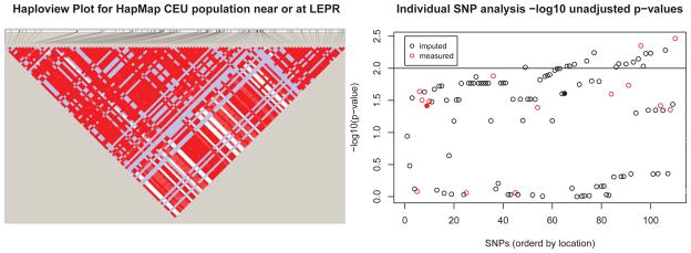
LD plot (standard D′/LOD color coding) using HapMap CEU population for the SNPs in the SNP set (left) and the individual-SNP analysis −log10 unadjusted p-values for the GENOA dataset, ordered by SNP location (right). The solid, filled-in circles, indicate the previously published ‘lead’ SNPs.

Individual-SNP analysis using lmekin revealed 17 SNPs with unadjusted p-values <0.01 (Figure 8, right; with previously implicated ‘lead’ SNPs depicted by solid, filled-in circles). Taking into account multiple testing for correlated SNPs using the method described in the simulations, the minimum adjusted [Conneely and Boehnke, 2007] individual-SNP based p-value was 0.039. For the KM SNP set analysis, we chose the weighted IBS kernel as there is a range of MAF values and the IBS kernel tends to perform well in both linear and more complex genetic models in simulation. The KM SNP set analysis p-value for the set using this choice of kernel was 0.010. For comparison, the KM SNP set p-values obtained using the linear, weighted linear, and IBS kernels were 0.013, 0.014, and 0.011, respectively. Indeed, regardless of the kernel function used, the KM-based analysis yields a lower p-value than that from the multiple testing-adjusted individual-SNP based analysis, as the KM test was able to borrow information across multiple correlated SNPs within the SNP set.

6 Discussion

We have proposed a kernel machine based framework for SNP set analysis for continuous outcomes when the subjects come from multiple different families. The underlying model can incorporate families of various sizes and relationships within the same association analysis. The proposed test is a score based-variance component test, which relies only on fitting the null linear mixed model (which needs only to be computed once for a GWAS dataset) to compute the test statistic. Notably the p-values are computed analytically, without the need for permutation, as we have shown that these values are accurate for even very small α levels. Furthermore, our simulations verify that when the causal SNP is correlated with multiple typed SNPs, the KM-based tests have improved power over the individual-SNP based analysis based on minimum adjusted p-values.

Like the SNP set based tests for independent subjects, the approach takes advantage of prior biological knowledge to group the SNPs into sets and each set is tested as an easily interpretable single entity. This not only has the potential to improve power by decreasing the number of tests in a genome-wide setting, but also by borrowing strength and information from correlated SNPs grouped together. Additionally, the KM approach allows for flexible modeling the SNP set effects on phenotype by specifying different kernel functions. The proposed methodology is valid irrespective of the selected kernel and SNP sets, but the power of the approach will be affected by the choice of kernel and choice of grouping. The best choice of kernel in terms of the most power improvement is an open question, but we have found that the (weighted) IBS kernel performs quite well in most simulated settings in that it loses little power when the effect of the SNP is linear, but can gain power when the effects of the SNPs are more complex.

Using the IBS kernel, our approach incorporates information on allele sharing among individuals within and between families to construct an appropriate test statistic of association. With pedigree data, we also possess information on alleles shared IBD within families. An open question then becomes whether we can use this IBD information to construct an association test similar to our existing IBS-based test. However, due to the fact that pairs of individuals from different families are unrelated and by definition share 0 alleles IBD, we believe a variance-component score test using an IBD kernel is not a test of association in a population of related subjects (since it ignores information from alleles shared across families) but rather is a test of linkage within families. To support this idea, we note that application of model (3) using a kernel matrix K derived from the proportion of alleles shared IBD at a gene will lead to the same variance-component model previously used for linkage analysis of quantitative traits [Amos, 1994; Almasy and Blangero, 1998].

The choice of SNP grouping will also influence power, as the amount of information available to borrow across SNPs depends on the SNPs present in the set. In particular, the KM based SNP set test improves power over the individual SNP based minimum p-value test when there is at least moderate LD among the SNPs in a SNP set, or in the presence of multiple causal variants within the set. If there are only a few causal SNPs (or few SNPs in LD with the causal SNP) in a set of predominantly null SNPs, power gains may not be realized. In the simulations and data analysis, we grouped SNPs based on either their proximity to a gene, or on the basis of LD structure in order to take advantage of the correlation of nearby SNPs. As previously mentioned, while we have the ability to model joint effects of multiple causal SNPs and epistatic effects, using the above strategies will only be able to identify these multiple SNP effects if they are located close enough to one another to be placed in the same SNP set. While it is not clear what the best strategy is for capturing the effects of multiple distantly-located SNPs, forming SNP sets based on gene pathways or networks can potentially help capture these effects.

The simulations and data analysis considered in this paper both focused on common variant SNP effects. However, the family-based KM approach can also easily be applied in sequencing association studies for rare variant effects. In these situations, it is often desirable to up-weight rare variants [e.g., Kryukov et al., 2007]. This can naturally be accommodated by appropriately specifying weights, w, in the kernel function. For example, if rarer variants (e.g., MAF ≤ 5%) are expected to be more likely to have larger effects, Wu et al. [2011] recommend setting 0 < α₁ ≤ 1 and α₂ ≥ 1 in $\sqrt{w_t}=\mathit{Beta}({\mathit{MAF}}_t,{\alpha }_1,{\alpha }_2)$ to up-weight rarer variants and down-weight common variants (e.g., α₁ = 1, α₂ = 25) for sequencing association studies. Such analyses could be beneficial in family-based data, for example, if members within the same family carry the same rare mutation while other families may carry different mutations within the same gene (SNP set).

The simulations also examined the influence of ascertainment on the KM test when the families were selected based on the presence of disease, but association between disease and continuous phenotype was weak. Under this scenario, our simulations confirmed that there is little to no inflation in type I error rate. These results are consistent with those in Monsees et al. [2009] regarding case-control ascertainment: when the association between secondary outcome and primary outcome (disease) is weak, ascertainment bias is negligible. In the context of case-control studies, Monsees et al. [2009] found in simulation that ascertainment bias is generally quite small except when both the genetic marker and secondary outcome are associated with disease. In this situation for family-based data, proper accounting for ascertainment (e.g., inverse probability weighting) would likely be needed and is an area for future research. In addition, our results are also in agreement with those in de Andrade and Amos [2000], who examined the impact of ascertainment bias on the testing of variance parameters in variance-component linkage analyses of quantitative traits. The authors found that the assessing major-gene effect using Wald and Likelihood Ratio tests in a variance-component model was not affected by ascertainment bias.

The proposed methods can be extended for more complicated models. For example, one can extend the proposed test to accommodate binary outcomes in family studies. An estimating equation based approach is currently being investigated to handle non-normal data, with results to be reported in a separate manuscript. Additionally, alternative random effects could be considered to model within-family (or generic within-group) correlation structures. A key advantage of the proposed methodology is that it allows for flexible modeling of the relationship between SNPs within a set and the outcome of interest. This will become an increasingly valuable feature as our understanding of the underlying biological processes, and hence our modeling abilities, improves.

Appendix

To show that Q under τ = 0 can be expressed as a mixture of chi-square distributions, note that P = V⁻¹ − V⁻¹X(X^TV⁻¹X)⁻¹X^T V⁻¹ for V evaluated under the null model can be expressed as P = V^−1/2MV^−1/2 where

$$\mathbf{M}=\mathbf{I}-{\mathbf{V}}^{-1/2}\mathbf{X}{({\mathbf{X}}^T{\mathbf{V}}^{-1}\mathbf{X})}^{-1}{\mathbf{X}}^T{\mathbf{V}}^{-1/2}$$

is an idempotent matrix. Thus

$$\begin{array}{l}\frac{1}{2}{\mathbf{y}}^T\mathbf{PKPy}=\frac{1}{2}{\mathbf{y}}^T{\mathbf{V}}^{-1/2}{\mathbf{MV}}^{-1/2}\mathbf{K}{\mathbf{V}}^{-1/2}{\mathbf{MV}}^{-1/2}\mathbf{y}\\ =\frac{1}{2}{\stackrel{\sim }{\mathbf{y}}}^T{\mathbf{MV}}^{-1/2}\mathbf{K}{\mathbf{V}}^{-1/2}\mathbf{M}\stackrel{\sim }{\mathbf{y}}\end{array}$$

where MV^−1/2y = Mỹ and ỹ ~ N(0,I). Let λ₁ ≥ … ≥ λ_q > 0 be the q ≤ n ordered non-zero eigenvalues of $\overline{\mathbf{K}}=\frac{1}{2}{\mathbf{MV}}^{-1/2}\mathbf{K}{\mathbf{V}}^{-1/2}\mathbf{M}$ and Λ= diag(λ_i i = 1,…,q). Let E be the q × n matrix of eigenvectors corresponding to λ_i such that EE^T = I. Then,

$$\frac{1}{2}{\mathbf{y}}^T\mathbf{PKPy}={\stackrel{\sim }{\mathbf{y}}}^T{\mathbf{E}}^T\mathrm{\Lambda }\mathbf{E}\stackrel{\sim }{\mathbf{y}}=\sum {\lambda }_i{z}_i^2$$

where z = (z₁,…,z_q)^T = Eỹ and z_i ~ iidN(0,1). Thus, $\frac{1}{2}{\mathbf{y}}^T\mathbf{PKPy}$ is a mixture of chi-square distributions, each with one degree of freedom.

Specifically for the Satterthwaite approximation with $\mathit{\vartheta }=({\sigma }_b^2,{\sigma }_e^2)$, we calculate κ̂ = /2μ̃ and ν̂ = 2μ̃²/ where ${\stackrel{\sim }{\mathcal{I}}}_{\tau \tau }={\mathcal{I}}_{\tau \tau }-{\mathcal{I}}_{\tau \mathit{\vartheta }}{\mathcal{I}}_{\mathit{\vartheta }\mathit{\vartheta }}^{-1}{\mathcal{I}}_{\tau \mathit{\vartheta }}^T$ with

$${\mathcal{I}}_{\tau {\mathit{\vartheta }}_j}=\frac{1}{2}tr\left(\mathbf{PKP}\frac{\partial \mathbf{V}}{\partial {\mathit{\vartheta }}_j}\right)\text{and}{\mathcal{I}}_{{\mathit{\vartheta }}_j{\mathit{\vartheta }}_k}=\frac{1}{2}tr\left(\mathbf{P}\frac{\partial \mathbf{V}}{\partial {\mathit{\vartheta }}_j}\mathbf{P}\frac{\partial V}{\partial {\mathit{\vartheta }}_k}\right),$$

and all terms are evaluated at ϕ̂, which is the ML or REML estimate calculated under the null model (6). This leads to the test statistic Q(ϕ̂)/κ̂ with approximate null distribution ${\chi }_{\widehat{\nu }}^2$.

In the implementation of Davies method, we use the eigenvalues of K̄, where the null estimates of ${\sigma }_b^2$ and ${\sigma }_e^2$ are used to calculate V, to compute the p-values for test statistic Q(ϕ̂), for ϕ̂ again representing the ML or REML estimator under the null model. Note that with a small number of covariates, both the ML and REML versions of the statistics perform quite similarly when the sample size is decent.

References

- Abecasis GR, Cardon LR, Cookson WO. A general test of association for quantitative traits in nuclear families. Am J Hum Genet. 2000;66:279–292. doi: 10.1086/302698. [DOI] [PMC free article] [PubMed] [Google Scholar]
- Almasy L, Blangero J. Multipoint quantitative-trait linkage analysis in general pedigrees. Am J Hum Genet. 1998;62:1198–1211. doi: 10.1086/301844. [DOI] [PMC free article] [PubMed] [Google Scholar]
- Altschuler D, Brooks L, Chakravarti A, Collins F, Daly M, Donnelly P. International hapmap consortium. a haplotype map of the human genome. Nature. 2005;437:1299–1320. doi: 10.1038/nature04226. [DOI] [PMC free article] [PubMed] [Google Scholar]
- Amos CI. Robust variance-components approach for assessing genetic linkage in pedigrees. Am J Hum Genet. 1994;54:535–543. [PMC free article] [PubMed] [Google Scholar]
- Atkinson B, Therneau T. R package version 1.1.0-23. 2009. kinship: mixed-effects Cox models, sparse matrices, and modeling data from large pedigrees. [Google Scholar]
- Conneely KN, Boehnke M. So Many Correlated Tests, So Little Time! Rapid Adjustment of P Values for Multiple Correlated Tests. Am J Hum Genet. 2007:81. doi: 10.1086/522036. [DOI] [PMC free article] [PubMed] [Google Scholar]
- Daniels PR, Kardia SL, Hanis CL, Brown CA, Hutchinson R, et al. Familial aggregation of hypertension treatment and control in the Genetic Epidemiology Network of Arteriopathy (GENOA) study. Am J Med. 2004;116:676–681. doi: 10.1016/j.amjmed.2003.12.032. [DOI] [PubMed] [Google Scholar]
- Davies R. Algorithm as 155: The distribution of a linear combination of chi-2 random variables. Journal of the Royal Statistical Society: Series C (Applied Statistics) 1980;29:323–333. [Google Scholar]
- de Andrade M, Amos CI. Ascertainment issues in variance components models. Genet Epidemiol. 2000;19:333–344. doi: 10.1002/1098-2272(200012)19:4<333::AID-GEPI5>3.0.CO;2-#. [DOI] [PubMed] [Google Scholar]
- Dehghan A, Dupuis J, Barbalic M, Bis JC, Eiriksdottir G, et al. 80 000 subjects identifies multiple loci for C-reactive protein levels. Circulation. 2011;123:731–738. doi: 10.1161/CIRCULATIONAHA.110.948570. [DOI] [PMC free article] [PubMed] [Google Scholar]
- FBPP Investigators. Multi-center genetic study of hypertension: The Family Blood Pressure Program (FBPP) Hypertension. 2002;39:3–9. doi: 10.1161/hy1201.100415. [DOI] [PubMed] [Google Scholar]
- Fields LE, Burt VL, Cutler JA, Hughes J, Roccella EJ, Sorlie P. The burden of adult hypertension in the United States 1999 to 2000: a rising tide. Hypertension. 2004;44:398–404. doi: 10.1161/01.HYP.0000142248.54761.56. [DOI] [PubMed] [Google Scholar]
- Gao X, Starmer J, Martin ER. A multiple testing correction method for genetic association studies using correlated single nucleotide polymorphisms. Genet Epidemiol. 2008;32:361–369. doi: 10.1002/gepi.20310. [DOI] [PubMed] [Google Scholar]
- Gianola D, van Kaam JB. Reproducing kernel hilbert spaces regression methods for genomic assisted prediction of quantitative traits. Genetics. 2008;178:2289–2303. doi: 10.1534/genetics.107.084285. [DOI] [PMC free article] [PubMed] [Google Scholar]
- Han F, Pan W. Powerful multi-marker association tests: unifying genomic distance-based regression and logistic regression. Genet Epidemiol. 2010;34:680–688. doi: 10.1002/gepi.20529. [DOI] [PMC free article] [PubMed] [Google Scholar]
- Jacquard A. The genetic structure of populations. New York: Springer-Verlag; 1974. [Google Scholar]
- Kimeldorf G, Wahba G. Some results on Tchebycheffian spline functions. Journal of Mathematical Analysis and Applications. 1970;33:82–95. [Google Scholar]
- Kryukov GV, Pennacchio LA, Sunyaev SR. Most rare missense alleles are deleterious in humans: implications for complex disease and association studies. Am J Hum Genet. 2007;80:727–739. doi: 10.1086/513473. [DOI] [PMC free article] [PubMed] [Google Scholar]
- Kumar P, Henikoff S, Ng PC. Predicting the effects of coding non-synonymous variants on protein function using the SIFT algorithm. Nature Protocols. 2009;4:1073–1081. doi: 10.1038/nprot.2009.86. [DOI] [PubMed] [Google Scholar]
- Kwee LC, Liu D, Lin X, Ghosh D, Epstein MP. A powerful and flexible multilocus association test for quantitative traits. Am J Hum Genet. 2008;82:386–397. doi: 10.1016/j.ajhg.2007.10.010. [DOI] [PMC free article] [PubMed] [Google Scholar]
- Li Y, Willer C, Sanna S, Abecasis G. Genotype imputation. Annual Review of Genomics and Human Genetics. 2009;10:387–406. doi: 10.1146/annurev.genom.9.081307.164242. [DOI] [PMC free article] [PubMed] [Google Scholar]
- Lin WY, Schaid DJ. Power comparisons between similarity-based multilocus association methods, logistic regression, and score tests for haplotypes. Genet Epidemiol. 2009;33:183–197. doi: 10.1002/gepi.20364. [DOI] [PMC free article] [PubMed] [Google Scholar]
- Lin X. Variance component testing in generalized linear models with random effects. Biometrika. 1997;84:309–326. [Google Scholar]
- Lin X, Cai T, Wu MC, Zhou Q, Liu G, Christiani DC, Lin X. Kernel machine SNP-set analysis for censored survival outcomes in genome-wide association studies. Genet Epidemiol. 2011;35:620–631. doi: 10.1002/gepi.20610. [DOI] [PMC free article] [PubMed] [Google Scholar]
- Liu D, Ghosh D, Lin X. Estimation and Testing for the Effect of a Genetic Pathway on a Disease Outcome using Logistic Kernel Machine Regression via Logistic Mixed Models. BMC Bioinformatics. 2008:9. doi: 10.1186/1471-2105-9-292. [DOI] [PMC free article] [PubMed] [Google Scholar]
- Liu D, Lin X, Ghosh D. Semiparametric Regression of Multi-Dimensional Genetic Pathway Data: Least Square Kernel Machines and Linear Mixed Models. Biometrics. 2007;63:1079–1088. doi: 10.1111/j.1541-0420.2007.00799.x. [DOI] [PMC free article] [PubMed] [Google Scholar]
- Liu JZ, McRae AF, Nyholt DR, Medland SE, Wray NR, Brown KM, Hayward NK, Montgomery GW, Visscher PM, Martin NG, Macgregor S, Mann GJ, Kefford RF, Hopper JL, Aitken JF, Giles GG, Armstrong BK. A versatile gene-based test for genome-wide association studies. Am J Hum Genet. 2010;87:139–145. doi: 10.1016/j.ajhg.2010.06.009. [DOI] [PMC free article] [PubMed] [Google Scholar]
- Manolio TA, Collins FS, Cox NJ, Goldstein DB, Hindorff LA, et al. Finding the missing heritability of complex diseases. Nature. 2009;461:747–753. doi: 10.1038/nature08494. [DOI] [PMC free article] [PubMed] [Google Scholar]
- Monsees GM, Tamimi RM, Kraft P. Genome-wide association scans for secondary traits using case-control samples. Genet Epidemiol. 2009;33:717–728. doi: 10.1002/gepi.20424. [DOI] [PMC free article] [PubMed] [Google Scholar]
- Moskvina V, Schmidt KM. On multiple-testing correction in genome-wide association studies. Genet Epidemiol. 2008;32:567–573. doi: 10.1002/gepi.20331. [DOI] [PubMed] [Google Scholar]
- Mukhopadhyay I, Feingold E, Weeks DE, Thalamuthu A. Association tests using kernel-based measures of multi-locus genotype similarity between individuals. Genet Epidemiol. 2010;34:213–221. doi: 10.1002/gepi.20451. [DOI] [PMC free article] [PubMed] [Google Scholar]
- Pan W. Asymptotic tests of association with multiple SNPs in linkage disequilibrium. Genet Epidemiol. 2009;33:497–507. doi: 10.1002/gepi.20402. [DOI] [PMC free article] [PubMed] [Google Scholar]
- Price AL, Patterson NJ, Plenge RM, Weinblatt ME, Shadick NA, Reich D. Principal components analysis corrects for stratification in genome-wide association studies. Nature Genetics. 2006;38:904–909. doi: 10.1038/ng1847. [DOI] [PubMed] [Google Scholar]
- Rakovski CS, Xu X, Lazarus R, Blacker D, Laird NM. A new multimarker test for family-based association studies. Genet Epidemiol. 2007;31:9–17. doi: 10.1002/gepi.20186. [DOI] [PubMed] [Google Scholar]
- Ramensky V, Bork P, Sunyaev S. Human non-synonymous SNPs: server and survey. Nucleic Acids Research. 2002;30:3894–3900. doi: 10.1093/nar/gkf493. [DOI] [PMC free article] [PubMed] [Google Scholar]
- Ridker PM, Pare G, Parker A, Zee RY, Danik JS, et al. Loci related to metabolic-syndrome pathways including LEPR, HNF1A, IL6R, and GCKR associate with plasma C-reactive protein: the Women’s Genome Health Study. Am J Hum Genet. 2008;82:1185–1192. doi: 10.1016/j.ajhg.2008.03.015. [DOI] [PMC free article] [PubMed] [Google Scholar]
- Schaid DJ, Rowland CM, Tines DE, Jacobson RM, Poland GA. Score tests for association between traits and haplotypes when linkage phase is ambiguous. Am J Hum Genet. 2002;70:425–434. doi: 10.1086/338688. [DOI] [PMC free article] [PubMed] [Google Scholar]
- Schölkopf B, Herbrich R, Smola AJ. A generalized representer theorem. Proceedings of the 14th Annual Conference on Computational Learning Theory and and 5th European Conference on Computational Learning Theory; London, UK: Springer-Verlag; 2001. pp. 416–426. COLT ’01/EuroCOLT ’01. [Google Scholar]
- Spencer C, Su Z, Donnelly P, Marchini J. Designing genome-wide association studies: sample size, power, imputation, and the choice of genotyping chip. PLoS Genet. 2009:5. doi: 10.1371/journal.pgen.1000477. [DOI] [PMC free article] [PubMed] [Google Scholar]
- Tzeng JY, Zhang D, Chang SM, Thomas D, Davidian M. Gene-trait similarity regression for multimarker-based association analysis. Biometrics. 2009;65:822–832. doi: 10.1111/j.1541-0420.2008.01176.x. [DOI] [PMC free article] [PubMed] [Google Scholar]
- Tzeng JY, Zhang D, Pongpanich M, Smith C, McCarthy MI, et al. Studying gene and gene-environment effects of uncommon and common variants on continuous traits: a marker-set approach using gene-trait similarity regression. Am J Hum Genet. 2011;89:277–288. doi: 10.1016/j.ajhg.2011.07.007. [DOI] [PMC free article] [PubMed] [Google Scholar]
- Wessel J, Schork NJ. Generalized genomic distance-based regression methodology for multilocus association analysis. Am J Hum Genet. 2006;79:792–806. doi: 10.1086/508346. [DOI] [PMC free article] [PubMed] [Google Scholar]
- Wu MC, Kraft P, Epstein MP, Taylor DM, Chanock SJ, Hunter DJ, Lin X. Powerful SNP-set analysis for case-control genome-wide association studies. Am J Hum Genet. 2010;86:929–942. doi: 10.1016/j.ajhg.2010.05.002. [DOI] [PMC free article] [PubMed] [Google Scholar]
- Wu MC, Lee S, Cai T, Li Y, Boehnke M, Lin X. Rare variant association testing for sequencing data using the sequence kernel association test (skat) 2011. submitted. [DOI] [PMC free article] [PubMed] [Google Scholar]
- Zhang D, Lin X. Hypothesis testing in semiparametric additive mixed models. Biostatistics. 2003;4:57–74. doi: 10.1093/biostatistics/4.1.57. [DOI] [PubMed] [Google Scholar]
Associated Data
This section collects any data citations, data availability statements, or supplementary materials included in this article.